Project report
Analysis of the evolution of the climate parameters, especially
precipitations and temperatures, in the province of Binh Thuan in
Southern Vietnam based on IPCC models
S´ebastien DOUTRELOUP · Xavier FETTWEIS · Pierre OZER
10thAugust 2010
1 Introduction
This research is implied into the BELSPO / Vietnamese de-sertification project and The aim of this work is to anal-yse the future evolution of the temperatures and precipita-tions in the region of Binh Thuan. This region is situated in the southern Vietnam. This study is realized within the framework of the project entitled “Impact of global climate change and desertification on the environment and society in Southern Central Vietnam - Case study in Binh Thuan Province ”.
The climate of this region is caracterised by a monsoon [NIEUWOLT S., 1981]. There are two distinct periods ; a
S. Doutreloup
Department of Geography, Laboratory of Climatology University of Li`ege
All´ee du 6 Aout, 2, 4000 Li`ege, Belgium Tel.: +32-43-665354
Fax: +32-43-665722
E-mail: [email protected] X. Fettweis
Department of Geography, Laboratory of Climatology, University of Li`ege, Belgium E-mail: [email protected]
P. Ozer
Department of Sciences and Environment Management, University of Li`ege, Belgium E-mail: [email protected]
Fig. 1 Vietnam Topography with the interested region in a black rect-angle. Sources: http://fr.wikipedia.org/wiki/Viˆet Nam
dry period and a wet period. The dry period begins approx-imatively in November through April and the wet period from May through October. The wet season is caracterised by two maximum of precipitations. The first one is in May-June and the second one is in September-October. These maximum of precipitations are due to the round-trip of the monsoon. The first maximum occurs when the Inter-Tropical Convergence Zone (ITCZ) goes to the North. During this
2
passage, the air mass are satured in humidity thanks to all Indonesian water mass. And the second maximum occurs when the ITCZ goes to the South. During this passage, the air mass is also satured in humidity thanks to the South China Sea. The evolution of temperature is relatively con-stant through the year. The monthly mean temperatures os-cillate between 25oC and 30oC.
To analyse the future projections of the climate param-eters, we base our researchs on the the ECMWF reanalysis model, NCEP-NCAR reanalysis model and all the models proposed by the IPCC1.
2 Methodology
The final goal is to predict the trend of temperature and pre-cipitation in Southern Vietnam in the 21st century. For this
we use the future projections models selected by the IPCC. In a first time, we test the ability of each model to simulate the present climate (the period is 1970-1999) in Southern Vietnam, then we select the best models. In a second time, we use the future projections of these best models to obtain a trend of temperature and precipitation.
At the beginning, we have 24 differents models. Of course, all are not suitable to analyse the future projections. So, the first step is to sort them and keep some models which best simulate the present climate. For this aim, we compare the IPCC models with the ECMWF and NCAR Reanalysis.
We sort the models two times : The first sorting is to eliminate the worst models and obtain about the half of the total number of models and the second sorting is to keep the best models and obtain some models from which we use the projections of future climatic parameters and their evo-lutions.
1 Intergovernmental Panel on Climate Change: http://www.ipcc.ch/
At the first sorting, we use the daily data of the IPCC models, the ECMWF and NCAR Reanalysis during the pe-riod 1970-1999. For each IPCC models, we calculate the monthly mean of temperature at 2m and the monthly sum of precipitations. We also calculate for the reanalysis models the monthly standard error (σ ) for temperatures and precip-itations. Then we plot these data on a climograph2with the data of the IPCC models and we superimpose ±2σ of each reanalysis model.
The method to eliminate the worst IPCC models is based on 2 criteria :
– The curves of temperature and precipitations must re-spect the best the behaviour of the curves of reanalysis models. Especially, the curves of temperature and pre-cipitations must respect the best the different dry and wet periods.
– The curves of temperature and precipitations must be in-cluded as best as possible into the range of ±2σ .
At the second sorting, we use the selected models of the first sorting and we plot the temperatures and precipitations curves on two separate graphs which we add the curves of the maximum ±1σ of reanalysis models on a same time step. This sorting consists to keep the models which the curve is included or very near into the range determined by the ±1σ limits of the model. Thus we keep only the models which represent the best the reality given by the reanalysis.
After these two sortings, we can consider that all se-lected models represent the best the reality given by the reanalysis models and thus the models which represent the best the future. In that way, we can use these selected
mod-2 A climograph is a dual-purpose graph, it shows, on a same graph
and on the same period, the temperatures and the precipitations. The convention for the Y-axis is that precipitation represents two times the temperature.
3
els to project the trends of temperatures and precipitations in the future.
The analysis of the future trend is based on three steps : The first is the analyse of the basic climate statistics, the second is the analyse of the climographs and the third is the analyse of the beginning and end of the wet season :
– The first analysis consists of evaluate the future trend of climate parameters. The parameters is the annual mean temperature, annual amount of precipitation, standard-deviation of temperature and precipitation, maximum and minimum of temperature and precipitation, some inter-esting percentiles.
– The second analysis consists to create the climographs. Thanks to this climographs, we can evaluate the general behaviour of the climate in the studied region, the begin-ning and end of the wet season, and the trend of the two summit of precipitations during the year.
– This third analysis consists to calculate the beginning and the end of the wet season to predict either an expan-sion or a diminution of the duration of this wet season. With all these elements, we can concluded the future projection of the climate parameters in the province of Binh Thuan in Southern Vietnam.
3 Data
In this section, we present all the data used in this work : How do this data are constructed ? Where can we find it ? Advantage and disadvantage of using these data.
3.1 ECMWF & NCEP-NCAR Reanalysis
The reanalysis models in general are global models which calculate the past climate with a forcing of the meteorolog-ical observations including radiosondes, balloons, aircraft,
buoyes, satellites, scatterometers. We can consider the re-analysis as the best representations of the past climates.
The ECMWF reanalysis3is one of the reanalysis models used in climatology over the period from September 1957 through August 2002. In this task, we work only with the period from January 1970 through December 1999.
The NCEP-NCAR Reanalysis-14is one other reanalysis
models used in climatology over the period from January 1948 through present. In this task, we work only with the period from January 1970 through December 1999.
The advantage of using this kind of data is that the entire world is covered by at least one set of meteorological data. The disadvantage is that data over one region are interpo-lated compared with the real observation data in a meteoro-logical station. The interpolation is proportionnal with the spatial resolution of the model (we can see this resolution in the third column of the table 1).
A second advantage can be found in the nature of these data. Indeed, these one are calculated by a model. This fact implies that we compare two models among them and not local observations with a global model. The local observa-tions representent the climate of one site and is very difficult to apply to an entire region because the site have a lot of caracteristics which does not are not similar to the entire re-gion.
3.2 Models selected by the IPCC
The IPCC [IPCC AR4-WGI 2007] have selected 24 models in his last report AR4, as we can see in the Table 1. These models are forced by none observational data. All of these models have initial conditions, which are create randomly
3 ECWMF : European Center for Medium-range Weather Forecast
http://www.ecmwf.int/
4 NCEP-NCAR : National Centers for
Environmen-tal Prediction - National Center for Atmospheric Research http://www.cpc.ncep.noaa.gov/
4
and the models run from these initial conditions till obtain the equilibrium conditions.
According to their internal configurations, the models are different. Thus, some models are not consistent with the real climate, thus we must choose the models which repre-sent the better the reality.
All models have a different spatial resolution, as you can see in the third column of the Table 1. Some models have a relatively precise spatial resolution like the INGV model with 1.1◦ latitude and 1.1◦ longitude and whereas some models have a coarse spatial resolution like the GISS– EH model with 5.0◦latitude and 4.0◦ longitude. This fact imply that the interpolation of data over one region is bigger when the spatial resolution is coarse.
However we do not use all of these models because all data required in this work are sometimes not available. The models which can not be use are : BCCR, INMCM, HADCM3, and HADGEM1.
The IPCC models have different periods. Firstly, the IPCC models have a scenario called 20C3M which calculate the past climate over the period from the year 1961 through the year 2000. We use this scenario over the period from 1970 through 1999 in the two sortings to compare with reanalysis models.
Secondly, the IPCC models have differents periods in the future and also different scenarios. In this work, we use the period from the year 2046 through the year 2065 and the period from the year 2081 through the year 2100. In this work, we also use three scenarios : the scenario A1B, the scenario A2 and the scenario B1.
The A1B scenario [IPCC AR4-WGI 2007] is of a more integrated world. The A1B scenario is characterized by: a rapid economic growth, a global population that reaches 9 billion in 2050 and then gradually declines, the quick spread of new and efficient technologies, a convergent world -
in-Table 1 Models and reanalyses used in this study with their short name and spatial resolution. The AOGCMs short names are based on the work of [LELOUP et al. 2007]. Data source: the World Climate Research Programme’s (WCRP’s) Coupled Model Intercomparison Project phase 3 (CMIP3) multi–model dataset available at http://www– pcmdi.llnl.gov/.
Data name Short name Spatial resolution BCCR–BCM2.0 BCCR 2.8◦× 2.8◦ CCCMA–CGCM3.1(T47) CCCMA–T47 3.7◦× 3.7◦ CCCMA–CGCM3.1(T63) CCCMA–T63 2.8◦× 2.8◦ CNRM–CM3 CNRM 2.8◦× 2.8◦ CSIRO–Mk3.0 CSIRO–0 1.9◦× 1.9◦ CSIRO–Mk3.5 CSIRO–5 1.9◦× 1.9◦ GFDL–CM2.0 GFDL–0 2.6◦× 2.0◦ GFDL–CM2.1 GFDL–1 2.6◦× 2.0◦ GISS–AOM GISS–AOM 4.0◦× 3.0◦ GISS–EH GISS–EH 5.0◦× 4.0◦ GISS–ER GISS–ER 5.0◦× 4.0◦ IAP–FGOALS–g1.0 IAP 2.8◦× 2.8◦ INGV–SXG INGV 1.1◦× 1.1◦ INM–CM3.0 INMCM 5.0◦× 4.0◦ IPSL–CM4 IPSL 3.8◦× 2.5◦
MIROC3.2 (hires) MIROC–HR 1.1◦× 1.1◦
MIROC3.2 (medres) MIROC–MR 2.8◦× 2.8◦ MIUBECHO-G MIUB 3.7◦× 3.7◦ ECHAM5/MPI–OM MPI 1.9◦× 1.9◦ MRI–CGCM2.3.2 MRI 2.8◦× 2.8◦ NCAR–CCSM3 CCSM3 1.4◦× 1.4◦ NCAR–PCM1 PCM1 2.8◦× 2.8◦ UKMO–HadCM3 HADCM3 3.8◦× 2.5◦ UKMO–HadGEM1 HADGEM1 1.9◦× 1.2◦
ECMWF 40 Year Reanalysis ERA–40 1.1◦× 1.1◦
NCEP/NCAR Reanalysis 1 NCEP1 2.5◦× 2.5◦
come and way of life converge between regions. Extensive social and cultural interactions worldwide and a balanced emphasis on all energy sources.
The A2 scenario [IPCC AR4-WGI 2007] is of a more divided world. The A2 scenario is characterized by: a world of independently operating, self-reliant nations, a
continu-5
ously increasing population, a regionally oriented economic development, a slower and more fragmented technological changes and improvements to per capita income.
The B2 scenario [IPCC AR4-WGI 2007] are of a world more divided, but more ecologically friendly. The B2 sce-nario are characterized by: a continuously increasing popu-lation, but at a slower rate than in A2, an emphasis on local rather than global solutions to economic, social and envi-ronmental stability, an intermediate levels of economic de-velopment, a less rapid and more fragmented technological change than in A1 and B1.
4 Results of the first sorting
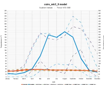
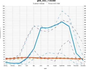
This first step consists to create the climograph of the re-analysis models. The X-axis represents the twelve months of the year, the left Y-axis represents the temperature in Cel-sius degrees and the right Y-axis represents the precipita-tions in millimeters. The values on the scale of the right Y-axis represents the double of the values on the left Y-Y-axis. The climograph of ECMWF can be see in the Fig.2 and the climograph of NCEP-NCAR in the Fig.3. Then we construct the same climograph with the IPCC models but we add the curves of ±2σ of the temperature and precipitations.
We analyse each climograph one by one to eliminate those which not respect the 2 criteria defined in the section 2. Here is the discussion of each models5:
– CCCMA-T47 : This model respects all the criteria. We accept it.
– CCCMA-T63 : This model is pretty good however the summit of precipitations of the late summer are a little too high. We do not accept it.
– CNRM : The dry season of this model is too short and the range of temperature is not respected. We do not ac-cept it.
5 We use the short name in the Table 1 to identify the model
Fig. 2 Climograph of the ECMWF reanalysis model with the error bars of ±2σ . The blue curve represents the precipitations and the red one the temperatures.
Fig. 3 Climograph of the NCEP-NCAR reanalysis model with the error bars of ±2σ . The blue curve represents the precipitations and the red one the temperatures.
– CSIRO-0 : This model have a wet season too high and exceeds the range defined by the ±2σ of the reanalysis model. We do not accept it.
– CSIRO-5 : This model have a wet season too high and exceeds the range defined by the ±2σ of the reanalysis model. The temperature curve is not include in the range defined by the ±2σ of the reanalysis model. We do not accept it.
6
– GFDL-0 : This model have a wet season too high and exceeds the range defined by the ±2σ of the reanalysis model. We do not accept it.
– GFDL-1 : This model have a wet season too high and exceeds the range defined by the ±2σ of the reanalysis model. We do not accept it.
– GISS-AOM : This model does not respect the behaviour of the curves of reanalysis. It does not distinguish the wet and dry season. We do not accept it.
– GISS-EH : This model have a dry season which have an exceed of precipitations. We do not accept it.
– GISS-ER : This model does not respect the behaviour of the curves of reanalysis. We do not accept it.
– IAP : This model does not respect the behaviour of the curves of reanalysis and the dry season is too long. We do not accept it.
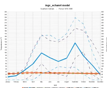
– INGV : This model respects all the criteria. We accept it.
– IPSL : This model respects all the criteria. We accept it. – MIROC-HR : This model have a wet season too high and exceeds the range defined by the ±2σ of the reanal-ysis model. We do not accept it.
– MIROC-MR : This model does not respect the behaviour of the curves of reanalysis and it have a dry season with a too high sum of precipitations. We do not accept it. – MIUB : This model have a wet season too long and
con-sequently a dry season too short. We do not accept it. – MPI : This model does not respect the behaviour of the
curves of reanalysis. It does not have a summit of pre-cipitations in the late summmer, and this part of the year have less precipitations than the spring summit of pre-cipitations. We do not accept it.
– MRI : This model have his first summit of precipitations which exceeds the range defined by the ±2σ of the re-analysis model. We do not accept it.
Fig. 4 Climograph of the CCCMA-T47 model with the reanalysis models error curve of ±2σ . The continuous blue curve represents the precipitations and the continuous red one the temperatures. The discontinuous blue curves represent the ±2σ of precipitations in the ECMWF reanalysis model and the discontinuous violet curves repre-sent the ±2σ of precipitations in the NCEP-NCAR reanalysis model. The discontinuous red curves represent the ±2σ of temperatures in the ECMWF reanalysis model and the discontinuous green curves repre-sent the ±2σ of temperatures in the NCEP-NCAR reanalysis model.
– CCSM3 : This model have a dry season too long and consequently a wet season too short. This model have also only one summit of precipitations in the late sum-mer and none in the spring. We do not accept it. – PCM1 : This model have his first summit of
precipita-tions which exceeds the range defined by the ±2σ of the reanalysis model. We do not accept it.
In conclusion, only 3 models respect the criteria defined in the section 2. : CCCMA-T47, INGV and the IPSL. We use these one in the second sorting.
7
Fig. 5 Same legend that the Fig.4 but with the CCCMA-T63 model
Fig. 6 Same legend that the Fig.4 but with the CNRM model
Fig. 7 Same legend that the Fig.4 but with the CSIRO-0 model
8
Fig. 9 Same legend that the Fig.4 but with the GFDL-0 model
Fig. 10 Same legend that the Fig.4 but with the GFDL-1 model
Fig. 11 Same legend that the Fig.4 but with the GFDL-AOM model
9
Fig. 13 Same legend that the Fig.4 but with the GFDL-ER model
Fig. 14 Same legend that the Fig.4 but with the IAP model
Fig. 15 Same legend that the Fig.4 but with the INGV model
10
Fig. 17 Same legend that the Fig.4 but with the MIROC-HR model
Fig. 18 Same legend that the Fig.4 but with the MIROC-MR model
Fig. 19 Same legend that the Fig.4 but with the MIUB model
11
Fig. 21 Same legend that the Fig.4 but with the MRI model
Fig. 22 Same legend that the Fig.4 but with the CCSM3 model
12
5 Results of the second sorting
This second sorting consists to eliminate the models which the curve is not include into the range determined by the ±1σ of the reanalysis models. The comparison of the se-lected models between the precipitation year curve of each models and the maximum of ±1σ between each reanalysis model is in the Fig.24. The comparison of the selected mod-els between the temperature year curve of each modmod-els and the maximum of ±1σ between each reanalysis model is in the Fig.25.
Fig. 24 Comparison of the precipitations of the selected models com-pared with the maximum standard error of the reanalysis models. The range determined by the maximum of ±1σ of each reanalysis mod-els is in black continuous lines. The CCCMA-T47 model is in yellow squarred line, the INGV model is in orange diamonded line and the IPSL model is in red triangulated line.
Globally, we can consider that all models are include into the range determined by the maximum of ±1σ of each reanalysis models. Thus we keep all the models selected by the first sorting. However, it is important to moderate the IPSL model. Indeed, this model has a summit of precipi-tations in the late summer which exceed the ±1σ of the reanalysis models. We keep it because elsewhere the
be-Fig. 25 Comparison of the temperature of the selected models com-pared with the maximum standard error of the reanalysis models. The range determined by the maximum of ±1σ of each reanalysis mod-els is in black continuous lines. The CCCMA-T47 model is in yellow squarred line, the INGV model is in orange diamonded line and the IPSL model is in red triangulated line.
haviour of the curve is into the range. The difference is that when we will analyse the future projection, we will pay at-tention to the fact that this model overestimates the late sum-mer summit of precipitations. We can do the same reflex-ion for the INGV model. Between February and March, this model slightly exceeds the range of precipitation. The tem-perature curve of IPSL model overestimates the temtem-perature range defined by the reanalysis model. This overestimation is approximatively of 14% compared to the mean of the re-analysis models. We will pay attention when we will analyse the future projections.
In conclusion, this second sorting is just a verification of the exactitude of the selected models of the first sorting. No models is excluded at this stage but the IPSL model must be watch.
13
6 Analysis of the future projections
We are sure that the three selected models represent the best the past climate. This task consists to obtain the future evo-lution of the climate parameters from these three selected models. For this aim, we analyse some basic statistics, the climographs and the beginning and end of the wet season for each model, each future periods and each scenario. How-ever, the INGV model does not have a simulation for the B1 scenario.
BASIC STATISTICAL ANALYSIS
In this part, we describe the future evolution of the ba-sic statistics : The mean of temperature, the standard error of both variables, the annual amount of precipitations, the maximum/minimum temperature and the maximum precip-itations found in the studied period, some interesting per-centiles and the persistance of 2 mm of precipitations, which correspond to the threshold of a wet day by [MANTON et al. 2001]. The persistance of an event is the duration of this event calculated in consecutive days. All of these data are available in the Table 10 and Table 11 for the CCCMA-T47 model, in the Table 12 and Table 13 for the INGV model and in the Table 14 and Table 15 for the IPSL model. In the fol-lowing paragraphs, we talk about “case”: A case is defined by one model, one scenario and one future period. And the indicators which are not normalized are reported to 10 years because the past period and the futures periods do not have the same duration (respectively 30 and 20 years).
All of these three models with all of the scenarios with both future periods are unanimous (sixteen cases out of six-teen) for an increase of the annual mean temperature. How-ever there is an increase of the standard deviation of the temperature, this fact shows that the future distribution of temperatures will contain more extreme events than to the
past period. Furthermore, all of these three models with all of the scenarios are unanimous for an increase of the maxi-mum temperature, the 50thand 99thcentiles of the temper-ature. The results for the minimum temperature is nuanced. Indeed, all of the models, scenarios and periods indicate that the minimum temperature will increase in the future, but the IPSL model with the scenario A1B with the period 2081-2100 and the IPSL model with the scenario B1 with the pe-riod 2081-2100 are agree for a decreasing of the minimum temperature. Despite this detail, we can consider that all of the models are agree for an increase of temperature and ex-treme events of temperature in the future.
The results of the future evolution of the precipitations are not as unanimous than for the results of the tempera-ture. Indeed, the annual amount of precipitations, which is the first important parameter, has not an unanimous future evolution between the models (eight cases increase the an-nual amount of precipitation, six cases decrease it and 2 cases maintain a statu quo. CCCMA-T47 and INGV tend to increase the annual amount of precipitations, whereas the IPSL tends to decrease this amount. But inside a same model, some scenario and future periods can tend to an otherwise evolution than the majority trend of the model. As examples, the CCCMA-T47 model with the scenario B1 and the period 2046-2065 the annual amount of precipitations tends to de-crease of 30 mm, the IPSL model with the scenario A1B and the period 2081-2100 the annual amount of precipita-tions tends to increase of ~80 mm and with the scenario B1 and the period 2046-2065 the annual amount of precipita-tions tends to remain stable.
The future evolution of the standard deviation of precip-itation does not reach the unanimous agreement between the models but tends to increase in eleven cases out of sixteen. Like for the temperature, there will be more extreme events
14
of precipitations in the future. This fact is confirmed by the 50th and 99th centiles of the precipitations which both in-crease in fifteen cases out of sixteen.
Concerning the evolution of the persistance, all of the models are unanimous (sixteen cases out of sixteen) to an increase of days which are lower than 2 mm of precipita-tions. This increase is comprised between 12 days and 220 days out of 10 years. However, the unanimity is not reach for the remaining indicators : ten cases out of sixteen for an in-crease of the sum of events over 10 years and for the inin-crease of the average days inside one event and eleven cases for the increase of the maximum days inside an event, 2 cases for the decrease of the maximum days inside an event, and 3 cases for the statu quo compared to the past period. This mean that the majority of cases tends to indicate the reduc-tion of the sum of events but the increase of the durareduc-tion of these events.
In conclusion for this part, we can affirm that the tem-peratures will increase in the future between 1.3oC and 3.7oC but we also affirm that there will be an increase of extreme temperatures: the increase of the maximum temperature will be between 1.7oC and 4.6oC. We also affirm that there will be an increase of the sum of days which are lower than 2 mm of precipitations.
CLIMOGRAPHS ANALYSIS
We determine, from these graphs, the behaviour of the climate in the concerned region. We can analyse the precip-itations, the temperatures, and all the highlights of the cli-mate. We also evaluate the beginning and the end of the wet season. This approximation is evaluated when the precipi-tation curve crosses the temperature curve. This method is commonly adopted but it is very approximate because the
data are monthly interpolated. That is why we analyse in a next step the beginning and end of wet season from daily data.
We can see below a discussion of the climographs and the year averages of each model for the future projection from the scenario A1B are :
– CCCMA-T47 Fig.26 :
•The temperature will increase on average of 1.6oC
in the period 2046-2065 compared to the period 1970-1999 and will increase on average of 2.5oC in the period 2081-2100 compared to the period 1970-1999.
•The beginning of wet season in the period 2046-2065 will be delayed by about ten days and the end of the wet season will be fifteen days early compared to the period 1970-1999. On the other hand, the wet season will be more generous on the quantity of precipitations ; the two summits of precipitations are increase of about 20% and on average on the whole wet season precipita-tions increase of 14%. The dry season is on average 22% more dry than the period 1970-1999.
•The beginning of wet season in the period 2081-2100 will be delayed by about ten days and the end of the wet season will be a ten days early compared to the period 1970-1999. On the other hand, the wet season will be more generous on the quantity of precipitations ; the first summit of precipitations increases of about 5%, the second one increases of about 30% and on average on the whole wet season precipitations increase of 10%. The dry season is on average 20% drier than the period 1970-1999.
– INGV Fig.27 :
•The temperature will increase on average of 1.6oC in the period 2046-2065 compared to the period
1970-15
Fig. 26 Comparison of the climograph of the CCCMA-T47 model with the scenario A1B on different periods (1970-1999, 2046-2065 and 2081-2100) . The red line represents the temperatures on the period 1970-1999. The blue line represents the precipitations on the period 1970-1999. The yellow line represents the temperatures on the period 2046-2065. The green line represents the precipitations on the period 2046-2065. The brown line represents the temperatures on the period 2081-2100. The orange line represents the precipitations on the period 2081-2100.
Table 2 This table represents the year-averaged value of temperature and the year-amount value of precipitations on the three periods “1970-1999”, “2046-2065”and “2081-2100”for the CCCMA-T47 model in the scenario A1B. The arrows represents the evolution of the future value compared to the value of the past period.
Variable 1970-1999 2046-2065 2081-2100 Temperature (oC) 24.1 25.8 % 26.6 %
Precipitations (mm/an) 1912 1990 % 1955 %
1999 and will increase on average of 2.2oC in the period 2081-2100 compared to the period 1970-1999.
•The beginning of wet season in the period 2046-2065 will be delayed by about ten days compared to the period 1970-1999 and the end of the wet season corre-sponds approximatively to the end of wet season in the period 1970-1999. The quantity of precipitations in the
first seven months will be less of about 13% than the period 1970-1999 and in the rest of the year the precipi-tations will increase of about 10%.
•The beginning of wet season in the period 2081-2100 will be delayed by about one month compared to the period 1970-1999 and the end of the wet season cor-responds approximatively to the end of wet season in the period 1970-1999. Gobally, the quantity of precipi-tations of the first six months of the year in the period 2081-2100 will be less of about 18% than the period 1970-1999 and in the rest of the year precipitations will increase of about 15%.
Fig. 27 Same legend as the 26 but with the INGV model
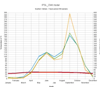
– IPSL Fig.28 :
•The temperature will increase on average of 2.1oC in the both future periods compared to the period 1970-1999.
•The beginning of wet season in the period 2046-2065 will be delayed by about fifteen days compared to the period 1970-1999 and the end of the wet season cor-responds approximatively to the end of wet season in the
16
Table 3 This table represents the year-averaged value of temperature and the year-amount value of precipitations on the three periods “1970-1999”, “2046-2065”and “2081-2100”for the INGV model in the sce-nario A1B. The arrows represents the evolution of the future value compared to the value of the past period.
Variable 1970-1999 2046-2065 2081-2100 Temperature (oC) 24.7 26.3 % 27.0 %
Precipitations (mm/an) 1501 1438 & 1478 &
period 1970-1999. The quantity of precipitations in the first seven months will be less of about 20% than the pe-riod 1970-1999 and in the rest of the year precipitations will increase of about 4%.
•The beginning of wet season in the period 2081-2100 will be delayed by about fifteen days compared to the period 1970-1999 and the end of the wet season cor-responds approximatively to the end of wet season in the period 1970-1999. Gobally, the quantity of precipi-tations of the first seven months of the year in the pe-riod 2081-2100 will be less of about 28% than the pepe-riod 1970-1999 and in the rest of the year precipitations will increase of about 25%, especially the second summit of precipitations which reach a monthly average of 591mm for September.
Table 4 This table represents the year-averaged value of temperature and the year-amount value of precipitations on the three periods “1970-1999”, “2046-2065”and “2081-2100”for the IPSL model in the sce-nario A1B. The arrows represents the evolution of the future value compared to the value of the past period.
Variable 1970-1999 2046-2065 2081-2100 Temperature (oC) 26.5 28.5 % 28.6 % Precipitations (mm/an) 1848 1753 & 1986 %
In conclusion for this scenario A1B, all of these three models are agree to say that the wet season will be delayed
Fig. 28 Same legend as the 26 but with the INGV model and be careful of the scale on this climagraph, the maximum of the precipitation scale is 600mm.
by about a ten days to one month and the summit of precip-itations of September-October will increase of 5% to 50% according to the model. All these three models are also agree with an increasing of temperature between 1.6oC and 2.5oC.
The three models are not agree with the end of wet season : the end of CCCMA-T47 is about fifteen days early than the period 1970-1999 and the end of the IPSL and INGV is the same. The three models are also not agree with the first summit of precipitions : The summit of precipitations of the CCCMA-T47 is higher (between 5% and 21%) than the summit of the period 1970-1999 whereas the summits of precipitations of the IPSL and INGV are lower (between 14% and 18%) than the summit of the period 1970-1999.
We can see below a discussion of the climographs and the year averages of each model for the future projection from the scenario A2 are :
– CCCMA-T47 :
•The temperature will increase on average of 1.8oC in the period 2046-2065 compared to the period
1970-17
1999 and will increase on average of 3.2oC in the period 2081-2100 compared to the period 1970-1999.
•The beginning of wet season in the period 2046-2065 will approximatively correspond to the begin of the wet season in the period 1970-1999 and the end of the wet season will be one month early compared to the pe-riod 1970-1999. On the other hand, the wet season will be more generous on the quantity of precipitations ; the late spring summit of precipitations increases of about 5% the late spring summit of precipitations increases of about 33%. The dry season is on average 13% more dry than the period 1970-1999.
•The beginning of wet season in the period 2081-2100 will be delayed by about fifteen days and the end of the wet season will be a few days early or approxima-tively correspond to the period 1970-1999. On the other hand, the wet season will be even more generous on the quantity of precipitations than the projection of the pe-riod 2046-2065 ; the first summit of precipitations in-creases of about 27%, the second one inin-creases of about 56% and on average on the whole wet season precipita-tions increase of 22%. The dry season is on average 13% drier than the period 1970-1999.
Table 5 This table represents the year-averaged value of temperature and the year-amount value of precipitations on the three periods “1970-1999”, “2046-2065”and “2081-2100”for the CCCMA-T47 model in the scenario A2. The arrows represents the evolution of the future value compared to the value of the past period.
Variable 1970-1999 2046-2065 2081-2100 Temperature (oC) 24.1 25.9 % 27.3 % Precipitations (mm/an) 1912 2019 % 2186 %
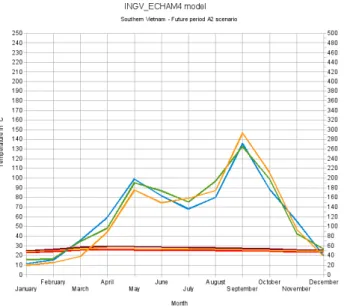
– INGV :
Fig. 29 Comparison of the climograph of the CCCMA-T47 model with the scenario A2 on different periods (1970-1999, 2046-2065 and 2081-2100) . The red line represents the temperatures on the period 1970-1999. The blue line represents the precipitations on the period 1970-1999. The yellow line represents the temperatures on the period 2046-2065. The green line represents the precipitations on the period 2046-2065. The brown line represents the temperatures on the period 2081-2100. The orange line represents the precipitations on the period 2081-2100.
•The temperature will increase on average of 1.4oC in the period 2046-2065 compared to the period 1970-1999 and will increase on average of 2.6oC in the period 2081-2100 compared to the period 1970-1999.
•The beginning of wet season in the period 2046-2065 will approximatively correspond to the begin of the wet season in the period 1970-1999 and the end of the wet season will be caracterised by a faster decrease of precipitations until they will reach a kind of thresh-old which is higher than the value of precipitations in the period 1970-1999. But we can considered that the end of the wet season is one month early. The quantity of precipitations during the dry season will be higher of 26% compared with the period 1970-1999. The quantity of precipitations during the two summits will be
approx-18
imatively the same as the period 1970-1999 but between these summits the precipitations will increase of about 13%.
•The beginning of wet season in the period 2081-2100 will be delayed by about one month compared to the period 1970-1999 and the end of the wet season cor-responds approximatively to the end of wet season in the period 1970-1999. Gobally, the quantity of precipi-tations of the first six months of the year in the period 2081-2100 will be less of about 22% than the period 1970-1999 and in the next five months the precipitations will increase of about 13%.
Fig. 30 Same legend as the 29 but with the INGV model
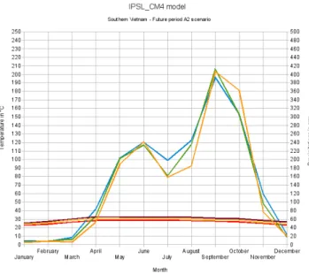
– IPSL :
•The temperature will increase on average of 1.8oC in the period 2046-2065 compared to the period 1970-1999 and will increase on average of 3.7oC in the period 2081-2100 compared to the period 1970-1999.
•The beginning of wet season in the period 2046-2065 will be delayed by about ten days compared to the period 1970-1999 and the end of the wet season will be
Table 6 This table represents the year-averaged value of temperature and the year-amount value of precipitations on the three periods “1970-1999”, “2046-2065”and “2081-2100”for the INGV model in the sce-nario A2. The arrows represents the evolution of the future value com-pared to the value of the past period.
Variable 1970-1999 2046-2065 2081-2100 Temperature (oC) 24.7 26.1 % 27.4 %
Precipitations (mm/an) 1501 1540 % 1465 &
also ten days early compared to the period 1970-1999. The quantity of precipitations during the wet season will be relatively the same as the period 1970-1999 however the period between the two summits of precipitations will decrease of about 8%.
•The beginning of wet season in the period 2081-2100 will be delayed by about fifteen days compared to the period 1970-1999 and the end of the wet season will be ten days early compared to the period 1970-1999. Globally, the quantity of precipitations during the wet season will be relatively the same as the period 1970-1999 however the period between the two summits of precipitations will decrease of about 15%.
Table 7 This table represents the year-averaged value of temperature and the year-amount value of precipitations on the three periods “1970-1999”, “2046-2065”and “2081-2100”for the IPSL model in the sce-nario A2. The arrows represents the evolution of the future value com-pared to the value of the past period.
Variable 1970-1999 2046-2065 2081-2100 Temperature (oC) 26.5 28.2 % 30.2 % Precipitations (mm/an) 1848 1762 & 1714 &
In conclusion for this scenario A2, all these three mod-els are agree with an increasing of temperature between 1.4oC and 3.7oC. These three models are not agree with the be-ginning or the end of the wet season and a model is not
19
Fig. 31 Same legend as the 29 but with the INGV model.
agree with the beginning or the end of the wet season de-pending of the future periode. But these three models are agree that the beginning is the same as the beginning of the period 1970-1999 or ten-fifteen days ahead and the end is the same as the period 1970-1999 or ten-fifteen days be-fore. All these three models are relatively agree with the september summit of precipitations : it will stay or increase in the future of about 0% to 56%. On the other hand, all these three models are not agree with the late spring sum-mit of precipitations. Indeed, it will be higher of 33% to 56% for the CCCMA-T47 model, but it will be lower or the same as the period 1970-1999 for the two other models. For the period 2046-2065, CCCMA-T47 and INGV are agree with an increase of precipitations (respectively 39mm and 107mm) whereas the IPSL decreases the precipitations dur-ing this period (86mm). For the period 2081-2100, INGV and IPSL are agree with a decrease of precipitations (re-spectively 36mm and 134mm) compared to the period 1970-1999 whereas the CCCMA-T47 model increases of 274mm the precipitations compared to the period 1970-1999.
We can see below a discussion of the climographs and the year averages of each model for the future projection from the scenario B1 are :
– CCCMA-T47 :
•The temperature will increase on average of 1.3oC
in the period 2046-2065 compared to the period 1970-1999 and will increase on average of 1.7oC in the period
2081-2100 compared to the period 1970-1999.
•The beginning of wet season in the period 2046-2065 will approximatively correspond to the begin of the wet season in the period 1970-1999 and the end of the wet season will be fifteen days early compared to the pe-riod 1970-1999. On the other hand, the wet season will be more generous on the quantity of precipitations ; the late spring summit of precipitations increases of about 13% and the late summer summit of precipitations in-creases of about 22%. On average on the whole wet sea-son precipitations decrease of 9%. The dry seasea-son is on average 18% drier than the period 1970-1999.
•The beginning of wet season in the period 2081-2100 will be delayed by about fifteen days and the end of the wet season will be a few days early or approx-imatively correspond to the period 1970-1999. On the other hand, the wet season will be even more generous on the quantity of precipitations than the projection of the period 2046-2065 ; the first summit of precipitations stays about the same value as the value of the period 1970-1999, the second one increases of about 24% and on average on the whole wet season the precipitations in-crease of 11%. The dry season is on average 15% drier than the period 1970-1999.
– IPSL :
•The temperature will increase on average of 1.5oC in the period 2046-2065 compared to the period
1970-20
Fig. 32 Comparison of the climograph of the CCCMA-T47 model with the scenario B1 on different periods (1970-1999, 2046-2065 and 2081-2100) . The red line represents the temperatures on the period 1970-1999. The blue line represents the precipitations on the period 1970-1999. The yellow line represents the temperatures on the period 2046-2065. The green line represents the precipitations on the period 2046-2065. The brown line represents the temperatures on the period 2081-2100. The orange line represents the precipitations on the period 2081-2100.
Table 8 This table represents the year-averaged value of temperature and the year-amount value of precipitations on the three periods “1970-1999”, “2046-2065”and “2081-2100”for the CCCMA-T47 model in the scenario B1. The arrows represents the evolution of the future value compared to the value of the past period.
Variable 1970-1999 2046-2065 2081-2100 Temperature (oC) 24.1 25.5 % 25.8 %
Precipitations (mm/an) 1912 1880 & 1976 %
1999 and will increase on average of 2.1oC in the period 2081-2100 compared to the period 1970-1999.
•The beginning of wet season in the period 2046-2065 will be delayed by about ten days compared to the period 1970-1999 and the end of the wet season will be the same as the period 1970-1999. The quantity of pre-cipitations during the wet season will be lower of about
6% than the period 1970-1999 however the late summer summit of precipitations will increases of about 14%.
•The beginning of wet season in the period 2081-2100 will be delayed by about fifteen days compared to the period 1970-1999 and the end of the wet season will be the same as the period 1970-1999. Globally, the quan-tity of precipitations during the wet season will be lower of 14% than the period 1970-1999 and the dry season will be relatively the same as the dry season of the pe-riod 1970-1999.
Fig. 33 Same legend as the 32 but with the INGV model.
Table 9 This table represents the year-averaged value of temperature and the year-amount value of precipitations on the three periods “1970-1999”, “2046-2065”and “2081-2100”for the IPSL model in the sce-nario B1. The arrows represents the evolution of the future value com-pared to the value of the past period.
Variable 1970-1999 2046-2065 2081-2100 Temperature (oC) 26.5 28.0 % 28.6 %
21
In conclusion for this scenario B1, these two models are agree with an increasing of temperature between 1.3oC and 2.1oC. These two models are agree that the beginning is the same as the beginning of the period 1970-1999 or ten-fifteen days ahead and the end is the same as the period 1970-1999 or ten-fifteen days before. These two models are also agree with the decreasing between 5% and 18% of pre-cipitations on all periods, especially during the dry season where the decreasing of precipitations is on average 24%. Concerning the future trend of the wet season, these two models are not agree and one model is not agree depend-ing the future projection periods. Indeed, the CCCMA-T47 model the wet season increases of 2% for the period 2046-2065 and 4% for the period 2081-2100, and the IPSL model the wet season decreases of 6% for the period 2046-2065 and 14% for the period 2081-2100.
In conclusion for this part, the Table 16 and Table 17 compile all the results. We can see that all the models are unanimous with an delaying of the beginning of the wet sea-son. The evolution of the end of the period is less obvious, the general trend is ahead compared to the past period, but the models tend to be relatively close from the date of the past period. Concerning the late summer summit of precip-itation, the models tend to increase it. The annual mean of temperature tends to increase in the future and all models are unanimous to this fact. However, concerning the late spring summit of precipitations and the annual amount of precipi-tations, the models are not agree among themselves.
Beginning and End of the wet season
Unlike the precedent method to evaluate the beginning and the end of the wet season. Here, we calculate more pre-cisely the beginning and the end of the wet season for each model and each scenarios. For this aim, we determine the
Julian-day during the year and the moving average on one week (-3 days, the day and +3 days). We define the begin-ning of the wet season as the Julian-day which the moving average of the 3 last days are below the threshold of 2 mm of precipitations and the 20 next days are above the threshold of 2 mm of precipitations. The threshold of 2 mm of precip-itations is defined in [MANTON et al. 2001] as a rainy day. And we define the end of the wet season as the Julian-day which the moving average of the 3 last days are above the threshold of 2 mm of precipitations and the 20 next days are below the threshold of 2 mm of precipitations. Sometimes these conditions are not reached, so the year is not take in account and equal zero in the detailed list of the years.
– CCCMA-T47 :
•The beginning of the wet season 34 for this model is delayed of 1 to 13 days whatever the future period or the scenario considered. For the scenarios A1B and B1, the delay increases in the far future compared to the near future. For the scenario A2, the delay is similar on both future periods.
•The end of the wet season 35 for this model is am-biguous. For the scenario A1B, the end of the wet season will be in advance of 4 days in the near future and de-layed of 1 day in the far future. For the scenario B1, the end of the wet season will be delayed of 7 days in the near future and of 1 day in the far future. For the sce-nario A2, the end will be approximatively the same as the past period.
– INGV :
•The beginning of the wet season 36 for this model is delayed of 16 to 23 days whatever the future period or the scenario considered. For the scenarios A1B, the delay increases in the near future of 20 days and in the
22
Fig. 34 Comparison of the beginnings of the wet season of the model CCCMA-T47 over the past period (blue bar) and the future periods 2046-2065 (red bar) and 2081-2100 (yellow bar) and with the 3 sce-narios A1B, A2 and B1.
far future of 23 days. For the scenarios A2, the delay in-creases in the near future of 18 days and in the far future of 16 days.
•The end of the wet season 37 for this model is am-biguous. For the scenario A1B, the end of the wet season will be in advance of 8 days in the near future and de-layed of 5 days in the far future. For the scenario A2, the end of the wet season will be delayed of 3 days in the near future and of 4 days in the far future.
– IPSL :
•The beginning of the wet season 38 for this model is delayed of 1 to 10 days whatever the future period or the scenario considered. For the scenarios A1B, the delay increases in the near future of 10 days and in the far future of 6 days. For the scenarios A2, the delay in-creases in the near future of 1 days and in the far future of 6 days. For the scenarios B1, the delay increases in the near future of 2 days and in the far future of 7 days.
Fig. 35 Comparison of the ends of the wet season of the model CCCMA-T47 over the past period (blue bar) and the future periods 2046-2065 (red bar) and 2081-2100 (yellow bar) and with the 3 sce-narios A1B, A2 and B1.
23
Fig. 37 Same legend as the 35 but with the INGV model.
Fig. 38 Same legend as the 34 but with the IP model.
•The end of the wet season 39 for this model is ad-vanced of 2 to 8 days whatever the future period or the scenario considered. For the scenario A1B, the end of
the wet season will be in advance of 2 days in the near future and advanced of 4 days in the far future. For the scenario A2, the end of the wet season will be advanced of 8 days in the near future and of 5 days in the far fu-ture. For the scenario B1, the end of the wet season will be advanced of 5 days in the near future and of 3 days in the far future.
Fig. 39 Same legend as the 35 but with the IPSL model.
In conclusion for the beginning of the wet season, the models are unanimous : The beginning of the wet season will be delayed of 1 to 20 days according to the models, the period and the scenario.
In conclusion for the end of the wet season, the mod-els are not agree among themselves. Only the IPSL model
24
is agree to itself with the 3 scenarios : the end of the wet season will be ahead to 2 to 8 days. The two others models are not agree with itself and none conclusion can be extract.
7 Discussions
As said in the Chapter 5 the second sorting, it is important to moderate the IPSL model. Indeed, this model overestimates the late summer summit of precipitations in the past and also the temperatures all over the year. However, the late summer summit of precipitations is not excessive in the Climographs analysis, the evolution of this summit in the IPSL model is less than the evolution of the summit of the CCCMA-T47 model. Concerning, the evolution of temperatures, the IPSL contains the highest range of value for both future periods. This overestimating of the temperature is about 14%. If we decrease the range of the IPSL of 14%, we obtain approxi-matively the same range as the CCCMA-T47 model.
We can see that for the past period, the models do not represent exactly the climate in one region, this fact implies that the models do not represent exactly the future climate in one region. Thus, the most important results are the global trend of the projections given by model and the range of the evolution of the value range of a climate variable. The abso-lute value of a daily future climate variable is very danger-ous to use because the probability to obtain this prediction during the relevent day is very infime. The absolute value of a monthly mean variable is more probabel but still risky.
It is important to keep in mind that all of these results come from models with different spatial resolutions and these spatial resolutions are different from a model to another. This means that the interpolation on the subjacent region is different from a model to another. An other important detail is the fact that the precipitations are the one of the variables
the most difficult to forecast because the precipitations are discontinuous fields and the variability in space and time of this cariable are large. This fact imply that if the model have a large spatial resolution, the results in the precipitations will be affected.
We also must keep in mind that the reanalysis models also have the disadvantages of models in general. The results is also influenced by the spatial and temporal resolution of the model and the interpolation on the subjacent region is different from a resolution to another. But the results over a region also depend of the observationnal data which are forced inside the reanalysis model. We compare the IPCC models to the reanalysis models because we only have these data as continuous real observations.
8 Conclusions
This work analyses the future climate over the region of the province of Binh Thuan in South Vietnam from the IPCC Model. To reach this aim, we must select the models which best represent the reality and analyse the future projections of these selected models. We use the reanalysis models as the best representation of the reality we have. The selection is based on two sorting : The first is the comparison of climo-graphs between the IPCC models with a range of ±2σ of the reanalysis models and the second is the comparison of the variables of precipitations and temperatures between IPCC models with a range of ±1σ . After these two sortings, three models are selected : CCCMA-T47, INGV and IPSL.
The future projection analysis is based on three steps : The first is the analysis of the basic climate statistics, the second is the analysis of the climographs and the third is the analysis of the beginning and end of the wet season:
25
– The first analysis indicates an increase of temperature, an increase of the days which are lower than 2 mm of daily precipitations (decrease of the sum of events of consecutive days which are lower than 2 mm of daily precipitations but increase of the sum of days inside one event) and an increase of extreme temperature and ex-treme precipitations. This first analysis is not conclusive concerning the evolution of the annual amount of pre-cipitations.
– The second analysis indicates a delaying of the begin-ning of the wet season, the end of the wet season is ahead for this analysis, the late summer summit of pre-cipitations increases compared to the past period and the annual mean of temperature also increases. Concerning the late spring summit of precipitations and the annual amount of precipitations, this analysis can not concluded a general trend because the models are not agree with themselves.
– This third analysis indicates a delaying of the beginning of the wet season of 1 to 20 days according to the mod-els, the period and the scenario. But this analysis can not concluded a general trend because the models are not agree with themselves, only the IPSL is agree with itself and proposes an advance of the end of the wet season.
We must nuance these conclusions with the remarks in the discussion section. Indeed, all of the models (IPCC mod-els and Reanalysis modmod-els) presented in this work have dif-ferent spatial resolutions. So the interpolation of data over the subjacent region will be affected by this spatial resolu-tions. The past period is not pretty good represented by the selected IPCC models, so we can think that in the future, it will probably not be the case either. And finaly, we must keep in mind that the precipitations are the climate variables
among the most difficult to predict.
Acknowledgements We thank the European Center for Medium-Range Weather Forecasts (ECMWF) for the ERA-40 reanalysis and the opera-tional analysis data (http://www.ecmwf.int/) and the NOAA/OAR/ESRL PSD (Boulder, Colorado, US) for the NCEP/NCAR Reanalysis (http:// www.cdc.noaa.gov/).
References
IPCC AR4-WGI 2007. IPCC (2007) In: Solomon S, Qin D, Manning M, Chen Z, Marquis M, Averyt KB, Tignor M, Miller HL (eds) Climate change 2007: The physical Science Basis. Contribution of Working Group I to the Fourth Assessment Report of the Intergov-ernmental Panel on Climate Change. Cambridge University Press, Cambridge, United Kingdom and New York, NY, USA
LELOUP et al. 2007. Leloup J., Lengaigne M., Boulanger J.P. (2007) Twenty Century ENSO characteristics in the IPCC data base. Cli-mate Dynamics 30:277-291, doi:10.1007/s00382-007-0284-3 MANTON et al. 2001. M.J. MANTON, P.M. DELLA-MARTA, M.R.
HAYLOCK, K.J. HENNESSY, N. NICHOLLS, L.E. CHAMBERS, D.A. COLLINS, G. DAW, A. FINET, D. GUNAWAN, K. INAPE, H. ISOBE, T.S. KESTIN, P. LEFALE, C.H. LEYU, T. LWIN, L. MAITREPIERRE, N. OUPRASITWONG, C.M. PAGE, J. PAHA-LAD, N. PLUMMER, M.J. SALINGER, R. SUPPIAH, V.L. TRAN, B. TREWIN, I. TIBIG and D. YEE (2001) Trends in extreme daily rainfall and temperature in Southeast Asia and the South Pacific: 19611998. International journal of Climatology, Int. J. Climatol. 21: 269284 (2001), DOI: 10.1002:joc.610
NIEUWOLT S., 1981. NIEUWOLT S. (1981) The climates of con-tinental Southeast Asia. World Survey of Climatology Volume 9 : Climates of southern and western Asia, ed. by LANDSBERG H.E., TAKAHASHI K. and ARAKAWA H., Elsevier, Amsterdam-Oxford-New-York
26 Table 10
CCCMA-T47 model Past Scenario A1B Scenario A2 Scenario B1 Variables 1970-1999 2046-2065 2081-2100 2046-2065 2081-2100 2046-2065 2081-2100 Mean Temperature (C) 24,1 25,74 26,57 25,92 27,34 25,45 25,78 Sum Precipitation (mm/year) 1911,88 1990,47 1955,17 2019,51 2186,22 1879,96 1976,21 Standard-Error Temperature (C) 3,6 4,21 4,2 4,11 4,23 4,07 4,1 Standard-Error Precipiation (mm) 9,64 10,32 10,56 4,11 13,2 8,72 10,22
Maximum Temperature (C) 30,47 33 34,08 32,16 34,5 32,84 32,96 Minimum Temperature (C) 13,28 16,38 16,16 14,75 16,47 14,38 15,62 Maximum Precipitation (mm) 171,39 193,11 149,61 170,47 186,12 146,22 166,98 Centile 50 of the Temperature (C) 24,26 25,89 26,64 26,02 27,43 25,56 25,86 Centile 50 of the Precipitation (mm) 2,29 2,12 1,95 2,07 1,99 2,09 2,19
Centile 99 of the Temperature (C) 28,43 30,19 31,44 30,55 32,15 29,84 30,52 Centile 99 of the Precipitation (mm) 49,05 52,57 53,77 54,47 71,13 45,82 54,72
Table 11
CCCMA-T47 model Past Scenario A1B Scenario A2 Scenario B1 Persistance of less than 2mm 1970-1999 2046-2065 2081-2100 2046-2065 2081-2100 2046-2065 2081-2100
Sum of events over 10 years 304 289 299 287 275 296 287 Mean of days in one event 5,76 6,21 6,15 6,28 6,63 6,07 6,22 Maximum days in one event 93 75 84 93 101 93 121 Sum of days in event over 10 years 1750 1794 1838 1801 1824 1796 1786
27 Table 12
INGV model Past Scenario A1B Scenario A2 Variables 1970-1999 2046-2065 2081-2100 2046-2065 2081-2100 Mean Temperature (C) 24,7 26,31 26,95 26,12 27,38 Sum Precipitation (mm/year) 1458,76 1438,1 1478,36 1540,2 1465,11 Standard-Error Temperature (C) 3,36 3,98 4,02 3,93 4,08 Standard-Error Precipiation (mm) 7,08 7,48 8,19 3,93 8,29 Maximum Temperature (C) 29,84 31,75 33,67 31,74 34,2 Minimum Temperature (C) 17,88 18,69 18,92 19,32 19,63 Maximum Precipitation (mm) 218,51 102,97 171,45 115,53 176,29 Centile 50 of the Temperature (C) 24,7 26,29 26,85 26,1 27,3 Centile 50 of the Precipitation (mm) 0,97 0,8 0,69 0,96 0,68 Centile 99 of the Temperature (C) 28,31 30,34 31,36 30,23 32,08 Centile 99 of the Precipitation (mm) 27,97 32,96 35,01 35,15 34,86
Table 13
INGV model Past Scenario A1B Scenario A2 Persistance of less than 2mm 1970-1999 2046-2065 2081-2100 2046-2065 2081-2100
Sum of events over 10 years 462 458 435 450 433 Mean of days in one event 4,68 4,97 5,31 4,87 5,29 Maximum days in one event 81 97 79 96 143 Sum of days in event over 10 years 2162 2274 2309 2190 2291
28 Table 14
IPSL model Past Scenario A1B Scenario A2 Scenario B1 Variables 1970-1999 2046-2065 2081-2100 2046-2065 2081-2100 2046-2065 2081-2100 Mean Temperature (C) 26,46 28,53 28,62 28,28 30,16 27,98 28,62 Sum Precipitation (mm/year) 1781,52 1753,5 1860,12 1761,67 1713,65 1779,08 1693,61 Standard-Error Temperature (C) 3,92 4,47 4,52 4,45 4,55 4,46 4,52 Standard-Error Precipiation (mm) 7,04 8,75 12,24 4,45 9,25 7,95 7,44 Maximum Temperature (C) 32,5 35,87 36,81 35,87 37,1 35,06 36,81 Minimum Temperature (C) 15,21 18,01 13,37 17,82 18,99 17,12 13,37 Maximum Precipitation (mm) 123,7 218,25 266,07 253,79 280,03 174,88 150,98 Centile 50 of the Temperature (C) 27,35 29,33 29,46 29,1 30,99 28,87 29,46 Centile 50 of the Precipitation (mm) 3,3 2,29 1,83 2,38 1,77 2,66 2,1
Centile 99 of the Temperature (C) 29,8 33,81 33,77 32,26 35,37 32,31 33,77 Centile 99 of the Precipitation (mm) 29,6 32,34 44,63 34,59 35,2 34,32 31,65
Table 15
IPSL model Past Scenario A1B Scenario A2 Scenario B1 Persistance of less than 2mm 1970-1999 2046-2065 2081-2100 2046-2065 2081-2100 2046-2065 2081-2100
Sum of events over 10 years 126 141 158 152 165 141 155 Mean of days in one event 12,89 12,45 11,58 11,37 11,18 12,03 11,47 Maximum days in one event 149 171 172 157 170 166 170 Sum of days in event over 10 years 1624 1756 1829 1727 1844 1695 1777
29 Table 16 Summary table of the results of the analysis of the
climo-graphs on the three models on the period 2046-2065. The evolution is represented by the arrows refer to the past period and the range is cre-ated by the minimum and maximum value of the analysis. A ↑ means that the evolution is strictly positive. A % means that the evolution is positive or equal to zero. A → means that the evolution is equal to zero. A & means that the evolution is negative or equal to zero. A ↓ means that the evolution is strictly negative. A ∅ means that the evolution has no general trend.
2046-2065 CCCMA-T47 INGV IPSL Beginning of the wet
season (days)
% % ↑
[0 : +10] [0 : +10] [+10 : +15] Ending of the wet
season (days)
↓ & & [−30 : −10] [−30 : 0] [−10 : 0] Late spring summit of
precipitation (%)
↑ ↓ &
[+5 : +20] [−11 : −4] [−4 : 0] Late summer summit
of precipitation (%) ↑ ∅ ↑ [+15 : +33] [−2 : +10] [+5 : +14] Annual sum of precipitation (%) ∅ ∅ ↓ [−2 : +6] [−4 : +3] [−5 : −4] Annual mean of temperatures (oC) ↑ ↑ ↑ [+1.3 : +1.8] [+1.4 : +1.6] [+1.5 : +2.1]
30
Table 17 Same legend as the 16 but with the period 2081-2100.
2081-2100 CCCMA-T47 INGV IPSL Beginning of the wet
season (days)
↑ ↑ ↑
[+10 : +15] [+30] [+15] Ending of the wet
season (days)
& → & [−10 : 0] [0] [−10 : 0] Late spring summit of
precipitation (%)
↑ & ↓
[0 : +27] [−14 : −11] [−18 : −1] Late summer summit
of precipitation (%) ↑ ↑ ∅ [+24 : +56] [+8 : +13] [−3 : +50] Annual sum of precipitation (%) ↑ ↓ ∅ [+2 : +14] [−2] [−8 : +1] Annual mean of temperatures (oC) ↑ ↑ ↑ [+1.7 : +3.2] [+2.2 : +2.6] [+2.1 : +3.7]


![Risiko- & [und] Schutzfaktoren der psychischen Gesundheit humanitärer Einsatzhelfer : eine systematische Literaturübersicht](data:image/gif;base64,R0lGODlhAQABAIAAAP///wAAACH5BAEAAAAALAAAAAABAAEAAAICRAEAOw==)