Astronomy& Astrophysics manuscript no. sl_light © ESO 2017 May 5, 2017
Analysis of luminosity distributions of strong lensing galaxies:
subtraction of diffuse lensed signal
J. Biernaux
1, P. Magain
1, and C. Hauret
1Université de Liège
STAR Research Unit - OrCA Group Quartier Agora. Bât. B5c Allée du 6 Août, 19c B-4000 Liège 1 (Sart-Tilman) Belgique [email protected] [email protected] [email protected] May 2017 ABSTRACT
Context.Strong gravitational lensing gives access to the total mass distribution of galaxies. It can unveil a great deal of information about the lenses’ dark matter content when combined with the study of the lenses’ light profile. However, gravitational lensing galaxies, by definition, appear surrounded by lensed signal, both point-like and diffuse, that is irrelevant to the lens flux. Therefore, the observer is most often restricted to studying the innermost portions of the galaxy, where classical fitting methods show some instabilities.
Aims.We aim at subtracting that lensed signal and at characterising some lenses’ light profile by computing their shape parameters (half-light radius, ellipticity, and position angle). Our objective is to evaluate the total integrated flux in an aperture the size of the Einstein ring in order to obtain a robust estimate of the quantity of ordinary (luminous) matter in each system.
Methods.We are expanding the work we started in a previous paper that consisted in subtracting point-like lensed images and in independently measuring each shape parameter. We improve it by designing a subtraction of the diffuse lensed signal, based only on one simple hypothesis of symmetry. We apply it to the cases where it proves to be necessary. This extra step improves our study of the shape parameters and we refine it even more by upgrading our half-light radius measurement method. We also calculate the impact of our specific image processing on the error bars.
Results.The diffuse lensed signal subtraction makes it possible to study a larger portion of relevant galactic flux, as the radius of
the fitting region increases by on average 17%. We retrieve new half-light radii values that are on average 11% smaller than in our previous work, although the uncertainties overlap in most cases. This shows that not taking the diffuse lensed signal into account may lead to a significant overestimate of the half-light radius. We are also able to measure the flux within the Einstein radius and to compute secure error bars to all of our results.
Key words.Galaxies: elliptical, luminosity function. Gravitational lensing: strong
1. Introduction
Gravitational lensing is a powerful tool to address many astrophysical questions, ranging from cosmology to galaxy formation and evolution, as it offers a precise technique for studying mass distributions in general. Strong lensing, in particular, gives access to valuable information about galactic mass profiles. In the case of early-type galaxies, as the study of their dynamics is rather challenging, especially at high-z (Romanowsky et al. 2003; Cappellari et al. 2015), strong lensing practically constitutes our only proxy for the mass distributions. Luckily, thanks to their usually higher surface mass density, elliptical galaxies are more often involved in gravitational lensing phenomena than spirals. While strong lensing offers a possibility of understanding their total mass distribution, comparing it to their brightness profile could provide valuable information about dark matter in early-type galaxies (Bertin et al. 1994; Romanowsky et al. 2003; Dekel et al. 2005; Cappellari et al. 2015). It is therefore of highest interest to accurately determine the luminosity distribution of
lensing galaxies.
However, the existence of lensed images around a galaxy makes the study of its light profile troublesome. Indeed, the deflected light from the background source produces point-like and diffuse components that act as a parasite signal when one wants to access only the lens brightness. The authors address this issue in Biernaux et al. (2016) (hereafter B16) by implementing a careful subtraction of the point-like lensed images for seven gravitational lensing systems from the CfA-Arizona Space Telescope LEns Survey (CASTLES) database (Muñoz et al. 1998). A precise point-spread function (PSF) determination is necessary for achieving a good point sources subtraction. Like many authors who have processed lenses in the framework of the COSmological MOnitoring of GRAvItational Lenses (COSMOGRAIL) project (Chantry et al. 2010; Courbin et al. 2011; Sluse et al. 2012), we use the MCS deconvolution algorithm (Magain et al. 1998; Chantry & Magain 2007). It is well suited to gravitational lensing images, as it consists
in iteratively subtracting a diffuse component, including any non-point-like object, such as galaxies and lensed arcs, until convergence to an image of the point sources. Moreover, it has the important advantage of not violating the sampling theorem. In B16 as well as in Chantry & Magain (2007) or Chantry et al. (2010), we explain that other PSF determinations, using, for example, the TinyTim software (Hook & Krist 1997; Krist & Hook 1997), are not accurate enough to perform such a subtraction.
Nonetheless, even after PSF subtraction, the uncertainties in the outer regions of the galaxy restrain the modelling of the light profile to its inner regions. It is shown in B16 that classical fitting techniques such as GALFIT (Peng et al. 2002, 2010) perform poorly in these conditions. We also tackle that problem in B16 by implementing an innovative study of the shape parameters of lensing galaxies, that is, the position angle (PA) of the galaxy major axis, its ellipticity (ε), and its half-light radius (reff). We design a method that is not too sensitive to the above-mentioned artefacts: we propose to study each of them individually, so as to avoid the existence of local minima in the parameters space. The basis of this modelling is the computation of isophotes. We show in B16, from simulations, that our reff measurement technique, which we call the linear regression method (LRM), is more trustworthy than GALFIT in the case of lensing galaxies. The latter shows instabilities regarding the fitting region, but also crucial aspects of image processing, such as the PSF or the signal-to-noise ratio (S/N). We also show that our technique is better-suited for galaxies that are not much larger than the PSF, which comes in handy for lensing images, as we often deal with only the inner parts of the lens. Moreover, the LRM depends less on the value of the Sérsic index of the model we choose to represent the galaxy. We thus obtain reliable reffvalues and present all the results in a CDS (Centre de Données astronomiques de Strasbourg) table1 (Biernaux et al. 2015) associated to B16.
In this work, we expand the study of the B16 sample. Despite the point-source subtraction, some diffuse lensed signal, in the form of arcs or a ring surrounding the lenses, remains as a nuisance to the study of their light profile. We aim at designing a method to subtract that signal, in order to be able to encompass more of the outer parts of the galaxy in the fitting region. As the value of reff is sensitive to the wings of the galaxy light profile, this constitutes an improvement to the B16 reff. We also improve the LRM by switching to a χ2 validity criterion for the linear regression. Since the initial motivation of this work is to compare light distributions to total mass distributions of lensing galaxies, we finally compute the integrated flux within the Einstein radii of our lenses.
This paper is structured as follows. In Sect. 2, we give some information about our sample. In Sect. 3, we explain the addi-tions and improvements to the B16 shape parameters measure-ment methods that we implemeasure-ment. We discuss the errors in Sect. 4 and eventually apply it to our sample, discussing the results in Sect. 5. We give a short conclusion in Sect. 6.
1
http://vizier.cfa.harvard.edu/viz-bin/VizieR?-source=J/A+A/585/A84
2. Data
We are processing the same data as in B16, where a complete and illustrated description of our sample can be found. In short, our dataset is a seven-systems subsample from the data pro-cessed in Chantry et al. (2010) and Sluse et al. (2012), from the CASTLES database (Muñoz et al. 1998). Their selection crite-ria were that the systems should have securely known redshifts for both the lens and the background quasar and they excluded systems with multiple lenses of similar luminosity. As in B16, we are focusing on quadruply-imaged sources, thus reducing the full sample to our seven systems. The images were obtained with the NIC2 camera of the Near Infrared Camera and Multi-Object Spectrometer (NICMOS) instrument onboard the Hubble Space Telescope (HST) between 1997 and 2004 in the near infrared H-band. The angular scale of these images is 0.075 arcseconds per pixel. Table 1 summarises the systems coordinates and red-shifts. We use astrometrical results from Chantry et al. (2010) and Sluse et al. (2012), as well as their accurate PSFs.
3. Methods 3.1. Pre-processing
A complete walk-through of the pre-processing can be found in B16. To sum up, after the common poor quality pixels cleanup and the sky subtraction, a point source subtraction has been con-ducted on the data frames. Indeed, with the purpose of disen-tangling signal from the lensed point-like components and from the galaxy, that subtraction consists in building an image of the four point sources, taking the PSF into account, and subtracting it directly from each data frame.
3.2. Subtracting the diffuse lensed component
The first aim of this work is to extend the lensed signal sub-traction to the arc. Similarly to the subsub-traction of the point-like images, we aim at building an image of the arc and at directly subtracting it from the original data frame. We formulate only one simple hypothesis: because the arc consists of an image of the background galaxy, its light distribution displays, to the first order, the same properties of radial symmetry. In other words, along a galactocentric radius, the arc should have a symmetric light distribution on either side of its maximum intensity.
In order to compute the arc radial light distribution, we first locate the maximum intensity of the arc with respect to the centre of our lens. We choose to work in a galactocentric coordinate system. For a few azimutal coordinates θ (typically about 200, evenly distributed around the whole ring), we locate the pixel with the highest intensity in the arc. This yields an ensemble of (rmax ; θ) datapoints, rmax being the distance between that pixel and the galactic centre. To refine the location of rmax, we fit a constant plus a linear combination of sines up to the second order on these datapoints:
rmax(θ)= rmax0 + a1sin(θ)+ a2sin(θ2), (1) where r0
max is the average of rmax. We actually conduct this operation separately on pieces of the arc between pairs of point sources. We exclude coordinates where PSF subtraction has been performed. We thus get a function rmax(θ) that locates the centre of symmetry of the arc light profile at any angle. We divide the arc image into sectors of various sizes along the angular coordinate, as shown in the left panel of Fig. 1. Within
Table 1: List of the systems that have been processed in B16 and in this work.
System # frames Source redshift Lens redshift RA (J2000) DEC (J2000)
MG0414+0534 13 2.64 0.96 04:14:37.73 +05:34:44.3 HE0435-1223 4 1.689 0.46 04:38:14.9 −12:17:14.4 RXJ0911+0551 4 2.80 0.77 09:11:27.50 +05:50:52.0 SDSS0924+0219 8 1.524 0.359 09:24:55.87 +02:19:24.9 PG1115+080 4 1.72 0.351 11:18:17.00 +07:45:57.7 SDSS1138+0314 4 2.44 0.45 11:38:03.70 +03:14:58.0 B1422+231 4 3.62 0.354 14:24:38.09 +22:56:00.6
Fig. 1: Left: sketch of the division of an image of HE0435-1223 into sectors along the angular coordinates. Right: collapsed radial profile of a sector from HE0435-1223. The crosses represent the measured intensity along the radial coordinate. The solid line shows the best-fitting de Vaucouleurs profile regarding the residuals maximum symmetry criterion.
each sector, we require rmaxto not vary more than a few percent. However, should rmax(θ) be nearly constant, the maximum angular width of a sector is set to a value chosen by the user, typically around 20 degrees. The width of sectors is therefore a parameter of the arc subtraction process, but its influence on the arc subtraction is negligible compared to the other sources of systematics considered in our error calculation (Sect. 4).
The next step consists in collapsing the 2-D image of the arc into 1-D radial profiles. This is done by re-scaling the length of all the rows of pixels of the same angular coordinate, also called traces, within each sector so that they get the exact same rmax. Then, the re-scaled traces are summed and averaged. The result-ing radial profile, shown in the right panel of Fig. 1, corresponds to the sum of the galaxy and the arc radial profiles, the latter showing up as a "bump" around rmax. We model the galaxy pro-file I(r) as a de Vaucouleurs law,
I(r)= I0exp −k r reff !1/4 , (2)
where I0 is the central pixel intensity, reff the half-light radius and k a normalisation constant. This expression is valid for a centred light distribution, which is the case in our galactocentric coordinate system. It is also valid for a circular galaxy. However, we consider the ellipticity of the lens by using r = √(ab) as a radial coordinate, where a and b are respectively the semi-major and semi-minor axes. We use as a validity criterion that the de Vaucouleurs profile parameters maximise the symmetry of the residuals in a given region of interest around rmax. The solid curve on Fig. 1 gives an example of the galactic profile giving the most symmetric residuals wings around
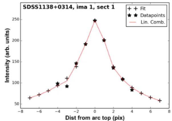
rmax. Those residuals act as datapoints for the arc radial light profile. The size of the region of interest is also a parameter of the process: the larger the better, but not so large that we mis-takenly consider parts of the image where there should be no arc. Although it is valid to the first order, the hypothesis of sym-metry around rmax may not always apply perfectly. Moreover, our symmetry criterion is more stable when restricted closer to the arc maximum, where the signal clearly dominates the noise. To extend the arc estimate to lower intensities, we fit a de Vaucouleurs law on each of the arc wings. We then compute a linear combination (per wing) of the fitted values and the datapoints, with weights so that the datapoints dominate around the centre of symmetry and the fitted values dominate closer to the wings (see Fig. 2). That way we obtain a numerical profile that is a close approximation of the true arc radial light distribution.
Finally, for each trace within the sector, we scale that numerical profile to better fit the radial intensities of each angular coordinate. We repeat the process on each sector, yielding for each one a numerical radial profile of the arc. We end up with as many arc profiles as traces, each corresponding to a single angular coordinate. We thus have a map of the arc intensity as a function of galactocentric coordinates (r, θ). To reconstruct a 2-D image of the arc in cartesian coordinates, we compute the intensity of each pixel by interpolating on its direct neighbours on that map. Finally, we can subtract that 2-D image from the data frame. The arc subtraction has been performed on each individual image of four out of seven galaxies in our sample. Indeed, on the remaining three systems, there was no visible diffuse lensed signal contaminating the galaxy light, no
Fig. 2: Two examples of numerical radial profile computation for one sector of the arc of HE0435-1223 and from SDSS1138+0314. The stars picture the datapoints for the arc radial light profile. The crosses represent the best fitting de Vaucouleurs models for each wing. The solid line shows the linear combination that acts as the arc numerical profile.
significant "bump" in their radial profile. The results are shown in Fig. 3. Once all the lensed signal, both point-like and diffuse, has been subtracted from the data frames, we can proceed to the shape parameters measurement, as explained in Sect 3.3.
3.3. Measuring the shape parameters
The second aim of this work is to compute, with the highest possible accuracy, the shape parameters of the lenses (the PA, ε, and reff). Each parameter has been calculated individually, in order to avoid the problem of potential local minima in the parameters space. The methods are described in great details in B16. Since the publication of that paper, we have added the arc subtraction to the pre-processing of our sample. Therefore, we conducted those measurements again. The results remain unchanged for the position angle and the ellipticity. An extensive description of those parameters’ measurements, can be found in B16 and in the associated table summarising our results on the CDS website (Biernaux et al. 2015). However, we have slightly modified the reff measurement method, improved its values, and computed a more secure error bar.
In B16, the LRM was based on determining the slope of a lin-ear relationship between ln I and r1/4, defined by the logarithm of Eq. 2; ln I = ln I0− k r reff !1/4 (3) assuming a de Vaucouleurs brightness distribution. The ra-dial profile of each lens has been obtained by computing its isophotes, using one-pixel-wide masks of increasing semi-minor axis. Then, a de Vaucouleurs profile convolved by the instrument PSF was generated and its shape parameters were fine-tuned until the slope of this synthetic lens in the (ln I ; r1/4) space matches the measured slope on the data frame. In this work, we have chosen to proceed in a similar way, only we do not use the slope of ln I(r1/4) as a validity criterion for the model. Instead, we adjust the shape parameters until they minimise the χ2 between the datapoints and the convolved model radial profile in the (ln I ; r1/4) space. Because we do not have any information about I0 at that point, for each try, the convolved model logarithmic profile is translated by a constant (∆) that is
an average of the difference between matching datapoints from the convolved model and the data frame radial profiles. This process is less time-consuming than the LRM and we find it to be more trustworthy as it grants less importance to the outliers. In conclusion, even though the arc intensity is not dominant in the portion of the galaxy that is taken into account for the reff measurement, it still produces some contamination. Thanks to the arc subtraction, that contamination is removed and more points in the outer parts of the lens galaxy can be taken into ac-count for the computation of its radial profile, which improves the reffmeasurement, as discussed in Sect 5. The region of inter-est for this new LRM is shown in Fig. 5. As in B16, its radius is determined visually by the user. The reff values obtained in B16 have been updated, as listed in Table 2.
3.4. Computing the integrated luminosity within the Einstein radius
The final aim of this work is to calculate the integrated flux in the H-band within the Einstein radii rE of our seven lenses. We used the rE values from Sluse et al. (2012), more specifically, from their Table 7. We list them in Table 3.
Similarly to what is performed for the shape parameters, we aim at a simple, 1-D measurement method for the central inten-sity parameter I0; we scan a wide interval of I0values and refine it until it minimises the∆ translation constant between the model and the data radial profiles. Once in possession of the correct I0 value, we can produce an image of the deconvolved galaxy profile, which is thus the best analytical model of the lensing galaxy brightness distribution. This is the image that we use to compute the integrated flux within the Einstein radius FH. The measurement is simply performed by integrating the total signal in an aperture centred on the lens of a radius equal to rE, then converting this value into an H-band flux, taking into account the instrument gain, exposure time, and a K-correction. The latter corrects from the offset between the redshifted lens spectrum and the NICMOS instrument bandpass, and is computed based on an elliptical galaxy template spectrum synthesised using the Pégase software (Fioc & Rocca-Volmerange 1997). The K-correction results as a factor K such that FH = KFλ, where Fλis the measured flux and FHis the corrected flux. All three
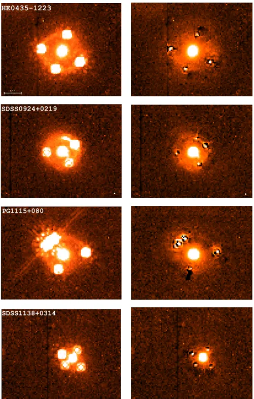
Fig. 3: Left: HST-NICMOS data frames from our samples. Right: resulting images after the lensed signal subtraction, point sources and arcs. Only one data frame is shown for each system and only for the systems on which the arc subtraction has been conducted.
values are given for each system in Table 3. We also give FH expressed in solar units, using a value of FH, (Colina et al. 1996) at the distance of each lens for a WMAP (Lewis 2008) cosmological model,ΩΛ = 0.73; ΩM = 0.27; h = 0.71. This set of cosmological parameters has been chosen for the purpose of a comparison with results from B16, Chantry et al. (2010), and Sluse et al. (2012).
4. Error calculation 4.1. On the shape parameters
We have conducted a thorough error calculation on the shape parameters taking into account five sources of systematic errors: the determination of the x− and y−positions of the deflected images, of their intensities, of the galaxy centre coordinates, of the sky background, and arc subtraction. The process for the first four items is detailed in B16: we compute a dispersion error
Table 2: Value of refffrom B16 and after update in this work.
Index System B16 reff(”) reff(”)
1 MG0414+0534 0.737 ± 0.096 0.660 ± 0.100 2 HE0435-1223 0.901 ± 0.071 0.872 ± 0.076 3 RXJ0911+0551 0.878 ± 0.187 0.869 ± 0.207 4 SDSS0924+0219 0.295 ± 0.044 0.253 ± 0.062 5 PG1115+080 0.433 ± 0.086 0.443 ± 0.092 6 SDSS1138+0314 0.352 ± 0.043 0.199 ± 0.085 7 B1422+231 0.114 ± 0.059 0.107 ± 0.056
Fig. 4: New reffvalues as a function of B16 values, plotted with their error bars, for a quicker visualization. The solid line represents the equality between values from B16 and this work.
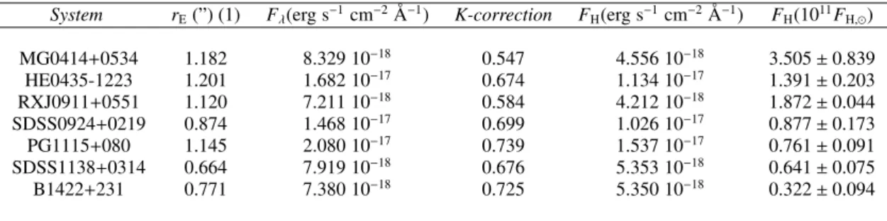
Table 3: Integrated flux within an aperture of radius rEbefore (Fλ) and after (FH) K-correction.
System rE(”) (1) Fλ(erg s−1cm−2Å−1) K-correction FH(erg s−1cm−2Å−1) FH(1011FH, )
MG0414+0534 1.182 8.329 10−18 0.547 4.556 10−18 3.505 ± 0.839 HE0435-1223 1.201 1.682 10−17 0.674 1.134 10−17 1.391 ± 0.203 RXJ0911+0551 1.120 7.211 10−18 0.584 4.212 10−18 1.872 ± 0.044 SDSS0924+0219 0.874 1.468 10−17 0.699 1.026 10−17 0.877 ± 0.173 PG1115+080 1.145 2.080 10−17 0.739 1.537 10−17 0.761 ± 0.091 SDSS1138+0314 0.664 7.919 10−18 0.676 5.353 10−18 0.641 ± 0.075 B1422+231 0.771 7.380 10−18 0.725 5.350 10−18 0.322 ± 0.094
References. (1) Sluse et al. (2012).
on each of these systematics values among all the data frames of each system, then conduct the shape parameters measurement again with the values shifted by an offset of the same magnitude as their error bar, one at a time. In this section, we focus on the new source of systematic errors, that is the subtraction of the arc. We used a similar approach that is based on building a 1σ error image of the arc and then measuring the shape param-eters after subtracting the sum of the arc image and its 1σ image. Each pixel of the data frame is affected by an uncertainty on its intensity, that is an output of the HST-NICMOS pipeline data reduction.2 We analytically compute the propagation of these uncertainties at each step of the arc reconstruction: the stacking and collapsing of traces within each sector, the fitting of a de Vaucouleurs law with the residuals symmetry criterion, the linear combination between this fit and arc datapoints, the re-scaling on individual traces, and the 2-D reconstruction of the arc. This yields a 1σ pixel map for the arc. To evaluate the error from the arc subtraction on the measurement of reff, for example, we conduct it twice, once after a subtraction of the correct arc image, and once deliberately subtracting too 2 Or that can be inferred from the data quality map and the photon
noise.
much arc, adding the 1σ value for each pixel in the arc image. The magnitudes of these error bars on reff, as well as for each systematic error source, are listed in Table 4. We find that the arc subtraction did not cause any noticeable error on the measurement of the PA nor of ε. Therefore, we do not update those parameters’ error calculations since B16 and their error budget can be found in the B16 CDS table (Biernaux et al. 2015).
4.2. On the integrated luminosity
We adopt a similar procedure to compute an error bar on FH. We consider the same sources of systematic errors (sky subtraction, point sources positions and intensities, and arc subtraction), con-duct the FHmeasurement with their values shifted by an offset equal to their 1σ error bar, and get their contribution to the total FHerror budget. On top of that, we take into account the effect from a miscalculation of reff on the FHmeasurement. Indeed, if reffis overestimated, for example, the central intensity I0would be underestimated and thus give a wrong result for the integrated flux. To quantify this effect, we conduct the FH measurement (from the I0determination) with a set of parameters that include an overestimate value of reff+σreff. Because we already compute
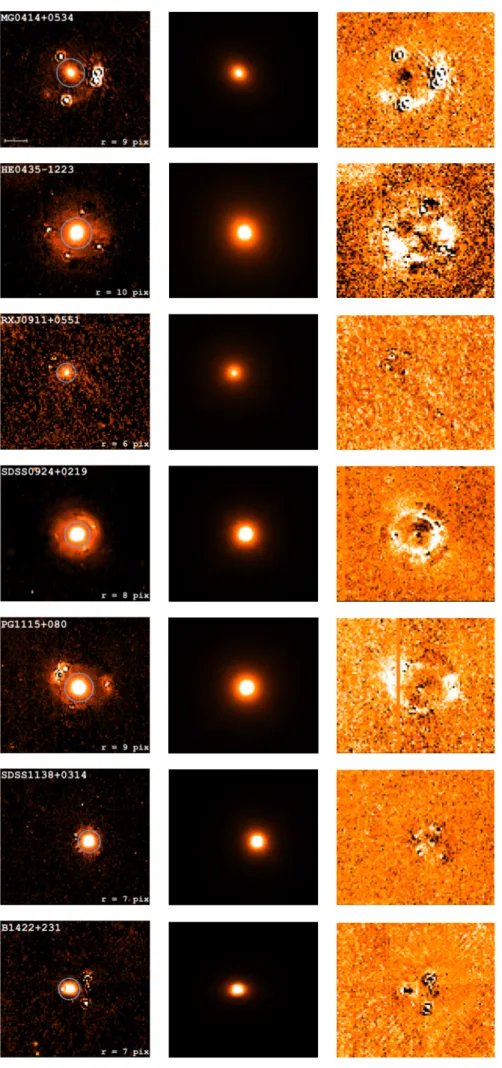
Fig. 5: Left to right: data frame after arc and point-source subtraction, best model and residuals for each system. The circle depicts the region of interest for the measurement of reff. The residual maps correspond to a ±3σ scale, white corresponding to > 3σ and black, < 3σ. Only one data
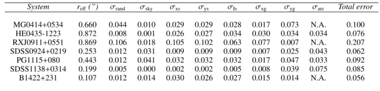
Table 4: Error budget on reff. From left to right: dispersion, sky subtraction, positions and intensities of the sources, position of the galactic centre, and subtraction of the arc. N.A. stands for "not applicable".
System reff(”) σrand σsky σxs σys σIs σxg σyg σarc Total error
MG0414+0534 0.660 0.044 0.010 0.029 0.029 0.028 0.017 0.073 N.A. 0.100 HE0435-1223 0.872 0.008 0.001 0.026 0.027 0.034 0.030 0.034 0.034 0.076 RXJ0911+0551 0.869 0.106 0.018 0.105 0.102 0.063 0.077 0.007 N.A. 0.207 SDSS0924+0219 0.253 0.012 0.031 0.009 0.009 0.009 0.007 0.025 0.043 0.062 PG1115+080 0.443 0.012 0.041 0.032 0.032 0.032 0.017 0.047 0.033 0.092 SDSS1138+0314 0.199 0.005 0.000 0.002 0.002 0.005 0.008 0.039 0.075 0.085 B1422+231 0.107 0.012 0.014 0.030 0.026 0.027 0.015 0.014 N.A. 0.056
an error bar on FH from the point source positions and inten-sities and from the sky subtraction, the σreff value we use here
only results from the combination of its dispersion and its error bar from the galaxy centre position (σrand, σxgand σyg). We find that while I0and reff are tightly correlated, the errors on the PA and ε did not influence the FHmeasurement. The error budget of FHis given in Table 5.
5. Results and discussion
The results of the half-light radii measurements are presented in Table 2 and compared to the B16 results. The new reff are on average 11 ± 6 % smaller than the B16 values, but their error bars overlap, except for SDSS1138+0314. This decrease can be expected as we subtract the contribution of the arc that leads to a positive bias on reff. Thanks to the subtraction of the arc, more datapoints can be taken into account for the reff measurement; we can consider a portion of the galaxy with a radius that is one or two pixels, or 17% on average, larger than before. Although this may seem like a small increase, it is of considerable importance because the reff value is highly sensitive to the wings of the de Vaucouleurs profile. Moreover, because the convolution mostly affects the central regions of the galaxy, we choose to ignore the first couple of pixels from the centre out, hence the interest in reaching as far out from the galactic centre as possible. The reff values obtained for the systems where no arc was subtracted have also changed, because of the new LRM. Changing the validity criterion in the LRM from only the slope of the model to the χ2 takes into account the individual uncertainties of the datapoints, granting less importance to the outliers and giving a more trustworthy reffvalue. Both these changes with regards to B16 constitute an improvement of the reffvalues.
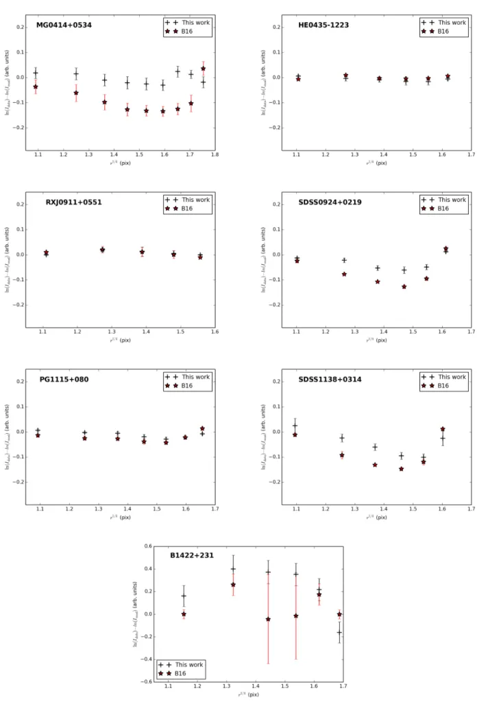
In B16, we performed a visual test to assess how well the de Vaucouleurs model represents the physical luminosity profiles of our lenses. The best model of each galaxy (the one appearing in Fig. 5) was convolved by the NIC2 PSF; its logarithmic radial profile ln I vs r1/4 was computed and subtracted from that of the data. If any residual curvature remained, it would mean that n , 4, n being the Sérsic index. We arrived at the conclusion that in four out of seven cases, the systems displayed a significant upwards curvature, indicating that their Sérsic index n may be higher than four. After the arc subtraction and the change in the LRM, we re-conducted this test to see if it changed our previous conclusion. As can be seen in Fig 6, for cases where there was no curvature in B16 (HE0435-1223 and RXJ0911+0551), the results remains unchanged. On the other hand, for the four cases (MG0414+0534, SDSS0924+0219, SDSS1138+0314, and PG1115+080) where we saw a significant upwards curvature
in B16, the test now shows less or no curvature at all. The result is particularly visible for MG0414+0534, where no arc subtraction was performed. This not only provides validation to the de Vaucouleurs model hypothesis, but also to the new LRM validity criterion. B1422+231 goes from an inconclusive result to displaying a downwards curvature. However, on its data frames, one of the point sources appears close in projection to the galaxy. Therefore, separating signal from that point source and from the lens is highly uncertain. We address that problem by applying a weighting mask to B1422+231 with null weights for the ill pixels. However, in spite of that treatment, some artefacts from the sources subtraction may remain on the B1422+231 data frames. As can be seen in Tables 4 and 5, the uncertainties coming from the positions and intensities of the sources are high for that system, and it has particularly large relative error bars. We therefore consider it less conclusive regarding the de Vaucouleurs profile test than the other systems.
By taking into account only one reasonable hypothesis (that the arc light distribution is radially symmetric), we can compute a more secure measurement of reff. However, the arc subtraction comes with a few drawbacks: first, it may produce some residual noise or artefacts on individual pixels values. We take that into account by computing the error maps of the reconstructed arc image and by including it in the reff error bars. The main weakness of this arc subtraction process is that it requires a lot of human intervention at each step, mostly for verification purposes, and is therefore very time-consuming. Since each system presents a different arc, each one with its own specificities linked to its position, the point sources positions and the configuration of the system, building a quicker, more automated version of the arc subtraction may lead to the loss of some precision.
The results of the FHmeasurement are given in Table 3, with their error bars and K-corrections. Since the rE values depend very little on the lens modelling, and since our work includes careful error processing, FH can be considered quite a robust estimate of the luminous flux in each lens. Together with the half-light radius measurement, these results make it possible to scale the distribution of ordinary matter in the lensing galaxies. Because lens modelling provides straightforward access to the total mass profile, this study could be the basis of a study of dark matter distribution in the lenses from our sample. We are currently addressing that question and the results are to be published in a future paper.
Fig. 6: Plots of the residual curvature when the ln I vs r1/4radial profile of the convolved best de Vaucouleurs model has been subtracted from that
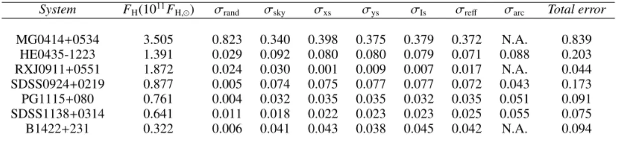
Table 5: Error budget on FH. From left to right: dispersion, sky subtraction, positions and intensities of the sources, measurement of reff, and
subtraction of the arc. N.A. stands for "not applicable".
System FH(1011FH, ) σrand σsky σxs σys σIs σreff σarc Total error
MG0414+0534 3.505 0.823 0.340 0.398 0.375 0.379 0.372 N.A. 0.839 HE0435-1223 1.391 0.029 0.092 0.080 0.080 0.079 0.071 0.088 0.203 RXJ0911+0551 1.872 0.024 0.030 0.001 0.009 0.007 0.017 N.A. 0.044 SDSS0924+0219 0.877 0.005 0.074 0.075 0.077 0.077 0.072 0.043 0.173 PG1115+080 0.761 0.004 0.032 0.035 0.035 0.032 0.035 0.051 0.091 SDSS1138+0314 0.641 0.011 0.018 0.022 0.023 0.023 0.025 0.055 0.075 B1422+231 0.322 0.006 0.041 0.043 0.038 0.045 0.042 N.A. 0.094 6. Conclusions
We completed the work from B16 by adding the arc subtraction and improving the LRM. We obtained more secure measure-ments for reff. Although the arc subtraction is time-consuming and requires human intervention at many steps, not taking the arc into account leads to an overestimate of reff of about 11% in the case of our sample. We performed a highly detailed er-ror calculation and obtained safe erer-ror bars for reff and FH. We have also verified that the de Vaucouleurs profile satisfactorily represents the physical light distribution of our sample elliptical galaxies. Eventually, our study yielded a high-quality characteri-sation of the quantity of luminous matter (FH) in the lenses from this sample. We intend to use these results to conduct a study of dark matter distribution in early-type galaxies, thus contributing to major debates in galaxy evolution and cosmology.
Acknowledgements. J. Biernaux acknowledges the support of the F.R.I.A. fund of the F.N.R.S. The authors are thankful to Dominique Sluse for his kind and valuable help.
References
Bertin, G., Bertola, F., Buson, L. M., et al. 1994, A&A, 292, 381
Biernaux, J., Magain, P., Sluse, D., & Chantry, V. 2015, VizieR Online Data Catalog, 358
Biernaux, J., Magain, P., Sluse, D., & Chantry, V. 2016, A&A, 585, A84 Cappellari, M., Romanowsky, A. J., Brodie, J. P., et al. 2015, ApJ, 804, L21 Chantry, V. & Magain, P. 2007, A&A, 470, 467
Chantry, V., Sluse, D., & Magain, P. 2010, A&A, 522, A95 Colina, L., Bohlin, R. C., & Castelli, F. 1996, AJ, 112, 307 Courbin, F., Chantry, V., Revaz, Y., et al. 2011, A&A, 536, A53 Dekel, A., Stoehr, F., Mamon, G. A., et al. 2005, Nature, 437, 707 Fioc, M. & Rocca-Volmerange, B. 1997, A&A, 326, 950
Hook, R. & Krist, J. 1997, Space Telescope European Coordinating Facility Newsletter, 24, 10
Krist, J. E. & Hook, R. N. 1997, in The 1997 HST Calibration Workshop with a New Generation of Instruments, ed. S. Casertano, R. Jedrzejewski, T. Keyes, & M. Stevens, 192
Lewis, A. 2008, Phys. Rev. D, 78, 023002
Magain, P., Courbin, F., & Sohy, S. 1998, ApJ, 494, 472
Muñoz, J. A., Falco, E. E., Kochanek, C. S., et al. 1998, Ap&SS, 263, 51 Peng, C. Y., Ho, L. C., Impey, C. D., & Rix, H.-W. 2002, AJ, 124, 266 Peng, C. Y., Ho, L. C., Impey, C. D., & Rix, H.-W. 2010, AJ, 139, 2097 Romanowsky, A. J., Douglas, N. G., Arnaboldi, M., et al. 2003, Science, 301,
1696
Sluse, D., Chantry, V., Magain, P., Courbin, F., & Meylan, G. 2012, A&A, 538, A99