Discovery of the atomic iron tail of comet McNaught using the Heliospheric Imager on STEREO

L93

The Astrophysical Journal, 661: L93–L96, 2007 May 20 䉷 2007. The American Astronomical Society. All rights reserved. Printed in U.S.A.

DISCOVERY OF THE ATOMIC IRON TAIL OF COMET McNAUGHT USING THE HELIOSPHERIC IMAGER ON STEREO

M. Fulle

INAF–Osservatorio Astronomico Via Tiepolo 11, I-34143 Trieste, Italy; fulle@oats.inaf.it

F. Leblanc1

Service d’Aeronomie du CNRS/IPSL, 91371 Verrieres le Buisson, France

R. A. Harrison, C. J. Davis, and C. J. Eyles2 Rutherford Appleton Laboratory, Oxfordshire, UK

J. P. Halain

Centre Spatial de Liege, Belgium

R. A. Howard

Naval Research Laboratory, Washington, DC

D. Bockele´e-Morvan

Observatoire de Paris–Meudon, 5 Place Jules Janssen, 92195 Meudon, France

G. Cremonese

INAF–Osservatorio Astronomico, Padova, Italy

and T. Scarmato

UAI-CARA, San Costantino di Briatico (VV), Italy

Received 2007 March 22; accepted 2007 April 6; published 2007 April 27

ABSTRACT

In 2007 January, at the heliocentric distancer!0.3AU, comet McNaught 2006P1 became the brightest comet since C/Ikeya-Seki 1965S1 and was continuously monitored by space-based solar observatories. We provide strong evidence that an archlike tail observed by the Heliospheric Imager aboard the STEREO spacecraft is the first ever detected tail composed of neutral Fe atoms. We obtain an Fe lifetime 4 s at

t p (4.1Ⳳ 0.4) # 10

AU, in agreement with theoretical predictions of the photoionization lifetime. The expected dust

tem-r p 0.25

perature is inconsistent with iron sublimation, suggesting that Fe atoms are coming from troilite evaporation.

Subject headings: atomic data — comets: general — comets: individual (McNaught 2006P1)

1.INTRODUCTION

Comets provide unique information on the cosmic abun-dances of the solar nebula, which collapsed to form the solar system. Very few data regard the metallic content of comet nuclei, because the temperatures at which metals sublimate are experienced by rare Sun-grazing comets, usually too close to the Sun to be observed by ground-based spectroscopes. In par-ticular, iron was remotely detected in spectra of comet Ikeya-Seki 1965S1 only (Preston 1967). Laboratory analyses of sam-ples collected at comet 81P/Wild 2 showed that most iron is in the form of troilite (FeS) grains (Zolensky et al. 2006). Is this true for all comets? Can we use space-solar observatories to detect iron in Sun-grazing comets and to extract Fe physical properties? This report tries to answer these questions. Since Mercury’s surface temperature is close to that of the dust ejected from comet McNaught at perihelion, our results may address exosphere observations of future space missions such as MESSENGER (launched on 2004) and BepiColombo (to be launched on 2013).

2.OBSERVATIONS

Launched in 2006 October, the NASA STEREO mission is designed to make three-dimensional observations of the Sun and its outer atmosphere, the heliosphere (Harrison et al. 2005).

1_{Current address: INAF–Osservatorio Astronomico, Via Tiepolo 11,} I-34143 Trieste, Italy.

2_{Current address: University of Birmingham, UK.}

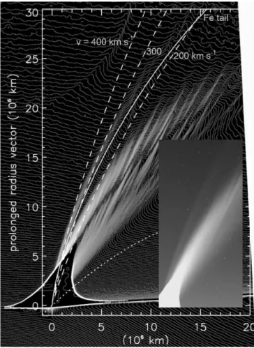
The mission comprises two spacecraft placed into heliocentric orbits, one moving ahead of the Earth and one behind. These two spacecraft (named Ahead and Behind and referred to as A and B, respectively) move away from the Earth at a rate that increases the Earth-Sun-spacecraft angle by 22.5⬚ each year. While most of the telescopes on board each spacecraft are Sun-pointing, one instrument on each spacecraft—the Heliospheric Imager (HI)—is mounted on the side of the spacecraft and looks back at the Sun-Earth line, its aim being to detect and study Earth-directed solar-ejected clouds known as coronal mass ejections (CMEs). Each instrument comprises two wide-field visible light cameras called HI-1 and HI-2. HI-1 has a passband between 630 and 730 nm and has a 20⬚ field of view centered 13.65⬚ from the Sun center. The HI-2 camera has a 400–1000 nm passband and has a 70⬚ field of view centered 53.35⬚ from the Sun center. While the primary science goal of these instruments is to detect Earth-impacting CMEs, it was anticipated that data from these wide-field cameras would be useful for many other science applications, including the obser-vation of comets (Davis & Harrison 2005). During the perihelion passage of comet McNaught, occurring on 2007 January 12.8 UT at the heliocentric distancer p 0.171 AU (corresponding to_{2.56 # 10}7km), the HI-1 instrument on the B spacecraft (HI-1B) took the best resolved images (Nemiroff & Bonnell 2007) of the dust tail with many striae (probably due to fragmentation of fluffy grains) and, well separated from the main dust tail, of an archlike tail stretching_{3 # 10}7 km (Fig. 1).

L94 FULLE ET AL. Vol. 661

Fig. 1.—Image (insert at the same scale and orientation) and isophotes of the

tails of comet McNaught 2006P1 on 2007 January 12.5 UT taken by HI-1B (scale in 106_{km units). The coma around the nucleus has saturated the CCD.} The archlike tail corresponds to the solid white line that follows the crest of the isophotes on the left of the main dust tail. The circular arc in the upper left-hand corner is an artifact. Three striae from the dust tail overlap the archlike tail. The (0, 0) point corresponds to the comet nucleus position computed in a STEREO-centric reference frame and was identified thanks to stars visible in the original images (see the insert). All the following lines are projected on the sky in a

STEREO-centric reference frame. Vertical axis: Antisolar direction (the Sun is

exactly in the bottom direction at 2.56 # 107_{km from the nucleus). Dotted line:} Comet’s orbit. Dashed lines: Model ion tails moving at the given solar wind velocity. Solid line: Theoretical Fe tail. The apparent shift to the right of the fitting line closer than 107_{km from the nucleus is due to the brightness gradient} of the main dust tail.

3.MODELS OF THE ARCHLIKE TAIL

A first possibility is that the archlike tail is an ion tail. The coma releases ions along the comet’s orbit, which are then dragged by the solar wind. Figure 1 displays the tail axis of ions trapped in a solar wind with velocity of 200, 300, or 400 km s⫺1. A velocity of 400 km s⫺1provides the best fit of the archlike tail at 5 # 106

km from the nucleus, whereas at 3 # 107_{km from the nucleus, the best fit is given by a velocity of} 200 km s⫺1. These velocities would imply that the solar wind accelerated from 200 km s⫺1 on January 10.8 to 400 km s⫺1 on January 12.5. However, this possibility is inconsistent with the archlike tail observed on January 13.5 (Fig. 2), which would require the acceleration from 250 km s⫺1on January 12.5 to 400 km s⫺1 on January 13.5, and with data from the NASA

Advanced Composition Explorer (Stone et al. 1990), which

observed a roughly constant velocity of the solar wind of 360 km s⫺1 between January 12.5 and 15.5, and of 600 km s⫺1 between January 15.5 and 20.0. The huge water production rate suggested by the HCN loss rate (N. Biver 2007, private

communication) implies such a wide diamagnetic cavity that water ions (the only ones known to have emission lines between 630 and 730 nm [Wyckoff 1982; Feldman et al. 2004]) should be photodissociated (Huebner et al. 1992) before being able to interact with the solar wind to form the C/2006P1 ion tail.

A second possibility is that the tail particles are driven by solar radiation pressure and gravity forces. The ratio between these forces is the r-independent b-parameter. If, along the

orbit, the nucleus ejects particles with a constant b-value, the

tail axis is perfectly fitted by lines named syndynes (Finson & Probstein 1968). The archlike tail is fitted by a syndyne of , which is too high for most dust compositions. Only pure

b≈ 6

graphite spheres with a radius of 80 nm may approach such a

b-value (Burns et al. 1979). In such a case, larger graphite

grains, less efficiently destroyed by sublimation, should be ob-served between the archlike and dust tails. On the other hand, submicron grains are much smaller than red light wavelengths, so that no strong scattering should occur in the HI-1B passband. At the end, such small grains are probably charged and dragged by the solar wind. Very porous dust aggregates may approach highb-values, and all observations point out that dust is

prob-ably fluffy in all comets. However, the fact that no comet ever showed a dust tail withb11 (Fulle 2004) suggests that fluffy grains also have low b-values. Computations of b for such

aggregates are not yet available (Kolokolova et al. 2004). A tail composed of neutral atoms pushed away by solar radiation pressure (Fulle 2004) is actually more consistent with the observations. A neutral Na tail was observed in comet Hale-Bopp 1995O1 (Cremonese et al. 1997), but the computed Na tail is close to a syndyne ofb≈ 80and does not fit the archlike tail. Theb-value of neutral atoms depends on the solar radiation

pressure, which is proportional to the total number of excitations per unit time of an atom, the g-factor (Fulle 2004; Cremonese et al. 1997). We have computedb as a function of the heliocentric

radial velocity for the 13 most abundant chemical species using the solar UV flux (Huebner et al. 1992), the high-resolution visible solar flux (Kurucz et al. 1984)—both in quiet-Sun con-ditions—and oscillator strengths for all resonant lines (Morton 2003, 2004). For each element, we have calculated the atomic tail using the velocity-dependentb, which has then been fitted

by syndynes providing us with a range of equivalent constant

b-values consistent with each atomic tail. Table 1 shows that

only Al and Fe have an equivalent constantb≈ 6. Although Fe resonant lines have wavelengths between 194 and 525 nm, Fe has many spectral lines associated with transitions from upper to lower excited states between 630 and 730 nm (Beristain et al. 1998). Neutral Fe emission lines were the strongest in the spectra of comet Ikeya-Seki 1965S1 observed atr p 0.14AU (Preston 1967).

We have computed the motion of Fe atoms according to the Fe velocity-dependent b. The theoretical Fe tail matches very

well the archlike tail as indicated Figure 1. While the comet exited the HI-1B field of view a few hours after perihelion, HI-1A observed the comet between January 12.0 and 14.5. For each of these observations, the projection on the sky of the Fe tail was calculated following the same numerical approach. The neutral Fe tail fits all available observations as illustrated by Figure 2. In order to derive the surface brightness along the axis of the archlike tail, we have considered sections of the image oriented perpendicular to the tail axis. These sections are dominated by the dust tail background, fitted by Gaussians with parameters calculated for each slice. The dust tail Gaus-sians overlap a background due to the solar corona and the view-angle–dependent sensitivity, which, close to the archlike

No. 1, 2007 IRON TAIL OF COMET McNAUGHT L95

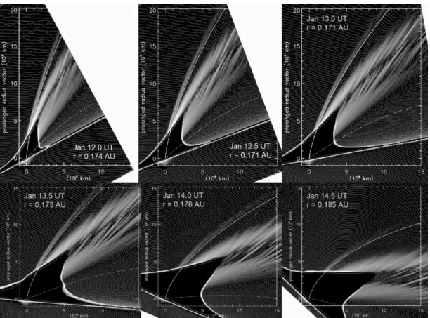
Fig. 2.—Fit of the archlike tail by means of the computed Fe tail (solid white lines) for six HI-1A comet observations. The edge of the field of view is visible

in the first two top panels (January 12.0 and 12.5; the comet just entered the field of view) and in the last two bottom panels (January 14.0 and 14.5; the comet nucleus is exiting the field of view). The images are dominated by the dust tail with many striae; some of them overlap the archlike tail. The vertical axis is along the antisolar direction. The Sun-comet distance r is also given; the perihelion occurred between the second and third panels. See Fig. 1 for further explanations.

TABLE 1

Computed Equivalent Constantb and Photoionization Lifetimes

Atom Equivalentb

Photoionization Lifetime (s) at 1 AU

Huebner et al. (1992) This Letter H . . . 0.20Ⳳ 0.15 1.4 # 107 _{7.8 # 10}6 C . . . (1.15Ⳳ 0.05) # 10⫺3 2.4 # 106 _{1.1 # 10}6 N . . . (5Ⳳ 1) # 10⫺5 5.4 # 106 _{2.0 # 10}6 O . . . (4Ⳳ 2) # 10⫺5 4.7 # 106 2.0 # 106 Na . . . 75Ⳳ 5 6.2 # 104 _{1.9 # 10}5 Mg . . . 1.3Ⳳ 0.3 … 2.1 # 106 Al . . . 5Ⳳ 2 … 1.4 # 103 Si . . . (7Ⳳ 1) # 10⫺2 … 4.4 # 104 S . . . (6Ⳳ 1) # 10⫺4 9.4 # 105 _{4.2 # 10}5 Ar . . . (4Ⳳ 1) # 10⫺8 3.3 # 106 _{1.4 # 10}6 K . . . 56Ⳳ 2 4.3 # 104 _… Ca . . . 40Ⳳ 10 … 1.4 # 104 Fe . . . 6.0Ⳳ 0.5 … 5.1 # 105 tail, is well fitted by a linear gradient calculated for each slice. We subtract both Gaussian and linear backgrounds of each slice, getting sections with emissions from only the archlike tail, which provide us the tail brightness and width (Fig. 3). A definitive calibration of the cameras can only be carried out after many weeks of observations. For a preliminary calibra-tion, in the HI-1A image taken on January 14.0 UT, we have found four Hipparcos stars of spectrum G0 V–G5 V of V magnitude betweenV p 6.11 andV p 8.55. The HI-1 pass-band is well approximated by the w passpass-band (Tedesco et al. 1982), with zero color indexV⫺ wfor solar-type stars, pro-viding a zero-point magnitudeV p 19.280 Ⳳ 0.13.

4.RESULTS AND CONCLUSIONS

The tail brightness plotted in Figure 3 can be fitted according to dust tail theory (Fulle 2004). The observed brightness de-creases by orders of magnitude faster than that expected for a dust tail. This is strong evidence against the dust (graphite or fluffy grains) tail hypothesis. Support for the iron tail is in fact obtained by fitting the observed tail brightness with the theory of the neutral atom tail (Fulle 2004; Cremonese et al. 1997), which accounts for a lifetimet against ionization. All archlike

tail profiles observed between January 12.0 and 14.5 are best fitted by the same ionization lifetime 4s

t p (4.1Ⳳ 0.4) # 10

at the averaged tailr≈ 0.25AU (Fig. 3). This fact confirms that the image background was correctly subtracted from the data and suggests that the Fe loss rate remained roughly constant at

AU. Since t depends on 2, we get

r≤ 0.2 r t p (6.6Ⳳ

s at AU. Table 1 provides the lifetimes against 5

0.6) # 10 r p 1

photoionization of the most abundant chemical species calculated using the same solar flux as before and theoretical cross sections (Verner et al. 1996). Taking into account the uncertainty on the solar EUV-UV flux and on the photoionization cross sections, the Fe photo-ionization lifetime matches very well the observed

t-value, whereas the Al lifetime is a factor 400 shorter. Our Na

lifetime computation agrees with 5 s observed at

t p 1.7 # 10

1 AU (Cremonese et al. 1997). When we assume a zero spectral index, the Fe tail brightness becomes10⫺8dJy sr⫺1(whered is

the Fe atom column density; Fig. 3), so that our preliminary calibration suggests an Fe loss rate_{Q ≈ 10 s ≈ 10 Q}30 ⫺1 ⫺1

Fe H O2

of C/1995O1 at perihelion (Bockele´e-Morvan et al. 2004). When we assume the dust-to-gas ratio x≈ 10 observed in 1P/Halley (Fulle 2004), sinceAfrof C/2006P1 is a factor 10 higher than

L96 FULLE ET AL. Vol. 661

Fig. 3.—Measured surface brightness along the tail axis (diamonds: HI-1B

data of January 12.5 UT; triangles: HI-1A data of January 14.0 UT) and fit (solid line) by means of the theoretical brightness of a neutral Fe tail with a lifetime_{t p 4.1 # 10}4s. Measured tail FWHM (mult crosses: January 12.5, HI-1B; plus signs: January 14.0, HI-1A) and fit (dashed line) by means of an Fe expansion velocity of 1.5 km s⫺1. The symbol sizes give the measurement standard deviation. No tail brightness or width measurements are possible at nucleus distances smaller than 4 # 106_{km, owing to image saturation, and} larger than 1.5 # 107_{km, due to pollution from dust striae. In such a range,} the terminal Fe heliocentric radial velocity increases from 80 to 120 km s⫺1_. Preliminary calibration suggests that the unit relative tail brightness corre-sponds to 106_{Jy sr}⫺1_{and to the Fe atom column density} 14_m⫺2_.

d p 10

that of C/1995O1 at perihelion (Sostero 2007), we get QFe≈ (or even less if ), in agreement with Fe

abun-⫺3

10 Qdust x110

dance in comet dust samples (Zolensky et al. 2006).

The tail width provides the ejection velocity of the Fe atoms from the coma, which results in1.5Ⳳ 0.2km s⫺1, in agreement with available HCN velocity-resolved spectra (Biver 2007, pri-vate communication) and fluid-dynamic coma models at r≤ AU (Crifo et al. 2004). Fe atoms may be released from the 0.2

nucleus surface and/or from dust, and then accelerated to the gas velocity in the large collisional coma. Fe atoms may sub-limate from fluffy troilite grains (Zolensky et al. 2006), sug-gesting a dust temperatureT1680 K (FeS condensation tem-perature [Pollack et al. 1994]) atr≤ 0.2AU, in agreement with blackbody extrapolations of the dust temperature observed at comet 1P/Halley (Tokunaga et al. 1988). All data on dust tem-perature (Kolokolova et al. 2004) are inconsistent with direct sublimation of metallic Fe, which would requireT11000 K (Knacke et al. 1991) atr≤ 0.2 AU. Troilite may be the most abundant sulfide not only in comets. Mercury’s crust could have a composition similar to the mineral assemblages found in aubritic meteorites (Burbine et al. 2002), with troilite the most abundant sulfide, usually found in abundance ranging from 1% volume to 7% volume of Shallowater aubrite. The bright radar spots seen at Mercury’s poles may be due to vol-ume scattering from elemental sulfur (Sprague et al. 1995), present in the regolith as iron sulfides.

We acknowledge the careful review of the first draft by Bruno Caprile and John Danziger.

REFERENCES Beristain, G., Edwards, S., & Kwan, J. 1998, ApJ, 499, 828

Bockele´e-Morvan, D., Crovisier, J., Mumma, M. J., & Weaver, H. A. 2004, in Comets II, ed. M. C. Festou, H. U. Keller, & H. A. Weaver (Tucson: Univ. Arizona Press), 391

Burbine, T. H., McCoy, T. J., Nittler, L. R., Benedix, G. K., Cloutis, E. A., & Dickinson, T. L. 2002, Meteoritics Planet. Sci., 37, 1233

Burns, J. A., Lamy, P. L., & Soter, S. 1979, Icarus, 40, 1 Cremonese, G., et al. 1997, ApJ, 490, L199

Crifo, J. F., Fulle, M., Komle, N. I., & Szego, K. 2004, in Comets II, ed. M. C. Festou, H. U. Keller, & H. A. Weaver (Tucson: Univ. Arizona Press), 471

Davis, C. J., & Harrison, R. A. 2005, Adv. Space Res., 36, 1524

Feldman, P. D., Cochran, A. L., & Combi, M. R. 2004, in Comets II, ed. M. C. Festou, H. U. Keller, & H. A. Weaver (Tucson: Univ. Arizona Press), 425

Finson, M. L., & Probstein, R. F. 1968, ApJ, 154, 327

Fulle, M. 2004, in Comets II, ed. M. C. Festou, H. U. Keller, & H. A. Weaver (Tucson: Univ. Arizona Press), 565

Harrison, R. A., Davis, C. J., & Eyles, C. J. 2005, Adv. Space Res., 36, 1512 Huebner, W. F., Keady, J. J., & Lyon, S. P. 1992, Ap&SS, 195, 1

Knacke, O., Kubaschewski, O., & Hesselmann, K. 1991, Thermochemical Properties of Inorganics Substances (New York: Springer)

Kolokolova, L., Hanner, M. S., Levasseur-Regourd, A. C., & Gustafson, B. A. S. 2004, in Comets II, ed. M. C. Festou, H. U. Keller, & H. A. Weaver (Tucson: Univ. Arizona Press), 577

Kurucz, R. L., Furenlid, I., Brault, J., & Testerman, L. 1984, Solar Flux Atlas from 296 to 1300 nm (National Solar Observatory Atlas, No. 1) (Sunspot: NSO)

Morton, D. C. 2003, ApJS, 149, 205 ———. 2004, ApJS, 151, 403

Nemiroff, R., & Bonnell, J. 2007, Astronomy Picture of the Day, http:// antwrp.gsfc.nasa.gov/apod/ap070117.html

Pollack, J. B., Hollenbach, D., Beckwith, S., Simonelli, D. P., Roush, T., & Fong, W. 1994, ApJ, 421, 615

Preston, G. W. 1967, ApJ, 147, 718

Sostero, G. 2007, Cometary Data Archive for Amateur Astronomers, http:// cara.uai.it

Sprague, H. A. L., Hunten, D. M., & Lodders, K. 1995, Icarus, 118, 211 Stone, E. C., et al. 1990, in AIP Conf. Proc. 203, Particle Astrophysics: The

NASA Cosmic Ray Program for the 1990s and Beyond, ed. M. V. Jones, F. J. Kerr, & J. F. Ormes (New York: AIP), 48

Tedesco, E. F., Tholen, D. J., & Zellner, B. 1982, AJ, 87, 1585

Tokunaga, A., Golish, T., Griep, D., Kaminski, C., & Hanner, M. S. 1988, AJ, 96, 1971

Verner, D. A., Ferland, G. J., Korista, K. T., & Yakovlev, D. G. 1996, ApJ, 465, 487

Wyckoff, S. 1982, in Comets, ed. L. L. Wilkening (Tucson: Univ. Arizona Press), 3