Densités de Copules Archimédiennes Hiérarchiques
par
David-Olivier Pham
Département de Mathématiques Faculté des arts et des sciences
Mémoire présenté à la Faculté des études supérieures en vue de l’obtention du grade de Maître ès sciences (M.Sc.)
en mathématiques orientées en actuariat
Avril, 2012
c
Ce mémoire intitulé:
Densités de Copules Archimédiennes Hiérarchiques
présenté par: David-Olivier Pham
a été évalué par un jury composé des personnes suivantes: Bédard Mylène, président-rapporteur
Morales Manuel, directeur de recherche Doray Louis, membre du jury
Nested Archimedean copulas recently gained interest since they generalize the well-known class of Archimedean copulas to allow for partial asymmetry. Sampling algorithms and strategies have been well investigated for nested Archimedean copulas. However, for likelihood based inference such as estimation or goodness-of-fit testing it is important to have the density. The present work fills this gap. After a short introduction on copula and nested Archimedean copulas, a general formula for the derivatives of the nodes and inner generators appearing in nested Archimedean copulas is developed. This leads to a tractable formula for the density of nested Archimedean copulas. Various examples including famous Archimedean families and transformations of such are given. Further-more, a numerically efficient way to evaluate the log-density is presented.
RÉSUMÉ
Les copulas archimédiennes hiérarchiques ont récemment gagné en intérêt puisqu’elles généralisent la famille de copules archimédiennes, car elles introduisent une asymétrie par-tielle. Des algorithmes d’échantillonnages et des méthodes ont largement été développés pour de telles copules. Néanmoins, concernant l’estimation par maximum de vraisem-blance et les tests d’adéquations, il est important d’avoir à disposition la densité de ces variables aléatoires. Ce travail remplie ce manque. Après une courte introduc-tion aux copules et aux copules archimédiennes hiérarchiques, une équaintroduc-tion générale sur les dérivées des noeuds et générateurs internes apparaissant dans la densité des copules archimédiennes hiérarchique. sera dérivée. Il en suit une formule tractable pour la densité des copules archimédiennes hiérarchiques. Des exemples incluant les familles archimé-diennes usuelles ainsi que leur transformations sont présentés. De plus, une méthode numérique efficiente pour évaluer le logarithme des densités est présentée.
Keywords: Nested Archimedean copulas, generator derivatives, likelihood-based in-ference.
ABSTRACT . . . . v CONTENTS . . . vii LIST OF TABLES . . . ix LIST OF FIGURES . . . xi ACKNOWLEDGMENTS . . . xiii CHAPTER 1: COPULAS . . . . 1 1.1 Preliminaries . . . 1
1.2 Definitions and Basic Properties of Copulas . . . 2
1.3 Sklar’s Theorem . . . 4
1.4 Random Vectors and Copulas . . . 5
1.5 Density and Conditional Distributions . . . 7
1.6 Symmetries of Copulas . . . 8
1.7 Dependence Measures . . . 9
CHAPTER 2: ARCHIMEDEAN AND NESTED ARCHIMEDEAN COP-ULAS . . . 11
2.1 Archimedean Copulas . . . 11
2.1.1 Bivariate Archimedean Copulas . . . 12
2.1.2 Multivariate Archimedean Copulas . . . 13
2.2 Nested Archimedean Copulas . . . 15
2.3 Parametric Archimedean Families . . . 19
CHAPTER 3: DENSITIES OF NESTED ARCHIMEDEAN COPULAS 25 3.1 Introduction . . . 25
3.2 Inner generator derivatives and densities for two-level nested Archimedean copulas . . . 26
3.2.1 The basic idea . . . 26
3.2.2 The tools needed: Faà di Bruno’s formula and Bell polynomials . . 27
3.2.3 The main result . . . 31
3.3 Example - Families and transformations . . . 33
3.3.1 Tilted outer power families, Clayton and Gumbel copulas . . . 33
3.3.2 Ali–Mikhail–Haq copulas . . . 35
3.3.3 Joe copula . . . 37
3.3.4 Frank Copula . . . 40
3.3.5 A nested Ali–Mikhail–Haq ¶ Clayton copula . . . 41
3.4 Numerical evaluation . . . 42
3.4.2 The -log-likelihood of two-parameter nested Clayton and Gumbel copulas . . . 44 3.5 Densities for three- (and higher-) level nested Archimedean copulas . . . . 45 CHAPTER 4: CONCLUSION . . . 55 BIBLIOGRAPHY . . . 57
2.I Generator and its dth derivaties of the Gumbel, Clayton, Ali-Mikail-Haq , Frank and Joe copulas. . . 19 2.II Inverse of the generator and its first derivative of the Gumbel,
Clay-ton, Ali-Mikail-Haq , Frank and Joe copula. . . 20 2.III Inner generator and the distribution F = LS≠1[Â] of the Gumbel,
2.1 Tree structure of a d-dimensional partially nested Archimedean cop-ula with qd0
s1=1ds1 = d. . . 16
2.2 Pairwise scatterplots of 250 simulated points from a four-dimensional hierarchical nested Archimedean copula C0{C1(u1, u2),C2(u3, u4)}
with Gumbel generators. ◊ = (◊0, ◊1, ◊2)Tcorresponds to Kendall’s
tau · = (·0, ·1, ·2)T= (0.3,0.5,0.7)T . . . 17
2.3 One thousand simulated points from the Gumbel and Clayton copula with parameter ◊ corresponding to a Kendall’s tau of 0.5. . . 22 2.4 One thousand simulated points from the Joe and Frank copula with
parameter ◊ corresponding to a Kendall’s tau of 0.5. . . 22 2.5 One thousand simulated points from the Ali-Mikhail-Haq Copula
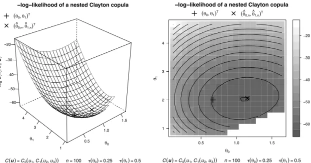
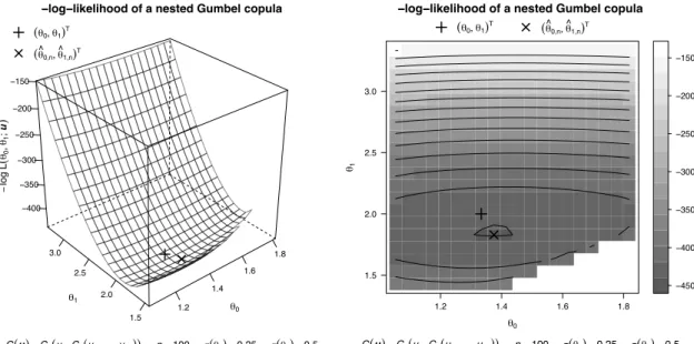
with parameter ◊ corresponding to a Kendall’s tau of 0.3 . . . 23 3.1 Wireframe (left) and level plot (right) of the -log-likelihood of a
three-dimensional nested Clayton copula C(u) = C0{u1, C1(u2, u3)} with
parameters ◊0= 2/3 (Kendall’s tau equals 0.25) and ◊1= 2 (Kendall’s
tau equals 0.5) based on a sample of size n = 100. . . 45 3.2 Wireframe (left) and level plot (right) of the -log-likelihood of a
ten-dimensional nested Clayton copula C(u) = C0{u1, C1(u2, . . . , u10)}
with parameters ◊0 = 2/3 (Kendall’s tau equals 0.25) and ◊1 = 2
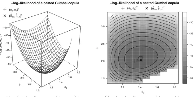
(Kendall’s tau equals 0.5) based on a sample of size n = 100. . . 46 3.3 Wireframe (left) and level plot (right) of the -log-likelihood of a
three-dimensional nested Gumbel copula C(u) = C0{u1, C1(u2, u3)} with
parameters ◊0= 4/3 (Kendall’s tau equals 0.25) and ◊1= 2 (Kendall’s
tau equals 0.5) based on a sample of size n = 100. . . 46 3.4 Wireframe (left) and level plot (right) of the -log-likelihood of a
ten-dimensional nested Gumbel copula C(u) = C0{u1, C1(u2, . . . , u10)}
with parameters ◊0 = 4/3 (Kendall’s tau equals 0.25) and ◊1 = 2
(Kendall’s tau equals 0.5) based on a sample of size n = 100. . . 47 3.5 Tree structure (some arguments are omitted) for a three-level nested
I would like to thank Johanna Neölehová and Christian Genest for having introduced me to the wonderful world of mathematical statistics and copulas. I am also indebted to Paul Embrechts, who accepted to supervise my master’s thesis, and to Manuel Morales, who provided me with a glimpse of the research environment in Montreal. This work could not have been done without the support, enthusiasm and expertise of Marius Hofert. He carefully presented me the problem, helped me throughout the writing of this thesis, and above all shared his experience and knowledge about copulas and his actual research results.
In recent years, there have been several critics about the uses of too sophisticated mathematical and statistical models, especially in finance. People do argue against the restrictive hypothesis of the celebrated Black-Scholes formula for option pricing, however, there also is a lot of concern about the use of copulas. Copulas are tools to describe stochastic dependencies, and during recent years, a certain class of copulas was used in the financial industries to price a large amount of financial derivatives. Indeed, Embrechts (2009) provided three reasons to explain the recent interest of copulas in research: finance, finance, finance. However, although there has been a large amount of evidences and cautions against the uses of this class of copulas, people still used it. It resulted in an inadequate pricing of financial products and finally contributed in a crash of the financial market, a worldwide recession and a large amount of loss for people who did not listen to the advices.
Since then, there have been discussions among academics and profesionals about using complex numerical models in the industries. However, it is undeniable that sophisticated statistical methods have their place there. Copulas, for instance, provide a useful and successful tool to understand and forecast multivariate random behaviors in hydrology, in medical and climate researches.
I am on the side of those who think that it can only be helpful to society to have at its disposition robust and well understood mathematical tools. This belief motivates the subject of this thesis. Hierarchical models using Archimedean copulas have recently gained interest in order to describe multidimensional phenomena, nevertheless, densities of such model are not known. This work tries to fill the gap.
Chapter 1 starts with a little introduction to copulas. Chapter 2 presents known results about (nested) Archimedean copulas and sets the framework for the next chapter. Chapter 3 is the core of this thesis. It begins by giving the general strategy and results from analysis to compute the densities of nested Archimedean copulas. Examples and numerical implementation are also covered. It is worth to underscore that numerical implementation of copulas in high dimension is a tremendously hard task. Fortunately, the R package nacopula helps a lot.
COPULAS
In this chapter, we present general results about copulas and multivariate stochastic dependencies and cover results needed for this work. For more details, the interested reader may consult the more detailed literature, for instance the excellent textbooks McNeil et al. (2005), Nelsen (2007) or the mathematically self-contained PhD thesis Hofert (2010).
1.1 Preliminaries
In the study of univariate random behavior, one can naturally ask the question, given the level p between zero and one, which observation q is needed so that P(X Æ q) = p, where X is a real-valued random variable. In the case where the distribution function is bijective, the answer is trivially given by the inverse function. However, when this is not the case, one has to pay attention to what is allowed during the computations and what happens when one uses this inverse. It leads us to the following definition, where R is the set of real number and I is the unit cube [0,1].
Definition 1.1 (Generalized Inverse). Let F : ¯R æ I be an increasing function with the convention that F (±Œ) is interpreted in the sense of the limit of F(x) as x tends to ±Œ. Then the generalized inverse F≠: I æ ¯R of F is defined by
F≠(y) = inf {x œ R : F(x) Ø y}
with the convention that inf ÿ = Œ.
Note that F≠(y) = ≠Œ if and only if F(x) Ø y for all x œ R and F≠(y) = Œ if and
only if F (x) < y for all x œ R. As stressed before, the generalized inverse must be ma-nipulated with care. The main properties are precisely stated in Embrechts and Hofert (2011). The following proposition gives a useful result.
Proposition 1.2. Let F : ¯R æ I be the distribution function of X. Then the inequality
F(x) Ø y stands if and only if x Ø F≠(y).
Proof
See Embrechts and Hofert (2011).
The following proposition is the key to sampling univariate random variables with distribution function F . It says that if one can sample the uniform distribution, sam-pling from F can theoretically be performed. It is known as the inversion method.
Proposition 1.3. Let X be an univariate random variable following the distribution function F . If U ≥ U[0,1], then F≠(U) ≥ F. Moreover, if F is continuous, then F(X) ≥
U[0,1]. Proof
By Proposition 1.2, P{F≠(U) Æ x} = P{U Æ F(x)} = F(x). For the second part of the
proposition, since F is continuous, P{F(X) Æ u} = 1≠P{F(X) Ø u} and Proposition 1.2 implies
P{F (X) Æ u} = 1 ≠ P{F (X) Ø u} = 1 ≠ P{X Ø F≠(u))}
= P{X Æ F≠(u)} = F{F≠(u)} = u,
for all u œ (0,1).
The second statement is a motivation to use copulas defined on the unit hypercube. With these tools and facts at hand, we are now prepared to study copulas.
1.2 Definitions and Basic Properties of Copulas
In this section, we present definitions and properties of copulas in order to under-stand Sklar’s Theorem which is the foundation of copula theory. In the following, for two vectors a,b of Rd, the inequality a Æ b means that a
jÆ bj for all j œ {1,...,d}.
Definition 1.4 (Copula). A d-dimensional copula is a d-dimensional distribution func-tion with standard uniform univariate margins. It implies that a copula is a funcfunc-tion
C from Id to I (where I stands for the unit interval [0,1]), that fulfills the following conditions.
(i) C is grounded, that is, C(u) = 0 if uj= 0 for any j œ {1,...,d};
(ii) C has uniform margins, meaning C(u) = uj for all ujœ I if all the other component of u are equal to 1.
(iii) C is d-increasing, that is, for all a,b œ Idwith a Æ b, C respects
(a,b]C= 2 ÿ i1=1 ··· 2 ÿ id=1 (≠1)i1+···+idC(x1i 1, . . . , xdid) Ø 0,
where xj1= aj and xj2= bj for j œ {1,...,d}.
An interesting observation is that for any d Ø 3 and d-dimensional copula C, each
k-dimensional margin of C is a k-dimensional copula, for k = 2,...,d ≠1.
The d-increasing property of copulas expresses the fact that these functions can only give nonnegative measures to volumes in Id and from the combination of properties (i) and (iii), it stands C(u) Ø 0 for all u œ Id. As often, the best way to understand a concept is by working with an example.
Example 1.5. The function : Idæ I defined by (u) =rd
i=1ui fulfills the three con-ditions. It is grounded, because if uj= 0 for any j œ {1,...,d} then
C(u) = 0 · Ÿ
kœ{1,...,d}\{j} uj= 0
and has uniforms margins, because C(1,...,1,uj,1,...,1) = uj. For the last property, one observes that for any suitable a,b œ Id with a Æ b,
(a,b] =
d
Ÿ
i=1
(bj≠ aj) Ø 0.
Note that is called the independence copula since one can show that the copula charac-terizing an independent random vector is . Two other examples of well-known copulas are given by the Clayton copula
C◊Cl(u) = 3ÿd j=1 u≠◊j ≠ 1 4≠1/◊ , uœ Id, 0 < ◊ < Œ,
and by the Gumbel (or Gumbel-Hogugard copula)
C◊Gu(u) = exp 5 ≠ ;ÿd j=1 (≠lnuj)◊ <1/◊6 , uœ Id, 1 Æ ◊ < Œ.
The fact that these two functions are copulas will be shown later. One observe in passing that the three above copulas can be expressed as
C(u) = Â{Â≠1(u1) + ···+Â≠1(ud)} =  ;ÿd s=1 Â≠1(us) < , (1.1)
for some function Â. We call copulas respecting the above equation Archimedean copula. The next chapter gives conditions on the function  such that a function defined as (1.1) yields a proper copula.
The functions M(u) = min1ÆjÆd{uj} and W (u) = max{qdj=1uj≠ d + 1,0} are re-spectively referred to as the upper and lower Fréchet-Hoeffding bounds and the following theorem explains why. This result is attributed to Fréchet (1935) and Hoeffding (1940).
Theorem 1.6 (Fréchet-Hoeffding bounds). For d Ø 2 and any copula C, the following inequality stands
W(u) Æ C(u) Æ M(u), u œ Id, (1.2)
where W (u) = max{qd
j=1uj≠ d + 1,0} and M(u) = min1ÆjÆd{uj}. Moreover, M is a copula in any dimension d Ø 2, whereas W is a copula only when d = 2.
Proof
The proof is in fact quite elegant, because of its simplicity. If the copula C is considered as a d-dimensional distribution function with standard uniform univariate margins, then using some elementary properties of probability measure gives the result. Indeed using the inequality P(A) Æ P(B), where A,B are measurable sets, and A µ B, with A = fld
i=1{Ui< ui} and B = {Uj< uj} for some j œ {1,...,d} yields the right inequality of (1.2). Indeed, for all j œ {1,...,d},
C(u) = C(u1, . . . , ud) = P(fldi=1{UiÆ ui}) Æ P(Uj Æ uj) = uj,
where the last equality stands because C has standard uniform margins. Hence C(u) is less than or equal to any uj, and in particular the smallest of the uj. To show the left inequality of (1.2), observe that for any measurable sets A,B,
P(A fl B) = P(A) + P(B) ≠ P(A fi B) Ø P(A) + P(B) ≠ 1. Proceeding by simple iteration of the previous inequality, it results
C(u) = P(fldi=1{UiÆ ui}) Ø d
ÿ
j=1
P(Uj Æ uj) ≠d+1.
Combined with the fact that C(u) Ø 0, the inequality follows. For the last part of the statement, observe that if U ≥ U[0,1] then (U,...,U) ≥ M and that (U,1 ≠ U) ≥ W. Moreover, the probability measure under W of the hypercube (1/2,1]dis given by
[1/2,1]W = 2 ÿ i1=1 ··· 2 ÿ id=1 (≠1)i1+···+idW(x 1i1, . . . , xdid) = max{1+···+1≠d+1,0}≠dmaxÓ12+ 1 + ···+1≠d+1,0Ô + A d 2 B maxÓ12+12+ 1 + ···+1≠d+1,0Ô + ···+(≠1)dmaxÓ1 2+ ···+12 ≠d+ 1,0 Ô = 1 ≠d/2,
which is negative if d > 2. Hence W cannot be a distribution function for d > 2.
1.3 Sklar’s Theorem
This section is devoted to the theorem at the core of copula theory. It elegantly de-scribes the relationship between a multivariate random vector and its lower-dimensional margins. This theorem referred to as Sklar’s Theorem comes from a letter from Sklar to Fréchet in which the latter asked about the previous relationship. By introducing cop-ulas, Sklar answered to the question for one-dimensional margins. His result was then
published by Fréchet as Sklar (1959). In the following theorem, the range of a function
F is denoted as ranF .
Theorem 1.7 (Sklar (1959)). Let H be a d-dimensional distribution function with mar-gins Fj, j œ {1,...,d}. Then, there exists a copula C such that
H(x) = H(x1, . . . , xd) = C{F1(x1),...,Fd(xd)}, x œ Rd. (1.3) Additionally, C is uniquely determined on d
j=1ranFj, jœ {1,...,d}, and is given by
C(u) = H{F1≠(u1),...,Fd≠(ud)}, u œ d
Ÿ
j=1
ranFj. (1.4)
Conversely, given a copula C and univariate distribution functions Fj, j œ {1,...,d}, H defined by (1.3) is a distribution function with margins Fj, jœ {1,...,d}.
Proof
See Sklar (1996) for the classical proof or Rüschendorf (2009) for a modern proof. It is worth to emphasize that this result allows us to decompose any multivariate distribution function into its margins and in a copula, that is one can study multivariate distribution functions independently of the margins. Note that the normalization of the margins to [0,1] is arbitrary; historically it was even proposed to use [≠1/2,1/2] instead of I. Moreover, Sklar’s Theorem provides an elegantly simple tool to construct multi-variate distributions and is therefore used for sampling purposes, for example.
Example 1.8. There is a well-known tricky question asked to undergraduate students during their first lectures in statistics: If a bivariate distribution has standard normal margins, is the distribution a bivariate normal distribution? Sklar’s Theorem provides the answer to this question. Indeed, to construct any multivariate random vector with normal margins which is not itself a multivariate normal, it suffices to take any copula different from the so-called bivariate Gaussian copula CGa
fl , given by CflGa(u1, u2) = ⁄ ≠1(u1) ≠Œ ⁄ ≠1(u2) ≠Œ 1 2fi1 ≠fl2exp ;≠(z2 1≠ 2flz1z2+ z22) 2(1 ≠fl2) < dz1dz2,
with ≠1 Æ fl Æ 1, and (x) denotes the cumulative distribution of the standardized normal distribution.
1.4 Random Vectors and Copulas
This section focuses on the link between copulas and random vectors. Sklar’s Theo-rem asserts that each random vector X, respectively multivariate distribution function
H, is associated to at least one copula and in the continuous case, the theorem also
provides a way to construct it explicitly. Moreover, the following proposition gives a stochastic representation for the copula.
Proposition 1.9. Let X ≥ H, such that Xj≥ Fj, and Fj being continuous, j œ {1,...,d}. Then the copula associated to X, respectively to H, is the distribution function of the random vector (F1(X1),...,Fd(Xd))T.
Proof
The key point of this proof is the continuity of the margins. Indeed, for all j œ {1,...,d}, Proposition 1.3 states that Fj(Xj) ≥ U[0,1], thus Fj(Xj) and Xj are continuously dis-tributed. Hence the inequality in their distribution function can be substituted by strict ones and vice-versa. Thanks to Proposition 1.2, it stands
P(fld
j=1{Fj(Xj) < u}) = P(fldj=1{Xj< Fj≠(uj)}) = P(fldj=1{XjÆ Fj≠(uj)}).
The previous proposition thus motivates the following definition.
Definition 1.10. Let X ≥ H be a d-dimensional random vector with continuous margins
Fj, j œ {1,...,d}. The copula of X, respectively the copula of H, is defined as the distribution function of the random vector (F1(X1),...,Fd(Xd))T.
Note that the previous theorem and definition provide a powerful tool to build and sample implicit multivariate copulas. Indeed, if the random vector X œ Rd follows a distribution function H, with continuous margins Fj, j œ {1,...,d}, then a sample from the copula of H can be created in the following manner. First draw a sample xi = (x1i, . . . , xdi)T, with i œ {1,...,n} from H and return ui= (F1(x1i),...,Fd(xdi))T. This is actually how Gaussian copulas CGa
P can be sampled. See (McNeil et al., 2005, p. 193) for more details.
Observe that copulas are invariant under strictly increasing transformation on the range of the underlying random variables. Moreover, there exist specific copulas for certain kind of dependence. Indeed, a random vector with continuous margins has inde-pendent components if and only if the underlying copula C is . If d = 2, then X2 is
almost surely a strictly decreasing function in X1 if and only if the underlying copula C is the lower Fréchet bound W . For any d œ N, there exist d ≠1 almost surely strictly
increasing functions linking the first margin of a random vector to its other margins if and only if the underlying copula C is the upper Fréchet bound M.
The last observations are due to Schweizer and Wolff (1981). These authors establish a link between copula theory and the investigation of dependencies between random vari-ables for which copulas are mostly applied today. The invariance of copulas under strictly increasing transformation implies that copulas are only concerned with the dependence structures of a random vector, that is independently of the margins. According to Fisher (1997), this is one of the main reasons why copulas are studied.
Moreover, note that if a bivariate random vector X has W as copula, then it is called
countermonotone and corresponds to perfect negative dependence. If X has copula M
instead, then it is called comonotone and corresponds to perfect positive dependence. 1.5 Density and Conditional Distributions
When studying multivariate phenomena, one eventually deals with conditional prob-ability distributions. In the two-dimensional case, one heuristically observes
CU2|U1(u2|u1) = P(U2Æ u2|U1= u1) = lim
hæ0
1
h{C(u1+ h,u2) ≠C(u1, u2)}
= ˆ
ˆu1C(u1, u2).
The partial derivative is justified by the fact that copulas are increasing continuous functions in each argument, hence almost everywhere differentiable, see (Hofert, 2010, p. 25) for a proof in the multivariate case. Additionally, as one would expect from a conditional distribution, the range of first order partial derivatives of the copula C(u1, u2)
is within the unit interval, that is, 0 ƈuˆ
j
C(u1, u2) Æ 1, j œ {1,2}.
A nice statistical interpretation of conditional distributions is the following. Let the random vector (X1, X2)T have continuous margins with unique copula C. Then the
quantity 1≠CU2|U1(q|p) is the probability that X2 exceeds its qth quantile given that X1
attains its pth quantile.
As mentioned before, densities are required to perform maximum likelihood estima-tion, goodness-of-fit or hypothesis tests, hence it is desirable to be able to calculate them. However, it is common that multivariate distributions, including the Fréchet bounds M and W , do not possess a density function and copulas are not an exception. Nevertheless, when the density exists, as for example with the bivariate Gaussian or Gumbel copula, it is given by c(u) = c(u1, . . . , ud) = ˆdC(u1, . . . , ud) ˆu1. . . ˆud = ˆ ˆuC(u).
Moreover, one could even be more precise when the margins Fj, j œ {1,...,d}, and the distribution H are absolutely continuous. Indeed, using the previous equation with the representation C(u) = H{F≠ 1 (u1),...,Fd≠(ud)}, one gets c(u) = h{F ≠ 1 (u1),...,Fd≠(ud)} f1{F≠(u1)}···fd{F≠(ud)},
where h is the density of H, and fj the density of Fj, j œ {1,...,d}. This may give the strange situation that there exists a closed form for the density but not for the copula. An example is given with the Gaussian copula; see, for example, (Hofert, 2010, p. 48)
for the closed form of the density. 1.6 Symmetries of Copulas
In the following we briefly describe two concepts of symmetries of random variables.
Definition 1.11. A d-dimensional random vector X is called
(1) radially symmetric (for d = 1 simply symmetric) around a œ Rd, if X ≠a and a≠X share the same distribution, that is
P(X1≠ a1Æ x1, . . . , Xd≠ adÆ xd) = P(a1≠ X1Æ x1, . . . , ad≠ XdÆ xd), for all x œ Rdwhich are continuity points of the probability distribution function. (2) exchangeable if (X1, . . . , Xd)Tand (Xj1, . . . , Xjd)Tare equally distributed for all
per-mutations (j1, . . . , jd) of {1,...,d}. Analogously, a copula C with the property
C(u1, . . . , ud) = C(uj1, . . . , ujd)
for all permutations (j1, . . . , jd) of {1,...,d}, is called symmetric or exchangeable. One observes that if a random vector X is independently and identically distributed then it also has the property of exchangeability. Moreover, the exchangeability of X implies that its margins are identically distributed. However, the converses are false in general.
As a counter example, suppose that X has identically distributed margins. Then for the first statement, it suffices to choose the copula of X to be any but the independence copula , for example, the Gumbel copula on page 3 with ◊ > 1.
The following proposition is a multivariate generalization of the results in (Nelsen, 2007, p. 37)
Proposition 1.12. Let H be a distribution function with continuous margins Fj, j œ {1,...,d}, with copula C and X ≥ H.
(i) If Xj are symmetric about aj, j œ {1,...,d}, then X is radially symmetric about a œ Rd if and only if C = ˆC, where ˆCis the distribution function of (1≠U
1, . . . ,1≠Ud)T for U ≥ C.
(ii) X is exchangeable if and only if all the margins are equal and if C is exchangeable. One observes that exchangeability and radial symmetry are not equivalent, nor does either of these notions implies the other. For example, consider the bivariate random vector (U1, U2)Tfollowing the Clayton copula, given in Example 1.5. Then (U1, U2)Tis
exchangeable but not radially symmetric. For the converse statement, a radially sym-metric copula which is not exchangeable can be constructed via C(u1, u2) = u1u2+u1(1≠ u1)sin(fiu2)/fi.
1.7 Dependence Measures
In order to fully appreciate the flexibility and the advantages of copulas, we briefly introduce some measures of dependence. These measures are among the most popular in the bivariate settings, that is why we will focus on this case.
The most common measure of association is without doubt Pearson’s linear correla-tion coefficient given by
fl= fl12= flX1,X2 =
Cov(X1, X2)
Var(X1)Var(X2),
under the condition that X1 and X2 have finite second moment. However, this measure
has a lot of weaknesses which are listed in Embrechts et al. (2002) and (McNeil et al., 2005, p. 201). In order to avoid them, the two following measures have been introduced.
Definition 1.13 (Spearman’s rho and Kendall’s tau). Let Xj ≥ Fj, j œ {1,2}, be con-tinuously distributed random variables with copula C. Then Spearman’s rho is defined by
flS= flS,12= flS,X1,X2= flSC= flF1(X1),F2(X2)= 12 ⁄
I2
uv dC(u,v) ≠3,
that is flS is the Pearson correlation coefficient of the random variables F1(X1) and
F2(X2).
If (XÕ1, XÕ2)T is an independent and identically distributed copy of (X1, X2)T then Kendall’s tau is defined by
· = ·12= ·X1,X2 = ·C= E[sign{(X1≠ X1Õ)(X2≠ X2Õ)}] = 4
⁄
I2
C(u,v)dC(u,v) ≠1,
where sign(x) = 1(0 < x < Œ)≠1(≠Œ < x < 0).
For modeling purposes, these two measures have at least three advantages over Pear-son’s correlations: They are defined for every pair (X1, X2)Tof random variables; they
depend on the copula of (X1, X2)Tonly; for every value ˆŸ between ≠1 and 1 of these
mea-sures, there exists a copula C such that the theoretical value of the measure associated to C is equal to its empiric counterpart.
In order to assess extreme events, Sibuya (1959) introduced the concept of tail
de-pendence. It is a measure of the extremal dependence between two random variables,
meaning, the strength of dependence in the tails of their bivariate distribution.
Definition 1.14. Let Xj≥ Fj, j œ {1,2}, be continuously distributed random variables. The lower tail-dependence coefficient, respectively the upper tail-dependence coefficient,
of X1 and X2 are defined as
⁄l= ⁄l,12= ⁄l,X1,X2 = ⁄l,C= lim
uæ0P{X2Æ F ≠
2 (u)|X1Æ F1≠(u)}, ⁄u= ⁄u,12= ⁄u,X1,X2 = ⁄u,C = lim
uæ1P{X2> F ≠
2 (u)|X1> F1≠(u)},
provided that the limits exist. If ⁄lœ (0,1], respectively ⁄uœ (0,1], then X1 and X2 are
lower tail dependent, respectively upper tail dependent. If ⁄l= 0, respectively ⁄u= 0, then X1 and X2 are lower tail independent, respectively upper tail independent.
One can show that the tail dependence is a property of the underlying copula and does not depend on the marginal distributions.
ARCHIMEDEAN AND NESTED ARCHIMEDEAN COPULAS
In contrast to Gaussian copulas, Archimedean copulas are not constructed via Sklar’s Theorem from known multivariate distributions. Rather, one starts with a given func-tional representation and asks what are the conditions to be a proper copula. As a result, Archimedean copulas are explicit, which is one of the main advantages of this class of copulas. Another advantage of Archimedean copulas is their ability to model different kind of dependencies: from tail dependencies to not radially symmetrical relationships, which is not available for Gaussian copulas. Moreover, many known copula families are Archimedean, which emphasizes the importance of this class. The main drawback of Archimedean copulas in high dimensions is the exchangeability of the components. How-ever, this restriction can be relaxed thanks to nested Archimedean copulas as we will see.
2.1 Archimedean Copulas
We start with the definition of an Archimedean copula. Recall that I = [0,1].
Definition 2.1 (Archimedean generator and copula). An Archimedean generator, or simply generator, is a function  : [0,Œ] æ I which
(i) is continuous and decreasing;
(ii) is strictly decreasing on [0,inf{t : Â(t) = 0}]; (iii) satisfies Â(0) = 1 and Â(t) æ 0 as t æ Œ.
The set of all such functions is denoted . An Archimedean generator  œ is called
strict if Â(t) is positive for all nonnegative t. A d-dimensional copula C is called Archi-medean if it permits the representation
C(u) = C(u;Â) = Â{Â≠1(u1) + ···+Â≠1(ud)} =  ;ÿd j=1 Â≠1(uj) < . (2.1)
Because of the symmetric functional form (2.1), a random vector following an Archi-medean copula generated by  œ is exchangeable. In passing, observe that if  œ generates a copula, then the function Â(ct), where c > 0, generates the same copula, hence the choice of the generator of a copula is only up to a positive constant.
2.1.1 Bivariate Archimedean Copulas
In the literature, there are different notations for Archimedean copulas. Traditionally, a bivariate Archimedean copula is presented in the form
C(u1, u2) = Ï[≠1]{Ï(u1) + Ï(u2)}, (u1, u2) œ I2. (2.2)
for a continuous, strictly decreasing function Ï : I æ [0,Œ] with Ï(1) = 0, where the
pseudo-inverse Ï[≠1]: [0,Œ] æ I is defined by
Ï[≠1](t) = Ï≠1(t) ·1{0 Æ t Æ Ï(0)},
where Ï≠1 stands for the usual inverse. In this context, Ï is referred to as Archimedean
generator, see, for example, (McNeil et al., 2005, p.222) or (Nelsen, 2007, p.112). How-ever, it turns out that  is more convenient to work with. This notation can be found in (Joe, 1997, p.86) or (Hofert, 2010, p.52).
In two dimensions it was established by Schweizer and Sklar (1963) that a function of type (2.2) is a copula if and only if Ï is convex, or equivalently any function C of type (2.1) is a copula if and only  œ is convex.
The following heuristic argument shows a reason why functions of type (2.2) are used to model bivariate random vectors. If U and V are standard uniform random variables, then the function
C(u,v) = (u,v) = uv, (u,v) œ I2
is perhaps the simplest copula that could exist and this distribution function happens exceptionally when the underlying random variables U and V are independent. If more generally, the random variables are dependent, the goal is to transform the probability distribution function such that U and V become independent after the manipulations. More precisely, consider ⁄ : I æ I, a continuous strictly increasing function such that
⁄(0) = 0, ⁄(1) = 1, and suppose that
⁄{P(U Æ u,V Æ v)} = ⁄{P(U Æ u)}⁄{P(V Æ v)} = ⁄(u)⁄(v), (u,v) œ I2. (2.3)
If ⁄(t) = t then U and V are independent as in the common definition. Setting Ï(t) = ≠log ⁄(t) for 0 < t Æ 1, it results by applying ≠log to Equation (2.3)
Ï{C(u,v)} = Ï(u) + Ï(v),
where C is the repartition function of (U,V )T. Applying Ï[≠1]to both sides of the previous
equation yields Equation (2.2).
The term Archimedean has a long and interesting history. Inspired by the work of Ling (1965), Genest and MacKay (1986) applied the term Archimedean to copula theory. Ling (1965) studied functions called triangular norms or t-norms, which consist of two-place functions with uniform margins, which are grounded, increasing in each component, symmetrical with respect to their arguments and associative, that is, T {T(u,v),w} =
Note that a t-norm is a copula if and only if it is 2-increasing and that a copula is a
t-norm if and only if it is associative.
T-norms appeared as triangle inequalities in so-called probabilistic metric spaces
where the metric d(p,q) is defined as a distribution function Fpq(x) on the positive real line. Fpq(x) is interpreted as the probability that two points p,q in the metric space are less than x. In this context the term Archimedean t-norm appeared and de-fined a t-norm T satisfying a version of the Archimedean property, namely for every 0 Æ u,v Æ 1 there exists n œ N, such that Tn(u,...,u) < v, where T2(u
1, u2) = T (u1, u2)
and Tn(u
1, . . . , un) = T {Tn≠1(u1, . . . , un+1),un}.
Moreover, Ling (1965) showed that every continuous t-norm admits the representa-tion as in (2.2) and together with the result of Schweizer and Sklar (1963) stating that every function of type (2.2) is a t-norm with Ï and Ï[≠1], it follows that a continuous
Archimedean t-norm is a copula if and only if Ï is convex. Hence due to this connection, copulas of type (2.2) also share the Archimedean property.
Further, Ling (1965) provided a characterization of bivariate Archimedean copulas: A 2-dimensional copula C is a bivariate Archimedean copula if it is associative and if
C(u,u) < u for all u œ (0,1).
Moreover, Genest and MacKay (1986) used a nice result from the Norwegian math-ematician Abel to give a criteria to determine whether a copula is Archimedean or not. This criteria involves partial derivatives of the copula and the derivative of the generator. The exact formulation can be found in Genest and MacKay (1986).
Note that famous copulas named parametric Archimedean copulas were already stud-ied in Schweizer and Sklar (1961) without their actual name, and thus it appears that the set of Archimedean copulas is the first class of copulas that have been studied. 2.1.2 Multivariate Archimedean Copulas
There has been a great amount of research in the bivariate settings in order to en-hance the flexibility of the Archimedean copulas. Nevertheless, in higher dimensions, Archimedean copulas of the form (2.1) lose a little bit of their attractiveness because of their functional symmetry.
As in the bivariate settings, the first question to be answered is what are necessary and sufficient conditions such that  generates a proper copula. This answer has only been answered recently and is provided by Malov (2001).
Theorem 2.2 (Malov (2001)). Let  œ and d Ø 2. Then, the function given by (2.1) is a copula if and only if  is d-monotone, that is,  admits derivatives up to the order
d≠ 2 satisfying
(≠1)kÂ(k)(t) Ø 0, t Ø 0, k œ {0,...,d≠2} and (≠1)d≠2Â(d≠2)(t) is decreasing and convex on (0,Œ).
This result is a generalization of an older well-known result from Kimberling (1974) derived in the context of t-norms. It states that the function given by (2.1) is a copula
for all d Ø 0 if and only if  is completely monotone, that is,  has derivatives of all orders and (≠1)kÂ(k)(t) is nonnegative for all nonnegative t and all k œ N. We denote
Œ the set of all completely monotone generators  œ .
Additionally, Bernstein’s Theorem states that a function  is completely monotone on [0,Œ] with Â(0) = 1 if and only if  is the Laplace-Stieltjes transform of a distribution function F on [0,Œ] and Kimberling (1974) gives a reason to consider as candidates for generators of copulas the set of Laplace-Stieltjes transforms of a distribution functions
F on [0,Œ]. For such a function F, the Laplace-Stieltjes is defined as
LS[F ](t) =
⁄ Œ
0 e
≠txdF(x).
A nice feature of a generator  œ such that  = LS[F] is that  is strict and that
F(0) = 0. The following proposition inspired from Marshall and Olkin (1988) shows how
Laplace-Stieltjes transforms are used to construct random vectors whose distributions are multivariate Archimedean copulas. We state this result because it shows how these kinds of copulas can be simulated.
Proposition 2.3. Let F0 be a distribution function on [0,Œ] satisfying F0(0) = 0 and let Â0= LS[F0]. Let V0≥ F0 and Ej iid≥ Exp(1) independently of V0 and G0(uj;v0) denotes exp{≠vÂ≠1(u j)}, j œ {1...,d}. Then U= 3 Â0 ;E 1 V0 < , . . . , Â0 ;E d V0 <4T
is an Archimedean copula with generator Â0œ Œ.
Proof We have P(U Æ u) =⁄ Œ 0 P(U Æ u|V0= v0)dF0(v0) = ⁄ Œ 0 d Ÿ i=1 G0(ui;v0)dF0(v0) =⁄ Œ 0 exp[≠v0{ ≠1 0 (u1) + ···+Â≠10 (ud)}]dF0(v0) = Â0{Â≠10 (u1) + ···+Â0≠1(ud)}.
For statistical applications it is desirable to be able to evaluate the density of a multivariate model (for parameter estimation and goodness-of-fit testing, for example). For Archimedean copulas, the density (if it exists) is theoretically trivial to write down; for (2.1), one obtains
c(u) = Â(d) ;ÿd j=1 Â≠1(uj) <Ÿd j=1 (Â≠1)Õ(u j), u œ (0,1)d.
However, the generator derivatives Â(d) are non-trivial to access theoretically and, even
more, computationally. This issue has recently been solved for several well-known Archi-medean copulas and transformations of such; see Hofert et al. (2011b) or Section 2.3.
Concerning measures of association, Genest and MacKay (1986) provided a semi-closed form to link the generator of a copula C and the Kendall’s tau of C, while Joe and Hu (1996) derived a formula for the lower and upper tail coefficients ⁄l and ⁄u. These are given by ·= 4 ⁄ 1 0 Â≠1(t) (Â≠1)Õ(t)dt+ 1, (2.4) ⁄l= lim tæŒ Â(2t) Â(t) = 2 limtæŒ ÂÕ(2t) ÂÕ(t) , ⁄u= 2 ≠ lim tæ0+ 1 ≠Â(2t) 1 ≠Â(t) = 2 ≠2 limtæ0+ ÂÕ(2t) ÂÕ(t) .
As stated before, the interest of using copulas in higher dimensions is limited because of the functional symmetry. A way to add more flexibility to Archimedean copulas in high dimension is given by Khoudraji-transformed Archimedean copulas, defined as
C(u) = CÂ(u–11, . . . , u–dd) (u1≠–1 1, . . . , u1≠–d d), u œ Id,
where C is an Archimedean copula generated by  œ , is the independence copula, and –jœ [0,1] for j œ {1,...,d}. Another technique to introduce asymmetry is given by nested Archimedean copulas, which is the subject of the next section.
2.2 Nested Archimedean Copulas
In simple terms, a nested Archimedean copula is an Archimedean copula whose argu-ments can be themselves Archimedean copulas. This construction allows for asymmetries among the pairs of components.
Definition 2.4. A d-dimensional copula C is called nested Archimedean if it is an Archi-medean copula with arguments possibly replaced by other nested ArchiArchi-medean copulas. If C is recursively given by (2.1) for d = 2 and
C(u;Â0, . . . , Âd≠2) = Â0#Â≠10 (u1) + Â0≠1{C(u2, . . . , ud;Â1, . . . , Âd≠2)}$
for d Ø 3, then C is called a fully nested Archimedean copula with d≠1 nesting levels or hierarchies. Otherwise, C is called a partially-nested Archimedean copula
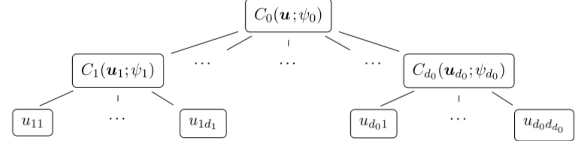
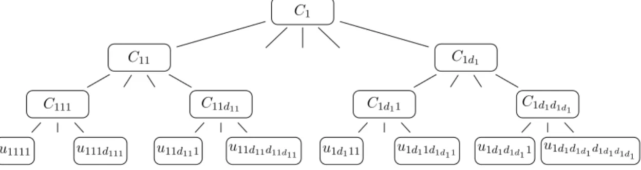
In the present work, we are mostly interested in a partially-nested Archimedean copula of the form
where, for all s1 œ {1,...,d0}, each Cs1 is a ds1-dimensional copula generated by Âs1, qd0
s1=1ds1 = d and us1 = (us11, . . . , us1ds1)T. Its structure can be depicted in the form a tree as in Figure 2.1. C0(u;Â0) C1(u1;Â1) u11 . . . u1d1 . . . . . . . . . Cd0(ud0;Âd0) ud01 . . . ud0dd0
Figure 2.1: Tree structure of a d-dimensional partially nested Archimedean copula with
qd0
s1=1ds1 = d.
Observe that the copula (2.5) has the following alternative representations. If one denotes
˚
Â0s1 = Â0≠1¶ Âs1
then Equation (2.5) can be developed into
C(u) = Â0 3ÿd0 s1=1 Â0≠1 5 Âs1 ;ds1 ÿ s2=1 Âs≠11 (us1s2) <64 = Â0 5ÿd0 s1=1 ˚ Â0s1{ts1(us1)} 6 =⁄ Œ 0 exp 3 ≠v0 5ÿd0 s1=1 ˚ Â0s1{ts1(us1)} 64 dF0(v0) =⁄ Œ 0 d0 Ÿ s1=1 Â0s1{ts1(us1);v0}dF0(v0),
where, for all s1œ {1,...,d0}
Â0s1(t;v0) = exp[≠v0Â0{Âs1(t)}] = exp{≠v0Â˚0s1(t)} and ts1(us1) = ds1 ÿ s2=1 Âs≠11 (us1s2).
We refer to Â0s1 as inner generator. It is a proper generator in t for each v > 0 as a
composition of the completely monotone function f(t) = exp(≠vt) with ˚Â0s1 which has
a completely monotone derivative, since ◊0Æ ◊s1.
The copula C0 is referred to as root (or outer) copula and each Cs, s œ {1,...,d0}, as
U1 0.6 0.8 1.0 0.6 0.8 1.0 0.0 0.2 0.4 0.0 0.2 0.4 U2 0.6 0.8 1.0 0.6 0.8 1.0 0.0 0.2 0.4 0.0 0.2 0.4 U3 0.6 0.8 1.0 0.6 0.8 1.0 0.0 0.2 0.4 0.0 0.2 0.4 U4 0.6 0.8 1.0 0.6 0.8 1.0 0.0 0.2 0.4 0.0 0.2 0.4
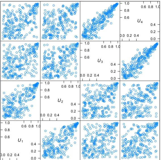
Figure 2.2: Pairwise scatterplots of 250 simulated points from a four-dimensional hier-archical nested Archimedean copula C0{C1(u1, u2),C2(u3, u4)} with Gumbel generators.
if U ≥ C the pair (Usj, Usk)T(j ”= k) has joint copula Cs whereas the pair (Urj, Usk)T (r ”= s) follows the root copula C0. Thanks to the R package nacopula, a scatterplot of
250 realization of a random variable U ≥ C0{C1(u1, u2),C2(u3, u4)} is provided in Figure
??.
More complicated nesting structures can be constructed. For example, one can ob-viously expand copula (2.5), by replacing each (Archimedean) copula Cs1 by a nested
Archimedean copula of the form (2.5). Hofert and Scherer (2011) used (2.5) to price Credit Default Swaps (CDOs), complex financial derivatives, which take effect when entities default on their loans.
The class of nested Archimedean copulas was first considered in (Joe, 1997, pp. 87) in the three- and four-dimensional case and later by McNeil (2008) in the general d-dimensional cases. McNeil (2008) and Hofert (2011a) derive an explicit stochastic rep-resentation for nested Archimedean copulas which allows for fast sampling similar to the Marshall-Olkin algorithm for Archimedean copulas. Hofert (2011b) provides efficient sampling strategies for the most important ingredients to this algorithm, the random variables responsible for introducing hierarchical dependencies. An implementation for several well-known Archimedean families (and transformations of such) is provided by the R package nacopula; see Hofert and Mächler (2011).
A sufficient condition under which (2.5) is indeed a proper copula is that the node ˚
Â0s= Â0≠1¶ Âs
has a completely monotone derivative; see McNeil (2008). Note that this sufficient nesting
condition is indeed only sufficient but not necessary. For example, if Â0(t) = ≠log(1 ≠ (1 ≠ e≠◊0)exp(≠t))/◊0 denotes the generator of a Frank copula and Â1(t) = (1 + t)≠1/◊1
the generator of a Clayton copula, then C(u) = C0(u1, C1(u2, u3)) is a valid (nested
Archimedean) copula for all ◊0, ◊1 such that ◊0/(1 ≠ e≠◊0) ≠ 1 Æ ◊1 although ˚Â01 is not
completely monotone for all parameters ◊0, ◊1. Following this example, one could ask
the following question: If one sets the outer generator Â0, what is the set of possible
compatible generators Âs so that ˚Â0s has completely monotone derivative? Hering et al. (2010) gives the answer and the set is given by
MÂ0= ; Âs|Âs(x) = Â0)µx+ ⁄ Œ 0 (1 ≠e xt)‹(dt)*,
where µ Ø 0 and ‹ is a measure on (0,Œ) satysfing⁄ Œ
0 min{1,t}‹(dt) < 0,
and either µ > 0 or ‹{(0,1)} = Œ, or both<.
As mentioned before, although nesting is possible in more complicated ways, we will mainly focus on nested Archimedean copulas of Type (2.5) (with some sectors possibly shrunk to single arguments of C0) and assume that the Archimedean generators Âs,
sœ {0,...,d0}, belong to Œ, the set of all Archimedean generators which are completely
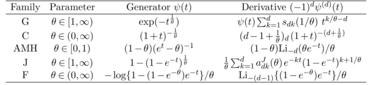
Table 2.I: Generator and its dth derivaties of the Gumbel, Clayton, Ali-Mikail-Haq , Frank and Joe copulas.
Family Parameter Generator Â(t) Derivative (≠1)dÂ(d)(t)
G ◊œ [1,Œ) exp(≠t1◊) Â(t)qd k=1sdk(1/◊) tk/◊≠d C ◊œ (0,Œ) (1 + t)≠1◊ (d ≠1+1 ◊)d(1 + t)≠(d+ 1 ◊)
AMH ◊œ [0,1) (1 ≠◊)(et≠ ◊)≠1 (1 ≠◊)Li
≠d(◊e≠t)/◊ J ◊œ [1,Œ) 1 ≠(1≠e≠t)1◊ 1 ◊ qd k=1aJdk(◊)e≠kt(1 ≠e≠t)k+1/◊ F ◊œ (0,Œ) ≠log{1 ≠ (1 ≠ e≠◊)e≠t}/◊ Li≠(d≠1){(1 ≠ e≠◊)e≠t}/◊
2.3 Parametric Archimedean Families
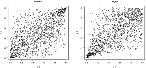
Among the most widely used parametric Archimedean families are those of Ali-Mikhail-Haq, Clayton, Frank, Gumbel, and Joe. These five families already provide a great flexibility in statistical modeling. A sample of one thousand points are provided in Figure 2.3, 2.4 and 2.5 in order to show on the one hand, how bivariate random vari-ables can differ even with the same measure of association and on the other hand to show the differences of these families. Ali-Mikhail-Haq copula is provided but the range of its Kendall’s tau is restricted to [0,1/3).
These one-parameter families can easily be extended to allow for more parameters. A great amount of work and effort have been done to construct new copulas, by creating generators with more parameters. Hofert (2010) provided a transformation called the
tilted outer power transformation which consists of using the generator ˜Âdefined as
˜
Â(t) = Â{(c–+ t)–≠ c},
where  œ Œ, – Ø 1 and c Ø 0. This yields a proper generator because the function (c–+ t)–≠c is nonnegative and has a completely monotone derivative. Since the composition of two completely monotone functions is still completely monotone, ˜Â is indeed completely
monotone. If c = 0, then it yields the commonly called outer power transformations. This paradoxical nomenclature comes from the fact that this transformation was first applied to Ï.
Using a slightly different version of (2.4), Hofert (2010) derived a semi-closed formula for the Kendall’s tau of the copula generated by ˜Â and showed that with the Clayton
copula, one could set parameters such that the theoretical values of both tails coefficients match their respective estimators. Alternatively, one could also fit a parameter in order to reproduce the value of one of the tails coefficients and then fit the second in order to match the theoretical value of the Kendall’s tau to the observations.
It is interesting to observe that the densities of the Frank, Gumbel, Joe and Ali-Mikhail-Haq copulas have only been discovered recently in Hofert et al. (2011b). Numer-ical implementation of these also requires a lot of attention, since in high dimensions, the density function numerically explodes for a large range of inputs.
Table 2.II: Inverse of the generator and its first derivative of the Gumbel, Clayton, Ali-Mikail-Haq , Frank and Joe copula.
Family Inverse Â≠1(t) Derivative of the Inverse (Â≠1)Õ(t)
G (≠logt)◊ ◊(≠logt)◊≠1/t
C t≠◊≠ 1 ◊t≠(1+◊)
AMH log{1≠◊(1≠t)}≠log(t) (1 ≠◊)/[t{1≠◊(1≠t)}]
J ≠log{1 ≠ (1 ≠ t)◊} ◊(1 ≠t)◊≠1/{1 ≠ (1 ≠ t)◊} F ≠log{1 ≠ exp(≠◊t)} + log{1 ≠ exp(≠◊)} ◊exp(≠◊t)/{1≠exp(≠◊t)}
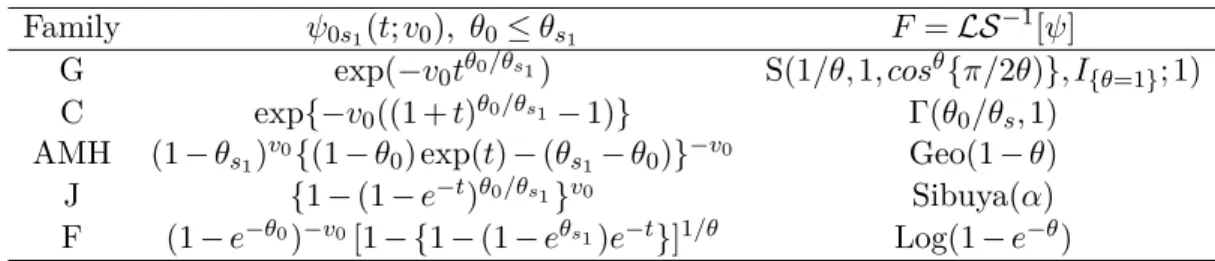
Table 2.III: Inner generator and the distribution F = LS≠1[Â] of the Gumbel, Clayton,
Ali-Mikail-Haq , Frank and Joe copula.
Family Â0s1(t;v0), ◊0Æ ◊s1 F= LS≠1[Â]
G exp(≠v0t◊0/◊s1) S(1/◊,1,cos◊{fi/2◊)},I
{◊=1};1)
C exp{≠v0((1 + t)◊0/◊s1≠ 1)} (◊0/◊
s,1) AMH (1 ≠◊s1)v0{(1 ≠ ◊0)exp(t) ≠(◊s1≠ ◊0)}≠v0 Geo(1 ≠◊)
J {1 ≠ (1 ≠ e≠t)◊0/◊s1}v0 Sibuya(–)
F (1 ≠e≠◊0)≠v0[1 ≠{1≠(1≠e◊s1)e≠t}]1/◊ Log(1 ≠e≠◊)
Tables 2.I and 2.III present known one-parameter Archimedean families with gener-ators  œ Œ. In these tables, one can find:
– an abbreviation of the name of the family of copula, that is ”G” (Gumbel), ”C” (Clay-ton), ”AMH” (Ali-Mikhail-Haq), ”J” (Joe), ”F” (Frank);
– the parameter space of the family;
– the families’ generator, their inverse and their derivatives;
– the explicit form of Â0s1(t; v0) = exp[≠v0Â0≠1{Âs1(t)}] where Â0 and Âs1 are from the
same family and the parameter respect ◊0Æ ◊s1;
– the distribution F = LS≠1[Â] whose Laplace-Stieltjes transform yields the generator Â.
Observe that the function Â0s(t; v0) will play a central role when the density of the
nested Archimedean copula (2.5) will be computed. The condition ◊0Æ ◊sis a compulsory restriction if one desires ˚Â0s= Â≠10 ¶ Âs to be completely monotone.
as sdk(x) = (≠1)d≠k d ÿ j=k xjs(d,j)S(j,k)
where s and S are the Stirling numbers of the first and second kind, respectively, given by the recurrence relations
s(n + 1,k) = s(n,k ≠1)≠ns(n,k), S(n + 1,k) = S(n,k ≠1)+kS(n,k),
for all k œ N, n œ N0, with s(0,0) = S(0,0) = 1 and s(n,0) = s(0,n) = S(n,0) = S(0,n) = 0
for all n œ N. Observe that the function snk(◊) is numerically challenging to evaluate, however this issue is resolved in the R package nacopula. The distribution F = LS≠1[Â]
of the Gumbel family is the stable distribution S(–,—,“,”,;1). An heuristic definition of a stable distribution is that if X and Y are of the same type, that is, one is a location scale transformation of the other, then their sum X + Y is still of the same type; see (Nolan, 2011, p. 4) for more details. It is also usual to define the stable distribution S(–,—,“,”,;1) by its characteristic function
„(t) = exp[i”t ≠“–|t|–{1 ≠ i— sign(t)w(t,–)}]
where w(t,–) = 1(– ”= 1)tan(–fi/2) ≠ 1(– = 1)2log(|t|)/fi. Stable laws have been exten-sively used to model financial (log-)returns thanks to their flexibility. Note that the Gumbel family is the only Archimedean extreme-value copulas that is Ct(u1/t) = C(u) for all positive t, see (Nelsen, 2007, p. 143). Interestingly, , the independence copula, can be considered as member of the Gumbel family. Indeed, the Gumbel copula with parameter ◊ = 1 has as generator Â(t) = exp(≠t), which is the generator of .
Concerning the Clayton copula, (d)k denotes the so-called falling factorial which is given by d(d ≠1)·(d≠k +1) = d! (d ≠k)! = k! A d k B = (d + 1) (d ≠k +1), where (–) =⁄ Œ 0 x –≠1e≠xdx
is the celebrated Euler’s gamma function. (–,—) denotes the gamma distribution with shape parameter – Ø 0 and scale — > 0. This law is often represented with its density function given by
f(x) = x
–≠1
(–)—–e≠—x.
The Clayton copula appeared in Clayton (1978), however bears the name of Cook and
Johnson copula in Genest and MacKay (1986).
0.0 0.2 0.4 0.6 0.8 1.0 0.0 0.2 0.4 0.6 0.8 1.0 Gumbel U_1 U_2 0.0 0.2 0.4 0.6 0.8 1.0 0.0 0.2 0.4 0.6 0.8 1.0 Clayton U_1 U_2
Figure 2.3: One thousand simulated points from the Gumbel and Clayton copula with parameter ◊ corresponding to a Kendall’s tau of 0.5.
0.0 0.2 0.4 0.6 0.8 1.0 0.0 0.2 0.4 0.6 0.8 1.0 Joe U_1 U_2 0.0 0.2 0.4 0.6 0.8 1.0 0.0 0.2 0.4 0.6 0.8 1.0 Frank U_1 U_2
Figure 2.4: One thousand simulated points from the Joe and Frank copula with parameter
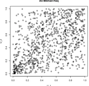
0.0 0.2 0.4 0.6 0.8 1.0 0.0 0.2 0.4 0.6 0.8 1.0 Ali-Mikhail-Haq U_1 U_2
Figure 2.5: One thousand simulated points from the Ali-Mikhail-Haq Copula with pa-rameter ◊ corresponding to a Kendall’s tau of 0.3
analysis. The function Li≠(d≠1)(x) denotes the Polylogarithm function, also known as
Jonquière’s function, and is defined for – œ Z as
Li–(x) =
Œ
ÿ
k=1
xk/k–.
For d œ N, Wood (1992) derived the alternative expression
Li≠d(x) = (≠1)d+1
dÿ+1 k=1
(k ≠1)!S(d+1,k)31 ≠x≠1 4k.
The inverse Laplace-transform of  is given by the geometric distribution Geo(p) with probability of success p œ (0,1]. This discrete law is usually given by its probability mass function pk= (1 ≠p)k≠1p for k œ N.
Concerning the Joe copula, it appeared in Joe (1993). The function aJ
dk(◊) appearing in the generator’s derivative is defined by
aJdk(◊) = S(d,k)(k ≠1≠1/◊)k≠1= S(d,k) (k ≠1/◊)(1 ≠1/◊), kœ {1,...,d}.
The distributional law originating Joe copula’s generator is the discrete Sibuya
distribu-tion Sibuya(p) with probability mass funcdistribu-tion pk=!pk"(≠1)k≠1 for k œ N.
Finally, Frank’s family was studied in Frank (1979) where the author also shows that this family is the only radially symmetric family among the Archimedean copulas. The distribution F = LS≠1[Â] is the logarithmic law Log(p), with parameter p œ (0,1] and
probability mass function pk= pk/{≠k log(1 ≠ p)}, for k œ N.
The interested reader can consult Hofert et al. (2011b), Hofert (2010) and the ref-erences therein for explicit or semi-explicit forms for Kendall’s tau or tail-dependence coefficients, as well as for more details about the content of this section.
DENSITIES OF NESTED ARCHIMEDEAN COPULAS
In this chapter, we first recall the notation and restate some useful results. We then tackle the problem by first deriving a convenient form for nested Archimedean copulas of Type (3.1) described below. This will allow us to compute their densities. The general strategy is presented in Section 3.2 and all necessary details for several well-known Archimedean families are provided. Section 3.4 addresses numerical evaluation of the log-density. Section 3.5 studies the behavior of the density when we set a third level of nesting.
3.1 Introduction
There has recently been interest in multivariate hierarchical models, that is, models that are able to capture different dependencies between and within different groups of random variables. One such class of models is based on nested Archimedean copulas. A
partially nested Archimedean copula C with two nesting levels and d0 groups, is given by C(u) = C0{C1(u1),...,Cd0(ud0)}, u = (u1, . . . , ud0)T, (3.1)
where d0denotes the dimension of C0and each copula Cs, s œ {0,...,d0}, is Archimedean with some generator Âs, that is,
Cs(us) = Âs{Â≠1s (us1) + ···+Âs≠1(usds)} = Âs{ts(us)}, s œ {0,...,d0}; (3.2)
here and in the following we denote
ts(us) = ds ÿ
j=1
Âs≠1(usj).
The copula C0 is referred to as root (or outer) copula and each Cs, s œ {1,...,d0}, as
sector copula. For Archimedean copulas, the density (if it exists) is theoretically trivial
to write down; for (3.2), one obtains
cs(us) = Âs(d){ts(us)} ds Ÿ j=1 (Â≠1 s )Õ(usj), usœ (0,1)d.
However, as already stressed, the appearing generator derivatives Â(d)s are non-trivial to access theoretically and, even more, computationally. This issue has recently been solved for several well-known Archimedean copulas and transformations of such; see Hofert et al. (2011b). Our goal is to extend these results to corresponding nested Archimedean copu-las. Note that this is more challenging because differentiating (3.1) is more complicated due to the inner derivatives that appear when applying the Chain Rule; in contrast to
Archimedean copulas, these inner derivatives depend on variables with respect to which one has to differentiate again. Already in low dimensions the corresponding formulas for the density c become challenging to write down and, even more, to evaluate in a numerically stable way.
3.2 Inner generator derivatives and densities for two-level nested Archime-dean copulas
3.2.1 The basic idea
Let C be a d-dimensional nested Archimedean copula of Type (3.1) (with some child copulas possibly shrunk to single arguments of C0) and assume the sufficient nesting
condition to hold; for the families Ali–Mikhail–Haq, Clayton, Frank, Gumbel, and Joe, this is fulfilled as long as all generators belong to the same family and ◊0 Æ ◊s, s œ {1,...,d0}. This condition implies that each copula Cs, s œ {1,...,d0}, is more concordant than C0.
One of the main ingredients we need in the following is the function
Â0s(t;v) = exp{≠v˚Â0s(t)} (3.3)
which we refer to as inner generator. It is a proper generator in t for each v > 0 as a com-position of the completely monotone function f(t) = exp(≠vt) with ˚Â0s which has a
com-pletely monotone derivative. The corresponding inverse is Â≠1
0s (u;v) = ˚Â≠10s{(≠log u)/v} = Â≠1s #Â0{(≠log u)/v}$, so that
Â≠1s (u) = Â0s≠1{G0(u;v);v},
where G0(u;v) = exp{≠vÂ0≠1(u)}. Note that G0 is a distribution function in u œ [0,1] for
any v > 0. With F0= LS≠1[Â0], we thus obtain
C(u) = C0{C1(u1),...,Cd0(ud0)} = ⁄ Œ 0 exp 5 ≠v0 d0 ÿ s=1 ˚ Â0s{ts(us)} 6 dF0(v0) =⁄ Œ 0 d0 Ÿ s=1 Â0s{ts(us);v0}dF0(v0) (3.4) =⁄ Œ 0 d0 Ÿ s=1 Â0s 5ÿds j=1 Â≠10s{G0(usj;v0);v0};v0 6 dF0(v0). (3.5)
Representation (3.5) provides a simple F0-mixture representation of C of the form
C(u) = ⁄ Œ 0 d0 Ÿ s=1 C0s{G0(us1;v0),...,G0(usds;v0);v0}dF0(v0) (3.6) = E5Ÿd0 s=1 C0s{G0(us1;V0),...,G0(usds;V0);V0} 6 , (3.7)