HAL Id: hal-01480980
https://hal.archives-ouvertes.fr/hal-01480980
Submitted on 2 Mar 2017
HAL is a multi-disciplinary open access
archive for the deposit and dissemination of
sci-entific research documents, whether they are
pub-lished or not. The documents may come from
teaching and research institutions in France or
abroad, or from public or private research centers.
L’archive ouverte pluridisciplinaire HAL, est
destinée au dépôt et à la diffusion de documents
scientifiques de niveau recherche, publiés ou non,
émanant des établissements d’enseignement et de
recherche français ou étrangers, des laboratoires
publics ou privés.
Numerical validation framework for micromechanical
simulations based on synchrotron 3D imaging
Ante Buljac, Modesar Shakoor, Jan Neggers, Marc Bernacki, Pierre-Olivier
Bouchard, Lukas Helfen, Thilo F. Morgeneyer, François Hild
To cite this version:
Ante Buljac, Modesar Shakoor, Jan Neggers, Marc Bernacki, Pierre-Olivier Bouchard, et al..
Nu-merical validation framework for micromechanical simulations based on synchrotron 3D imaging.
Computational Mechanics, Springer Verlag, 2017, 59 (3), pp.419-441. �10.1007/s00466-016-1357-0�.
�hal-01480980�
(will be inserted by the editor)
Numerical Validation Framework for Micromechanical
Simulations based on Synchrotron 3D Imaging
Ante Buljac · Modesar Shakoor · Jan Neggers · Marc Bernacki · Pierre-Olivier Bouchard · Lukas Helfen · Thilo F. Morgeneyer · Fran¸cois Hild
Received: date / Accepted: date
A. Buljac, Y. Neggers, F. Hild∗
Laboratoire de M´ecanique et Technologie (LMT), ENS Saclay / CNRS / Univ.
Paris-Saclay
61 avenue du Pr´esident Wilson F-94235 Cachan Cedex, France
∗Corresponding author. Email: [email protected]
A. Buljac, T. Morgeneyer
MINES ParisTech, PSL Research University, Centre des Mat´eriaux, CNRS UMR 7633, BP 87,
91003 Evry, France
M. Shakoor, M. Bernacki, P.-O. Bouchard
MINES ParisTech, PSL - Research University, CEMEF - Centre de mise en forme des
mat´eriaux, CNRS UMR 7635, CS 10207 rue Claude Daunesse 06904 Sophia Antipolis Cedex,
France L. Helfen
ANKA/Institute for Photon Science and Synchrotron Radiation Karlsruhe Institute of Tech-nology (KIT), D-76131 Karlsruhe, Germany
L. Helfen
Abstract A combined computational - experimental framework is introduced herein to validate numerical simulations at the microscopic scale. It is exemplified for a flat specimen with central hole made of cast iron and imaged viain situ syn-chrotron laminography at micrometer resolution during a tensile test. The region of interest in the reconstructed volume, which is close to the central hole, is an-alyzed by Digital Volume Correlation (DVC) to measure kinematic fields. Finite Element (FE) simulations, which account for the studied material microstructure, are driven by Dirichlet boundary conditions extracted from DVC measurements. Gray level residuals for DVC measurements andFE simulations are assessed for validation purposes.
Keywords Level set · Microstructure meshing · Multiscale analysis · Volume correlation·X-ray laminography
1 Introduction
In many applications, metals and alloys for in-use analyses and metal forming raise important issues for ductile fracture, which have led researchers to investigate more and more advanced damage models. A first category of damage models, known as macroscopic models [31, 52, 38], is used to predict not only damage occurrence but also the softening and transition to fracture. Due to their macroscopic nature, these models are known to have limited predictive capabilities and are usually calibrated and applied for specific loading conditions. For applications such as material forming, where loading may be complex and non proportional, these limitations are problematic [14, 13].
A promising alternative is provided by microscopic models [20, 47], where the macroscopic constitutive behavior is derived thanks to the homogenization of mi-croscopic calculations. This derivation may be purely analytical [20] or aided by numerical calculations on ideal microstructures [47]. However, the predictive ca-pabilities of these microscopic models are also known to be limited for arbitrary loading conditions [14, 13], due to quite restrictive assumptions that are used for their derivation [20, 47]. The calibration of these models is a challenging task that is being addressed in the literature using more advanced experimental and numerical procedures. Some variables such as porosity can now be observed experimentally thanks to X-ray imaging techniques [1, 8, 69, 22] with the possibility of considering inclusions and voids individually based on manual [69] or automatic [22] proce-dures.
Further, simulations are necessary to experimentally relate observed quanti-ties such as porosity and number of fractured/debonded inclusions to mechanical variables such as plastic strain and stress-based criteria. These calculations at the microscale are usually conducted with idealistic microstructures and constitu-tive behavior, considering homogeneous kinematic or static boundary conditions, which cannot capture the local strain and stress states that inclusions and voids are subjected to, due to their random shapes and distribution [1, 44, 66, 22]. The effect of the three-dimensional random distribution of voids on softening has been studied [18] using different void volume fractions.
The main objective of the current work is to enable for more realistic micro-scopic calculations thanks to physical models calibrated directly at the microscale to analyze the three steps of ductile damage, namely, void nucleation, growth and coalescence. To achieve such goal, a first step consists of developing a numerical
framework allowing for such validation and identification. The proof of concept of such validation framework is the topic of the present paper. The studied material is nodular cast iron, which at the microscale features a ferritic matrix and graphite nodules, with no significant porosity in the initial state. Then, under tensile load-ing, ductile fracture is mainly driven by a very early debonding of the nodules from the matrix, and coalescence of the subsequent nucleated voids [17, 29, 68]. Evidence in the literature [17, 74, 6, 29] suggests to model the nodules as voids, as their load carrying capacity is very low under tensile loading. This assumption is made herein and at the microscale the material is considered as a two-phase microstructure with a ferritic matrix and voids.
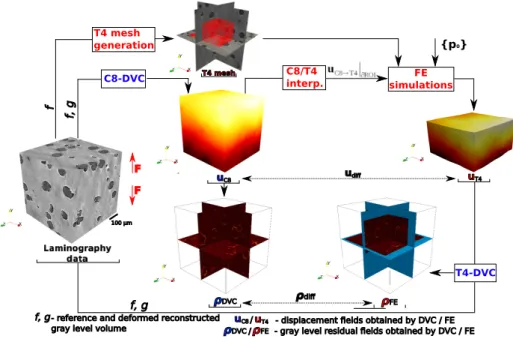
The final objective of the present work includes enabling for discussions regard-ing such assumptions, thanks to accurate and local error measurements directly at the microscale. This would help the development of experimentally probed microscopic models that could then be used to improve the common knowledge and understanding of ductile fracture, and deduce more accurate macroscopic re-sponses. In particular, the ultimate aim is to set up a framework that allows failure and coalescence mechanisms and criteria such as internal necking or coalescence via nucleation of voids on a second population of particles [30, 28] to be assessed numerically. The methodology proposed to obtain these local comparisons between experimental analyses and numerical simulations is based on the following steps (Figure 1):
– X-ray laminography to get 3D pictures of an in-situ test in a synchrotron facility. By post-processing them, one may get, for instance, a first estimate of the morphology of the two-phase microstructure.
– Global digital volume correlation (DVC) to measure displacement fields whose kinematic basis is made of the shape functions of 8-noded elements. These displacement fields serve two purposes. First, they correspond to the kinematic data of the test. Second and more importantly, they will be used as Dirichlet boundary conditions of Finite Element (FE) simulations at the microscale. – The FE simulations at the microscale explicitly account for the morphology of
the studied two-phase material. Therefore the mesh made of 4-noded tetrahe-dra is adapted to the microstructure with a Level-Set (LS) procedure. – FE simulations are run with an elastoplastic constitutive equation to model
the nonlinear behavior of the matrix.
– Comparisons between experimental measurements and numerical simulations are carried out for the displacement fields and correlation residuals.
C8-DVC ρDVC C8/T4 interp. FE simulations {p0} uC8 T4-DVC ρdi Laminography data ρFE f, g f, g f T4 mesh generation T4 mesh uT4 udi F F uC8 uT4 ρDVC ρFE
- displacement elds obtained by DVC / FE - gray level residual elds obtained by DVC / FE
f, g- reference and deformed reconstructed gray level volume //
100 µm
Fig. 1 Schematic representation of the methods used in the present paper for validating
Synchrotron radiation computed laminography is a non-destructive 3D imag-ing technique for scannimag-ing regions in laterally extended 3D objects [25, 24, 43, 12, 54]. This geometry is of particular interest in the field of mechanics of materials since sheet-like samples allow for a wide range of engineering-relevant boundary conditions. Laminography is related to the inclination of the specimen rotation axis with respect to the beam direction with an angle θ < 90◦; while tomogra-phy, as a special case of laminogratomogra-phy, is performed at the 90◦ angle during the scanning procedure and requires stick-like samples. However, due to the rotation axis inclination angle, incomplete sampling of the 3D Fourier domain of the spec-imen is performed and additional artifacts are present [23] but often they are less disturbing than the ones of tomography [72].
Laminography and tomography are nondestructive imaging techniques that are used in material sciences. They enable the material microstructures and their degradation mechanisms to be assessed qualitatively and quantitatively [41].In-situ experiments can also be performed to analyze the mechanical behavior of different materials [21, 11, 32, 15]. Initially developed at synchrotron facilities [3], these tests are also performed at lab tomography set-ups [10]. The 3D images are acquired at different steps of the loading history while the tested material is still under load for visualization and measurement purposes. For instance, 3D displacement fields can be measured via DVC.
DVC is a registration technique to measure 3D displacement fields in the bulk of samples. In its early developments [2, 62, 7, 70], DVC consisted ofindependently registering small interrogation volumes in the considered Region of Interest (ROI). This type of approach is nowadays referred to aslocal,i.e., the only information that is kept is the mean displacement assigned to each analyzed Zone of Interest
(ZOI) center. Various kinematic hypotheses, possibly accounting for ZOI warping, have been implemented. However, they are different from those made in FE sim-ulations in which the field is continuous and dense over the whole ROI. Global approaches, which appeared more recently [58], consist of performing registrations over the whole ROI by using kinematic fields based on finite element discretiza-tions. Such DVC approaches can be directly linked with numerical simulations of mechanical problems [53, 9].
Examples of techniques enabling real microstructures to be meshed can be found in the literature [75, 73]. Solutions are yet to be formulated to reduce the cost of these procedures both in terms of memory requirements and computation time. The LS method [49] is a useful tool to represent interfaces in an FE simulation when large deformations and complex topological events occur [63, 57, 51], though some regularity [61] and conservation [60] issues have to be handled. Distance maps and LS functions have also been used in the field of image processing to extract interfaces and topological data [34]. If FE simulations are to be performed with these interfaces, image processing can be performed directly on the FE mesh, thereby reducing memory requirements for high resolution images and enabling the parallel capabilities of standard FE codes to be used [61].
In the past, 3D meshes stemming from X-ray tomography data have been created for fatigue loading cases e.g. to assess the stress intensity factor ahead of a crack [53]. In Ref. [50] the 3D grain structure and orientation has been assessed via diffraction contrast tomography and subsequently been meshed in 3D to assess the effect of crystallographic orientation on fatigue crack propagation numerically and experimentally. To the best of our knowledge, there are no studies that explicitly mesh real microstructures for the case of ductile damage.
The paper is structured as follows. The experimental setup and the laminogra-phy imaging technique are first introduced. The basic principles of Digital Volume Correlation incorporating uncertainty quantification and DVC results are then presented. FE simulation tools including the microstructure meshing procedure and the strategy for applying DVC measured boundary conditions are described next. Last, the results from both methods are compared relatively via kinematic field subtractions and absolutely by computing gray level residuals.
2 Experimental analyses
2.1 In situ test
The material used in this study is a commercial nodular graphite cast iron (EN-GJS-400). The geometry of the flat specimen with a central hole is shown in Figure 2(a). The specimen geometry yields stress triaxialities within the range 0.4-0.5 in the vicinity of the central hole [56]. A stepwise loading procedure resulted in the force-displacement curve shown in Figure 2(b).
(a) 0 0.1 0.2 0.3 0.4 0.5 0.6 0.7 0.8 0.9 1 1.1 0 500 1000 1500 2000 2500 3000 F or ce [N] Screw displacement [mm] Load steps [-] 1 2 3 4 5 6 7 8 9 10 0 (b)
Fig. 2 (a) Schematic view of the sample with the scanned region close to the central hole. Section of the reconstructed volume with the position of the region of interest. (b) Macroscale force-displacement curve
The 3D images used herein were obtained at beamline ID15A [16] of the European Synchrotron Radiation Facility (Grenoble, France) with a filtered white beam (average energy around 60 keV), using 4,000 projections per scan. Due to the detector design and the angle between rotation axis and beam, the minimum specimen to detector distance is 70 mm. The resulting strongly contrasted edges are also expected to contribute to laminography artifacts typical for incomplete sampling. All these features induce increased DVC uncertainties compared with the measurement resolutions for tomography [45].
The testing device applies the load by controlling the displacement via manual screw rotation where grips incorporate a force measuring device. After apply-ing each loadapply-ing step, a scan is acquired while the sample is rotated about the laminographic axis (i.e.,parallel to the specimen thickness direction). This axis is inclined with respect to the X-ray beam direction by an angleθ ≈60◦. The series of radiographs acquired is then used to reconstruct 3D volumes via filtered-back projection [46]. The scanned region is positioned next to the central hole whose edge is used as orientation feature during the scanning procedure (Figure 2(a)). The reconstructed volume has a size of 1600×1600×1600 voxels. The physical size (length) of 1 cubic voxel is equal to 1.1µm.
2.2 Digital Volume Correlation
The correlation procedure using the whole volume size would be computationally too demanding. Therefore an extracted ROI of size 532×532×532 voxels is used for DVC analyses. The position of the ROI in the global coordinate system is
shown in Figure 2(a) while in thez direction the ROI and sample mid-thickness planes coincide.
2.2.1 Basic principles
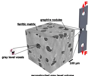
DVC used herein is an extension of 2D global Digital Image Correlation [4, 27]. The reconstructed volume is represented by a discrete scalar matrix of spatial coordinatexof (in this case 8-bit deep) gray levels determined by the microstruc-ture absorption of X-rays (Figure 3). The image contrast is mainly due to graphite nodules of micrometer size.
100 µm graphit nodules
ferritic matrix
F
F
gray level voxelsreconstructed gray level volume e
Fig. 3 Reconstructed volume as a spatial discrete matrix of gray level values
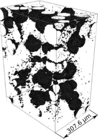
There are also smaller dark features in the ferritic matrix that can either be voids or graphite. To better appreciate their presence a typical 3D rendering of all dark features in nodular cast iron is shown in Figure 4. The image was obtained by using a Gaussian filter (radius = 1 voxel) and subsequent gray level thresholding. To quantify the presence of this second population of dark features an image analysis has been performed. The above presented thresholded volume serves as
input for an object counting procedure where all the large objects (i.e.,volumes >10×10×10 voxels, which is the minimum nodule size) are a priori discarded from the analysis. The objects in the remaining volume are counted and divided by the corresponding number of DVC elements (their volume being`3= 32×32× 32 voxels). If all segmented small particles are considered the average number of particles per element is 1.6. However, if particles smaller than 1 or 5 voxels are considered as noise, the values are 1.1 and 0.6 particle per element, respectively. Therefore there is contrast within the ferritic matrix that can be registered and allows displacement fields to be measured between nodules. Let us note that the filter has been applied to the 3D image, which has evened out voxel-scale contrast. Conversely, no filtering is performed for the correlation procedure and it may thus be expected that submicrometer contrast also contributes to the determination of the kinematic fields.
307.6 µm
The principle of DVC consists of registering the gray levelsf in the reference configurationx and those of the deformed configurationg, which satisfy
f(x) =g(x+u(x)) (1)
whereuis the displacement field. However, due to acquisition noise, reconstruction artifacts [72] and the correlation procedure itself [37], ideal match is not achieved in real examples. Consequently, the solution consists of minimizing the gray level residual
ρ(x) =f(x)− g[x+u(x)] (2)
by considering its L2-norm with respect to kinematic unknowns. Since a global approach is used herein [58],C0 continuity condition over the ROI is prescribed
to the solution and the global residual to be minimized reads
Φ2c= X
ROI
ρ2(x). (3)
The displacement field is parameterized by using a kinematic basis consisting of shape functionsΨp(x) and nodal displacementsup
u(x) =X p
upΨp(x). (4)
Among a whole range of available fields, finite element shape functions are partic-ularly attractive because of the link they provide between the measurement of the displacement field and numerical models [53]. Thus, a weak formulation based on C8 finite elements with trilinear shape functions is chosen [58]. After successive linearizations and corrections the current system to be solved reads
where
Mij = X
ROI
(∇f · Ψi)(x)(∇f · Ψj)(x) (6)
represents the DVC matrix, while vector{b}
bi= X
ROI
(f(x)−˜g(x))(∇f · Ψi)(x) (7)
contains the current difference between the reference volumef and the corrected deformed volume ˜g=g(x+ ˜u(x)), ˜ubeing the current estimate of the displacement field. The global residual needs to decrease so that convergence is achieved,i.e., the displacement corrections{δu}become vanishingly small.
In this form, the displacement field is regularized in the sense of a continuity requirement that is a priori assumed for the kinematic solution. Moreover, ad-ditional mechanical knowledge may be added to help convergence. This type of procedure is referred to as mechanical regularization [65]. In the present analyses, mechanical regularization based on the satisfaction of the elastic solution for the inner nodes in the calculated domain has been introduced. In the absence of body forces it implies
[K]{u}={0} (8)
where [K] is the rectangular stiffness matrix associated with the inner nodes. Displacement fields uthat do not satisfy the equilibrium will give rise to a gap that will be minimized in addition to the correlation residuals
Φ2m={u}t[K]t[K]{u}. (9)
Minimizing the equilibrium residuals incorporates the mechanical admissibility in the solution of the measured kinematic field. However, the previous strategy cannot be used as such for boundary nodes, except those that belong to a free edge. For
the other boundary nodes, an edge regularization is considered in the same way as what was recently proposed for 2D situations [67, 65]
Φ2b ={u}t[L]t[L]{u} (10)
where [L] behaves as a mathematical operator eliminating non-physical high fre-quency solutions. Since they do not have the same physical units these functionals cannot be added directly [36]. For this reason, a reference displacement field v is needed to normalize them. Additionally, weights wm and wb are given to the normalized functionals, thereby defining regularization lengths that act as cut-off wavelength of low pass mechanical filters [36]. The regularized correlation proce-dure consists of iteratively solving linear systems
([M] + [N]){δu}={b} −[N]{u} (11) where [N] =wm {v} t[M]{v} {v}t[K]t[K]{v}[K] t [K] +wb {v}t[M]{v} {v}t[L]t[L]{v}[L] t [L]. (12)
The normalization displacement fieldv is associated with a wave vectorkso that the two weights are defined as [65]
wm= (2πkkk`r)4, wb= (2πkkk`b)4 (13)
where `r and `b represent regularization lengths. By tuning the regularization length the influence of the mechanical regularization functional can be varied, resulting in more or less smooth fields. In strongly regularized solutions, high spatial frequencies are filtered out when not mechanically admissible as part of an elastic solution. Hence, the regularization procedure makes use of constitutive laws and helps correlation registration to converge even in the close to zero-gradient
gray level zones as found in the cast iron matrix. Finally, let us stress this does not imply that the final solution is elastic in nature, which will be observed in the case of cast iron. However, regularization can still be used as anad hoc solution to the problem, giving a rough, but fairly good estimate of the correct solution. This solution is then used as initial guess in the subsequent calculations with decreased regularization lengths. This so-called relaxation procedure [67] is followed herein until the overall weights put on Φm andΦb are equal to zero, i.e.,no additional requirements besides gray level conservation are assumed. During the relaxation procedure the`r/`b ratio was equal to one.
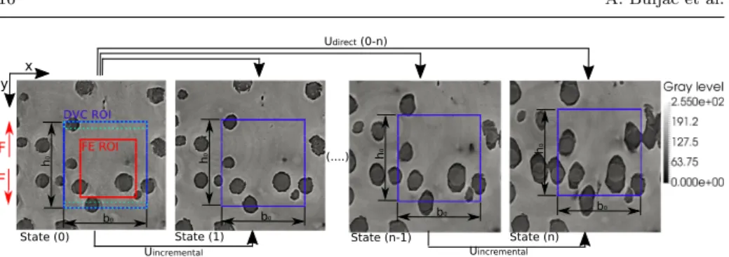
2.2.2 Direct vs. incremental DVC calculations
Since stepwise loading has been applied, direct DVC results refer to the solutions obtained by correlating the undeformed volume (state (0)) and the correspond-ing deformed configuration (state (n)), while incremental calculations stand for the correlation between any reference volume (state (n)) and subsequent (state (n+ 1)) configuration. Due to the small number of scans available for the experi-ment, high levels of displacements occur between two consecutive acquisitions. The convergence of direct DVC calculations is hardly achieved under such conditions, hence an incremental correlation procedure is followed (Figure 5).
State (0) State (1) State (n-1) State (n) (....) DVC ROI Udirect (0-n) Uincremental Uincremental h 0 b0 h 0 h0 h 0 b0 b0 b0 x y F F
Fig. 5 Difference between incremental and direct DVC procedures
Further, there are two different ways of displaying incremental calculation re-sults. First, the fields are shown in the reference configuration of each incremen-tal analysis. Second, all the results can be expressed in a Lagrangian way by re-projecting back all the measured incremental displacement fields on the unde-formed frame (by subtracting neighboring direct calculation results). In the sequel, the first approach will be used but special care has to be exercised to identify com-mon features to make the comparison objective.
All the results reported hereafter have required the DVC analyses to converge, namely, the root mean square (RMS) of the displacement increment between two iterations is less than 10−4 voxel. An additional check is related to the residualsρ that will be shown in the sequel.
2.2.3 Link between DVC and numerical simulations
The measured displacements are expressed on a regular undeformed mesh made of 8-noded cube elements. Full-field results written node-wise are provided as.txt output files of DVC and will be used as boundary conditions for the FE mechanical model. Hence, for the first incremental loading step (0)-(1) the results are written on the undeformed frame (0), for the second (1)-(2) on the mesh associated with
the microstructure at state (1), and so on. An example is shown in Figure 5. Since undeformed meshes (blue DVC ROI) with constant (initial) size are considered on the microstructure state (n −1) for loading step (n), with its positions defined relatively to the followed microstructure features, some of the material points present in the DVC ROI at the beginning are lost during the loading history. These regions are depicted with white dotted rectangles in the figure. Hence, if all the incremental displacement fields are cumulated to the initially defined nodes, it will end up with a partial solution. Since the material points used for FE computations need to possess a complete kinematic information through the loading history, just an inner part of the original ROI has been utilized for communication between DVC and FE simulations (red FE ROI), where the ROI size reduction especially refers to the loading direction (y) for which the displacements are the largest.
Once defined, boundaries of the domain are used to extract the corresponding part of the DVC displacement solutions. These displacements are interpolated on the unstructured tetrahedral mesh (T4 mesh) used in numerical simulations. They are used as Dirichlet boundary conditions in the FE simulations. Additionally, since the underlying experiment and consequently DVC calculations are obtained with a small number of loading steps, linear interpolation in time is necessary to properly prepare boundary conditions for FE computations.
2.3 Uncertainty quantification
Before presenting any result, an uncertainty assessment is performed. It consists in analyzing two consecutive scans of the unloaded and loaded sample without applying any additional load (i.e.,denoted “bis”) or prescribing rigid body motions
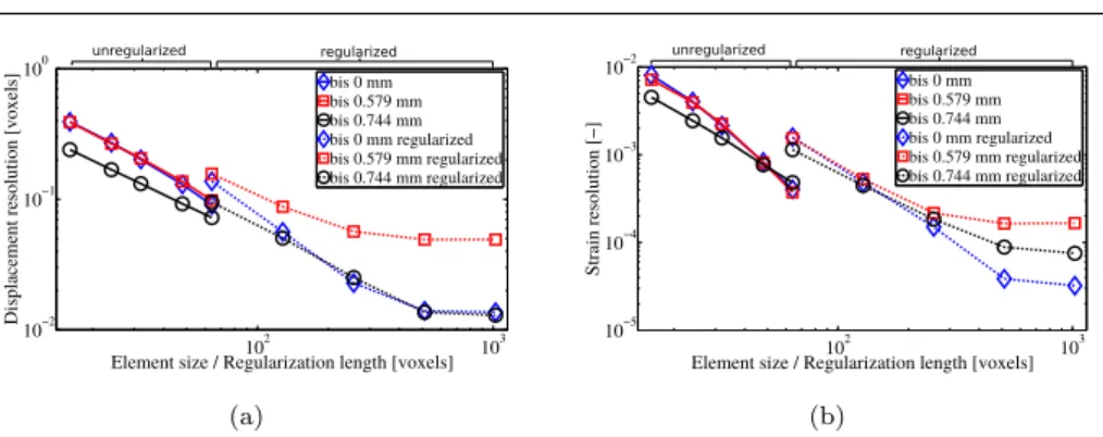
between the two acquisitions [45]. For the present experiment, three independent “bis” cases are available, namely, “0 mm” in the undeformed state and two more in deformed states: “0.579 mm” and “0.744 mm” of the screw displacement (see Figure 2(b)). Due to the noise contribution and reconstruction artifacts, these two volumes are not identical. Therefore, the measured displacement field accounts for the cumulated effects of laminography and DVC on the measurement uncertainty. From the mean gradient of the displacement field over each C8 element the Hencky strain tensor and its second invariant (i.e.,von Mises equivalent strain) will be used in the sequel.
The uncertainty values are evaluated by the standard deviation of the measured displacement and calculated strain fields. Figure 6 shows the standard displace-ment and strain uncertainty levels for the analyzed ROI. An increase of the spatial resolution (i.e., proportional to the element size or regularization length [36]) is followed by a decrease of the displacement/strain uncertainty since more voxels per nodal displacement are available. This first series of results shows that the convergence of unregularized DVC can be achieved with smaller elements than the 32-voxel limit discussed in Section 2.2.1 thanks to the fact that displacement fields are a prioriassumed to be continuous over the whole ROI. However to lower the measurement uncertainties, the element edge size was chosen equal to 32 voxels (or 35µm) in all three directions, which yields a standard displacement and equivalent strain resolution of 0.2 voxel and 0.2 %, respectively. These values represent the limit below which the measured levels are not trustworthy. As expected, these lev-els are greater than uncertainties reported in case of tomography obtained on cast iron scans [39] but lower than laminography results on less contrasted aluminium alloy microstructure [45].
102 103 10−2
10−1
100
Element size / Regularization length [voxels]
Displacement resolution [voxels]
bis 0 mm bis 0.579 mm bis 0.744 mm bis 0 mm regularized bis 0.579 mm regularized bis 0.744 mm regularized unregularized regularized (a) 102 103 10−5 10−4 10−3 10−2
Element size / Regularization length [voxels]
Strain resolution [ − ] bis 0 mm bis 0.579 mm bis 0.744 mm bis 0 mm regularized bis 0.579 mm regularized bis 0.744 mm regularized unregularized regularized (b)
Fig. 6 Standard displacement (a) and equivalent strain (b) resolutions as functions of the
element size or regularization length
It is worth noting that the chosen element size (i.e., `= 32 voxels) does not allow the kinematic details induced by the cast iron microstructure to be fully captured. However, the main purpose of the DVC calculations is to provide realistic boundary conditions to the FE simulations. It has been shown that such Dirichlet boundary conditions do not need to be measured at very fine spatial resolutions for identification and validation purposes. However, it is crucial that they capture the mesoscopic kinematics [26].
Keeping the element size identical (i.e., `= 24 voxels), the uncertainties can be further decreased (down to 0.05 voxel for displacements or 0.02 % for strains) by utilizing mechanical regularization [37, 65]. The results with mechanical regular-ization are shown with dashed lines in Figure 6. A significant gain in uncertainty is achieved since mechanical regularization successfully penalizes high-frequency noise features. A saturation is observed for regularization lengths greater than `r= 512 voxels. The observed differences are due to different initial quality of the underlying scans that originates from focal point shift that occurred during the experiment due to thermal drift (analyzing raw data reveals the best quality scans
are indeed in the “0.744 mm” case). Further, once damage sets in, higher gray level gradients are more favorable.
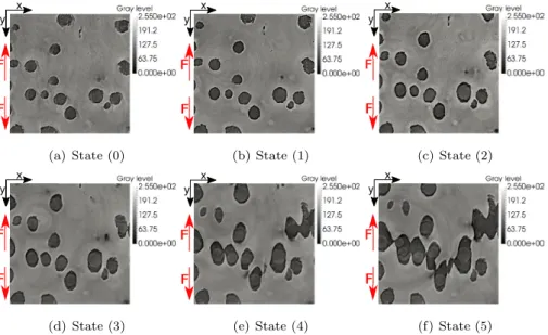
2.4 DVC results
Figure 7 shows microstructure sections for the unloaded state and after the first five loading steps. From the reconstructed raw images early nodule debonding from the matrix is noted. This phenomenon was also observed in the residual maps of DVC analyses for another cast iron grade imaged via tomography [68]. From the macroscopic load-displacement curve it can be seen from the sixth loading step on that softening is followed by the final crack propagating through the scanned region and these results, although available, are of less interest for the present numerical modeling procedure. Conversely, the measured kinematic fields for the initial steps are of special interest.
F F x y (a) State (0) F F x y (b) State (1) F F x y (c) State (2) F F x y (d) State (3) F F x y (e) State (4) F F x y (f) State (5)
Fig. 7 Through thickness section showing nodules embedded in the matrix for the undeformed state (a) and after the first five loading steps (b)-(f)
2.4.1 Correlation residuals
While performing DVC calculations at each iteration the deformed volume g is being corrected by the current estimate of the displacement field. The final dif-ference between undeformed and corrected deformed volumes represents the gray level residual field ρ(x). It does not only serve as correlation quality inspector, but it also provides useful tools for sensitive (precise) detection of damage occur-rence [68]. In the present case it will also provide an objective way of comparing measured and simulated displacement fields, as will be shown hereafter.
The kinematic basis utilized herein prescribes C0 continuity to the
mea-sured displacement field. Any deviation from this requirement (e.g.,nodule/matrix debonding, void nucleation and growth) cannot be properly captured by the un-derlying kinematics and will be reflected in a local residual increase. Let us note that corrected volumes are updated at each iteration on a sub-voxel scale by using gray level interpolation (with a trilinear interpolation scheme). This means that by using residual fields one can benefit from sub-voxel resolution in the gray level registration procedure (Figure 6). However, a significant amount of damage growth deteriorates gray level conservation and possibly DVC convergence.
In Figure 8 the gray level residual fields for the first loading step are shown in isometric (a) and section (b) views as functions of different regularization lengths. It can be noted that areas of higher residuals correspond with the position of the debond zones. The relaxation procedure gives more freedom (since debonding and its consequences are far from the elastic assumptions and those of constant volume being made) in the correction of the deformed image as a part of the
DVC procedure that results in slightly lower residual levels for the non-regularized approach. F F x y z (a) `r= 512 voxels F F x y z (b) `r = 256 voxels F F x y z (c) `r= 0 voxel F F x y (d) `r= 512 voxels F F x y (e) `r = 256 voxels F F x y (f) `r = 0 voxel
Fig. 8 (a)-(c) Isometric view of the gray level residual field and (d)-(f) through thickness
section with the residual map for first loading step and three different regularization lengths
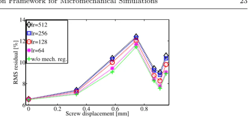
Beside debond zones with higher gray level residuals, the residual map in the rest of the ROI shows sufficiently low values indicating successfully converged DVC calculations. This is confirmed in Figure 9 where the root mean square (RMS) residual field is shown for all loading steps and various regularization lengths. Plotting the values for different regularization lengths shows the relaxation pro-cedure,i.e., decreasing elastic regularization, yields slightly better solutions since the elastic behavior requirements are relaxed. The fact that the residuals remain close to the levels observed in the uncertainty analysis is an additional proof of global convergence of DVC.
0 0.2 0.4 0.6 0.8 6 8 10 12 14 Screw displacement [mm] RMS residual [%] lr=512 lr=256 lr=128 lr=64 w/o mech. reg.
Fig. 9 Root mean square gray level residual (normalized by dynamic range of the volume
-256 gray levels) for various regularization lengths (expressed in voxels)
2.4.2 Displacement fields
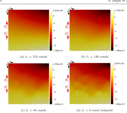
Displacement fields in the loading direction for the first loading step and four dif-ferent regularization lengths obtained through the relaxation procedure are shown in Figure 10. These fields correspond to the mid-thickness section of the sample. Only relaxed solutions allow the heterogeneities induced by the nodules to be captured. The mean values of the displacement fields do not differ much but the standard deviation is somewhat increased by decreasing the regularization lengths. This trend can be understood with the decrease of the registration residuals (see Figure 9). The relaxed solution (i.e., `r= 0) allows more kinematic heterogeneities that endow more precise corrections of the deformed images,i.e., lowers the dif-ference (especially in debond zones) with the undeformed image.
x y F F (a) `r= 512 voxels x y F F (b) `r = 128 voxels x y F F (c) `r= 64 voxels x y F F (d) `r= 0 voxel (relaxed)
Fig. 10 Displacement fields of mid-thickness section for the first loading step and four
dif-ferent regularization lengths
2.4.3 Equivalent strains
Equivalent strain maps are shown in Figure 11 for the first loading step during the relaxation procedure. Let us note the strain field heterogeneities can be seen starting from`r= 2`= 64 voxels.
x y F F (a) `r= 512 voxels x y F F (b) `r = 128 voxels x y F F (c) `r= 64 voxels x y F F (d) `r= 0 voxel (relaxed)
Fig. 11 Equivalent strain maps of mid-thickness section for the first loading step and four
different regularization lengths
The strain maps plotted over the corresponding microstructure details for first loading step for an unregularized solution are shown in Figure 12. It is interesting to note that even at this scale, from the first loading step on, higher strained areas are observed between some of the nodules. It is concluded that the presence of strained bands is always accompanied by nodules, while not all the nodules are affected by the localized strain pattern.
F F x y F F x y F F x y
Fig. 12 Equivalent strain maps plotted together with the corresponding microstructure
sec-tions for the first loading step (unregularized DVC) and different posisec-tions along the thickness direction
3 Mechanical simulations
Performing FE simulations with real microstructures and boundary conditions requires a robust and efficient numerical framework. Robustness is important be-cause a real microstructure includes complex features and interfaces. For example, a wide range of biomechanical problems typically requires meshes of human bones or tissues that are accurate enough to reproduce nature but with a mesh qual-ity that allows FE simulations at large strains [75, 73, 48]. Other materials such as foams and composites induce similar challenges as they feature complex and sometimes tortuous microstructures [33, 73]. In the present case, the microstruc-ture consists of voids (Figure 3) that are nearly spherical but of different sizes and with a random distribution where some voids may have initially coalesced. Additionally, realistic boundary conditions may induce a non proportional load-ing path and heterogeneous distortions of the FE domain. In the followload-ing, the whole numerical framework for performing the simulations is presented from the mesh generation to the application of boundary conditions and mechanical
mod-eling (Figure 1). Particular attention is paid to the computational cost of each operation as it will play a key role for computations on large ROIs.
3.1 Meshing X-ray images
Meshing real materials and structures from images is a challenging task for which multiple approaches have been proposed [75, 73]. A direct method would consist of first thresholding the image, then applying a contour detection algorithm to build a surface mesh of all interfaces and finally constructing a volume mesh around them [75]. The method used herein first builds a volume mesh, usually from a cube, which can be the image itself or, more likely, the ROI. Then, the image is imported into this mesh and surface meshes are built inside this volume mesh using mesh adaption techniques.
3.1.1 Image import
In general, the whole X-ray image is not considered because it is likely to contain some artifacts and/or noisy areas. A simple way to extract only the regions that are exploitable is to crop the image based on a 3D box. The first step of the meshing procedure is to generate a 3D mesh of this box. When no mesh refinement is used, the box can already be meshed with the chosen uniform isotropic size. When local mesh refinement is used, especially if it is based on geometric error estimators, it is assumed that the initial mesh of the 3D box is globally finer than the smallest size prescribed by this local mesh refinement. After import and meshing of the image, this mesh can be coarsened in areas where refinement is not necessary.
The next step is to have a description of the image in the mesh, for exam-ple through node-wise gray levels defined at mesh nodes. The image can also be
thresholded before import, in which case each gray level will represent not a color but a phase identifier. In order to transfer this information from the image to the mesh, FE interpolation is used. The image is considered as a hexahedral FE grid where voxels are nodes, and field transfer is operated from this grid to the nodes of the 3D box. For each node of the 3D box, finding the hexahedron of the image that contains it can be performed in constant time, since the image is a structured grid.
Once this gray level is obtained, LS reinitialization is performed. LS functions are a useful tool to localize evolving interfaces in multiphase simulations [49, 63, 51]. They play a key role in the numerical method that will be used to adapt the mesh throughout the simulations. The LS functionφi for phaseiis defined as
∀t, ∀x ∈ Ω(t), φi(x, t) = +d(x, ∂Ωi(t)), x ∈ Ωi(t), −d(x, ∂Ωi(t)), x /∈ Ωi(t), (14)
where Ω(t) is an evolving domain, Ωi(t) is the subset of Ω(t) occupied by phase i, and d(x, ∂Ωi(t)) is the Euclidean distance from point x to the boundary of Ωi(t). LS functions will also play a key role to compute the porosity and for error measurements as they carry all information regarding phase distributions. The difficulty is how to convert a node-wise gray level or phase identifier into a signed distance function. This problem is known as the LS reinitialization problem [64, 61]. It is solved herein using a direct brute-force algorithm enhanced with a parallel space partitioning technique [61]. Once LS functions are obtained for each phase of the domain, one may start a simulation using only this implicit representation of interfaces. The FE framework developed in Refs. [59, 60] aims at going a little farther and maintaining an explicit representation of interfaces throughout the simulation.
3.1.2 Mesh generation
Mesh generation is directly based on LS functions. Every edge where an LS func-tion φi has opposite signs on both ends is an edge crossed by an interface. In Ref. [59], an interface fitting procedure was proposed in order to introduce all these intersection points in the mesh of the domain. This procedure is likely to in-troduce very poor quality elements that will render any FE simulation on this mesh impossible. A mesh adaption step is therefore necessary to restore an appropri-ate mesh quality. In Ref. [60], the topological mesh adaption technique detailed in Ref. [19] was enhanced by taking into account volume conservation during remesh-ing in order to preserve (at best) the distribution of phases in the initial mesh. As presented in Section 3.5, it is also used during FE simulations, where large de-formations and topological events may induce large distortions of the Lagrangian mesh.
The whole image import and mesh generation procedure is summarized in Figure 13. A closer look at interfaces is presented on the right side of this figure. While interface fitting produces a smooth surface mesh of the interface, which is actually the zero-LS function, edge lengths are randomly distributed and element quality is deteriorated. This is corrected in the last mesh adaption step.
image interpolation level-set reinitialization fitting final adaptation
Fig. 13 Example of mesh generation from a 2D binary image
3.2 Definition of a computational domain
For each experiment, 3D X-ray images are reconstructed at various loading steps. For obvious reasons, it is impossible to systematically capture the same part of the specimen, and some features may go in and out of the images. Regarding DVC, this is dependent on whether computations are conducted with a direct or incremental scheme (see Figure 5). The ROI may be different depending on the used method as for example more material points of intermediary images are taken into account by the incremental method. However, this is not possible for
mechanical simulations, namely, the chosen initial FE domain has to remain inside all DVC ROIs throughout the simulation. This is independent of the DVC method (direct or incremental). In practice, the DVC ROI is chosen as large as possible (ideally, the full X-ray images minus the regions with missing information), and the FE domain for mechanical computations is manually chosen in order to be contained inside all DVC ROIs.
3.3 Application of boundary conditions
Once an appropriate domain has been chosen and meshed according to the ini-tial image, boundary conditions have to be applied to follow experimental images through each loading step. This problem is split into two operations that are time and spatial interpolations. Neither the time step nor the FE mesh used for me-chanical computations will generally match the loading steps used in experiments and the mesh used for DVC. In practice, a loading step will be split into several time steps, especially at crack initiation. Regarding the FE mesh, it will be fitted to the features of the microstructure as described in Section 3.1. It is worth noting that such fine meshes are not compatible with standard DVC approaches [36], the reason for that being the fact the number of voxels per nodal displacement cannot be arbitrarily reduced without additional regularization [37, 36] (see Figure 6). As discussed in Section 2.3, the very details of the displacement field are not needed for Dirichlet boundary conditions when used for validation purposes.
The application of boundary conditions is presented here for time t, which is not necessarily a time at which a scan was acquired, and for boundary nodes of the FE mesh, which are not necessarily nodes of the DVC mesh. Note that t is
an artificial and dimensionless time linked to the loading steps (i.e.,the material behavior is rate-independent). The automatic procedure implemented in the FE code reads:
1. find the two loading steps taken at instantsta and tb such thatta ≤ t < tb, with no loading step betweenta andtb,
2. read the undeformed DVC mesh and the DVC displacement field atta, 3. perform linear time-interpolation,
4. perform linear (resp. trilinear) space-interpolation by finding for each boundary node of the FE mesh the element of the DVC mesh containing it, and apply tetrahedral (resp. hexahedral) interpolation inside this element depending on its type.
Operation 1 has linear complexity and negligible cost as the number of loading steps is small. The same remark applies to operations 2 and 3 as the DVC mesh is at least one order of magnitude coarser than the FE mesh (in terms of number of elements). Operation 4, however, requires to localize each node of the FE mesh inside the DVC mesh. Optimized algorithms can be found in the literature to perform such operation in logarithmic time [61] but were not implemented here due to the small size of the DVC mesh compared to the FE mesh. Hence, this operation has a cost proportional to the number of elements in the DVC mesh, and quadratic cost considering it has to be run for all boundary nodes of the FE mesh. This cost would have to be optimized if finer DVC meshes were to be used, especially if those meshes were to have an order comparable to that of the FE mesh.
Last, the displacement field interpolated at the boundary nodes of the FE mesh is prescribed by means of Dirichlet boundary conditions on the whole boundary of the FE domain. Therefore, apart from small differences due to interpolation and remeshing, the boundary of the FE mesh is expected to follow exactly the measured displacement field at each loading steps. The errors that will be measured inside the domain are expected to be mainly due to the mechanical modeling.
3.4 Constitutive law
As stated in the introduction, graphite nodules are considered as voids in the present computations [17, 74, 6, 29]. These voids are modeled using an isotropic linear elasticity law with very low Young’s modulus. With a sufficiently low value, the behavior of a void is obtained. The influence of such penalization technique on void growth was investigated in Ref. [57]. This investigation is again carried out herein.
Regarding the ferritic matrix, von Mises plasticity with power law hardening is assumed [40]
σ0(ε) =σy+Kεn, (15)
where ε is the equivalent (von Mises) plastic strain, σy the yield stress, K the plastic consistency and n the hardening exponent. This law was fitted against a stress/strain curve for a pure ferritic matrix [74], which is assumed to be repre-sentative of thein-situbehavior of the ferritic matrix of the studied cast iron. The obtained values areσy= 290 MPa,K= 382 MPa,n= 0.35; the Young’s modulus E = 210 GPa, and Poisson’s ratio ν = 0.3. The chosen constitutive law may appear very simplistic. However, in virtually all unit cell calculations or
microme-chanical models accounting for ductile damage, such types of plasticity postulates are used. It is noteworthy that more complex models can be incorporated in the present framework (e.g., crystal plasticity).
To avoid numerical locking in the plastic regime, a mixed velocity-pressure formulation is used with a P1+/P1 element [5]. Additionally, a Newton-Raphson algorithm is implemented to account for the nonlinear behavior of the matrix [71]. This mechanical solution yields displacement fields at mesh nodes and stress / strain distribution at quadrature points, including the equivalent plastic strain. Large plastic strains are considered herein thanks to an updated Lagrangian for-mulation, which is commonly used in metal forming simulations [71]. This incre-mental formulation has proven to give accurate results for small time steps (time step convergence is usually carried out in such analyses as shown below).
3.5 Mesh motion / adaption
All FE computations are performed in a Lagrangian framework. Therefore, at each time step, the displacement field is applied to move the nodes of the mesh. A mesh adaption technique has already been introduced in order to restore mesh quality when generating body-fitted meshes from images. The same technique is applied during the FE simulation. Due to the presence of large void growth and coalescence events in the images, the boundary conditions may induce very large deformations, which can be local for specific voids, or global to the whole domain. Though no fracture or coalescence criteria such as those used in Ref. [59] are employed in the present simulations, these deformations may induce topological events such as coalescence of neighboring voids. The mesh motion and adaption
procedure described in Ref. [60] was designed to handle such issues. This procedure consists of detecting element flip during mesh motion, going back if it occurred, remeshing, and trying again. Doing so, small deformation steps are performed and the robustness of the Lagrangian framework is improved.
3.6 Simulation results
The DVC ROI for which boundary conditions are available is of dimensions up to 5323 voxels. Finding the largest 3D box included in this ROI and in all ROIs through each loading step was performed manually by launching simulations with-out meshing any microstructure. Box dimensions were reduced progressively until reaching the above condition. The chosen FE domain is of dimensions [−245,200]× [−17,200]×[−245,245] voxels, due to necking in thex-direction and crack opening in they-direction.
In the following, FE simulation results are presented using this initial domain and, unless otherwise mentioned, DVC boundary conditions using element size `= 32 voxels and no regularization. Qualitative comparisons with experiments are presented based on 2D slices of the microstructure. Particular interest is given to void volume change (nodules being already replaced by voids in the initial mesh) in order to enable for quantitative comparisons. More precise error measurements are presented in Section 4.
3.6.1 Mesh generation
To show how different meshing parameters can be used in order to capture dif-ferent scales of the microstructure, three difdif-ferent sets are tested. The reference configuration defines an isotropic mesh size h2 of 10 µm for elements close to
interfaces and 50 µm for elements farther than 100 µm from any interface, the transition between these two mesh sizes being linear. A coarser mesh h4 is then obtained by multiplying all these parameters by 2, while a finer meshh1 is based on a division of these parameters by 2. The resulting meshes have 69,010 elements for the coarsest one, 1,857,466 for the finest one, and 387,473 for the reference one.
It is important to check that finer scales are better captured with the finest setting. Therefore, the middle slice of the image is compared to the midsection slice for each obtained mesh in Figure 14. The coarsest result in Figure 14(c) gives a rough approximation of the microstructure, while an acceptable description is obtained in the reference mesh (Figure 14(b)). Last, no significant difference is observed between the initial image and the finest mesh in Figures 14(a) and 14(d).
(a) (b) (c) (d) F F x y
Fig. 14 Matrix and nodules at midsection of: (a) the image, (b) the reference mesh h2, (c) the coarse mesh h4, (d) the fine mesh h1
For FE simulations, mesh quality is of major importance and should be inves-tigated. The quality distribution is presented in Figure 15 for the three settings. A quality of 1 means a well shaped tetrahedron, while a quality of 0 means a degenerated one. Finer meshes induce more elements far from interfaces and ren-der mesh adaption easier. Therefore, the histogram for the finest mesh is slightly shifted to the right. However, the proportion of elements in the first half of the histogram remains negligible for the three configurations, which proves that accu-racy is improved with finer meshes but not at the sacrifice of mesh quality. Though this qualitative comparison suggests to use very fine meshes, it is important to see the influence of these parameters on the quantities of interest such as void volume changes for example.
0.2 0.4 0.6 0.8 1 0 0.05 0.1 0.15 0.2 Element quality [−] Fraction of elements [ − ] h4 h2 h1
Fig. 15 Distribution of mesh quality at the initial state for the three tested mesh settings
3.6.2 Choice of numerical parameters
To choose appropriate meshing parameters, time step and void penalization co-efficient, a sensitivity analysis is conducted. Meshing parameters are tested using the three meshes defined in the previous section. Regarding the time step, the reference is identical to that of the reconstructed images, i.e., there are 7 scans,
so 6 DVC displacement fields are available and 6 time increments are performed in the FE simulation. Note that scans were not acquired at uniformly distributed displacement increments as smaller loading steps were performed at the onset of void coalescence (Figure 2(b)). A configuration with a time step 10 times smaller is tested (i.e., 60 time increments) to investigate time step influence. Last, the reference configuration uses a Young’s modulus for voids 1,000 times smaller than that of the matrix. A simulation is performed with a penalization of 10,000 to check the influence of this coefficient.
The results are presented in Figure 16 in terms of relative void volume change, which is expressed as the void volume divided by the volume of the FE ROI. While the penalization parameter and the time step do not seem to have a significant influence on the results, the mesh size plays a key role. The image import and mesh adaption methodology introduced in Section 3.1 enable all scales of the initial image to be captured with a finer mesh, and preserve them more efficiently throughout the simulation. Hence, both the initial void volume and its changes in Figure 16 are under-estimated with a coarser mesh. These results suggest that the reference penalization parameter and time step are appropriate for the FE simulations, hence they were used in all following results. However, more accurate error measurements are necessary to locally investigate the influence of mesh size (see Section 4).
0 0.2 0.4 0.6 0.8 0.1 0.15 0.2 0.25 0.3 0.35 Screw displacement [mm]
Relative inclusion + void volume [
− ] h4 h2 h1 h2:time step/10 h2:penalization/10
Fig. 16 Change of void volume (wrt. total ROI volume) with applied macroscopic displace-ment for various numerical parameters
3.6.3 Discussion
To show the interest of the present method linking synchrotron experiments and FE simulations through the use of DVC, it is important to compare the void volume change curves in Figure 16 to experimental observations. This is qualitatively illustrated in Figure 17, where void growth in the FE simulation using meshh1 is compared with experimental images, while quantitative comparisons are presented in Section 4. Results in Figure 17 suggest that void coalescence is not only due to an acceleration of void growth in inter-void ligaments. It seems that there is either important matrix softening between neighboring voids, which would imply the presence of a minor void population [28, 76] not captured by X-ray images, or a transition from strained bands to localized fracture of these ligaments.
Fig. 17 Comparison between the void/matrix interface obtained by the FE simulation (thin white line) and the experimental images at a macroscopic displacement of: (a) 0 µm, (b) 330 µm, (c) 578 µm, (d) 744 µm, (e) 868 µm, (f) 910 µm, (g) 950 µm
Inter-void plastic strained bands are clearly visible in Figure 18. Compari-son with the final crack propagation path in Figure 17 reveals the importance of studying more closely the behavior of the matrix in these bands. Crystal plasticity modeling [55] may be important, as grain size in the matrix material is comparable to nodule size [29]. Such discussions are only possible thanks to simulations with real microstructures and measured boundary conditions. As mentioned above, such models can be included in the numerical framework presented herein.
Fig. 18 Equivalent plastic strain obtained by the FE simulation superimposed with experi-mental images at a macroscopic displacement of: (a) 578 µm, (b) 910 µm
4 Quantitative comparisons
The whole methodology presented in the previous sections focuses on expressing experiments and FE simulations in the same kinematic space. On the one hand, experimental images are directly exploited by the FE code in order to mesh the initial domain. On the other hand, they are also exploited by DVC in order to compute displacement fields that are then used to drive the FE simulation. In order to check the validity and accuracy of all the computations, these links need to be reversed, as shown in Figure 1. The FE simulation results should be com-pared both against experimental images obtained during loading and measured displacement fields as well. Regarding the validation of DVC measurements, it is common practice to study correlation residuals (see Section 2.4.1), namely, the deformed experimental volumes are corrected using the measured displacement field and compared to the actual reference volume. This operation can also be applied to the displacement fields obtained by the FE simulation, i.e., compute gray level residuals (see Equation (2)) for the FE kinematic fields by correcting
reconstructed volumes. The corresponding DVC and FE gray level residual fields can then be compared. DVC displacement fields are applied to the boundaries of the FE domain, but they are also available inside the domain. Hence, DVC and FE kinematic fields can also be interpolated on the same mesh and directly compared.
In the following, displacement fields obtained by C8-DVC are interpolated on the corresponding FE mesh (i.e.,T4 unstructured mesh). The meshes are shown in Figure 19. The FE domain, which needed to be reduced compared with the DVC ROI for the reasons outlined in Sections 2.2.3 and 3.1.2, contains the fine meshh2 adjusted to the microstructure details as opposed to the structured and coarser DVC mesh.
(a) (b) X section
(c) Y section (d) Z section
Fig. 19 (a) DVC (blue) and FE (red) meshes plotted over the corresponding cast iron
microstructure in (a) isometric view and (b-d) sections normal to X, Y and Z axes
The original FE and DVC interpolated displacement fields are then subtracted yielding the displacement difference field. The displacement fields and their dif-ference is shown in Figure 20 for the third loading step on the section normal to they-direction. The displacement field magnitude shows good match between the two solutions, which is to be expected since measured boundary conditions are prescribed. The field differences mainly occur in areas close to the nodules.
8 10 12 14 6.129e+00 1.521e+01 U DVC
(a) DVC displacement field
8 10 12 14 6.126e+00 1.704e+01 U FE (b) FE displacement field 1 2 3 4 2.781e-06 4.629e+00 U diff (c) Displacement difference 60 120 180 0.000e+00 2.550e+02 Gray level F 100 µm z x
(d) DVC (blue) and FE (red) mesh
Fig. 20 Section normal to y-direction: (a) DVC displacement field magnitude, (b) FE
dis-placement field magnitude, (c) absolute difference between them and (d) DVC and FE meshes for the third loading step. All reported values are expressed in voxels (1 voxel ↔ 1.1 µm) and correspond to the FE mesh h2
The displacement difference is characterized by the mean and standard devia-tion values for the three direcdevia-tions, and shown in Figure 21. It is interesting to nor-malize standard deviations with the corresponding DVC displacement uncertainty (Figure 21(b)). The displacement differences deviate more than the measurement uncertainty meaning the current DVC and FE results are not fully consistent. However, it is worth noting that for the first four steps the differences remain rather small (i.e., less than 5 times the standard displacement resolutions). Con-versely, for the last loading step, the agreement is less good. This is due to the fact that significant void growth has occurred (Figure 17) and is not fully captured either by DVC or FE simulations.
0.4 0.5 0.6 0.7 0.8 0.9 0 0.5 1 1.5 2 2.5 3 Screw displacement [mm]
Mean displacememnt difference [voxels]
Ux Uy Uz (a) 0.4 0.5 0.6 0.7 0.8 0.9 0 5 10 15 20 Screw displacement [mm] Std displacement difference [ − ] Ux U y Uz
Standard displacement difference [
−
]
(b)
Fig. 21 (a) Mean values and (b) standard deviations of the difference between the measured
simulated displacement fields for the FE mesh h2. Standard deviations are normalized by the corresponding DVC uncertainties
The influence of the mesh size used in the FE computations is reported in Fig-ure 22 using the three densities defined in Section 3.6.1. The diagrams are showing (a) mean and (b) standard deviation of the displacement differences between mea-sured (via DVC) and FE simulations. The results show there is no significant influence of the mesh size when compared to DVC results. Interestingly, for the last two loading steps, the difference between the three FE simulations increases. This is a further indication that localized phenomena occur and that the FE dis-cretization becomes sensitive to such events.
0.4 0.5 0.6 0.7 0.8 0.9 0 1 2 3 4 Screw displacement [mm]
Mean displacement difference [voxels]
Ux U y U z h1 h2 h4 (a) 0.4 0.5 0.6 0.7 0.8 0.9 0 5 10 15 20 Screw displacement [mm] Std displacement difference [ − ] U x U y U z h1 h2 h4
Standard displacement difference [
−
]
(b)
Fig. 22 (a) Mean values and (b) standard deviations of the difference between the
mea-sured and simulated displacement fields for different FE mesh sizes. Standard deviations are normalized by the corresponding DVC uncertainties
Although assessing displacement differences is an interesting piece of informa-tion, it is not an objective way of validating FE simulations since the meshes are different in DVC calculations and FE simulations (Figure 19). In the following it is proposed to use gray level residuals to compare all results even though the ex-perimental solution is unknown. To validate DVC results the corrected deformed volumes ˆgare computed with measured displacement fields. The same procedure is followed by computing gray level residuals with FE computed displacement fields. The T4 mesh together with the computed displacement values are imported into a newly developed T4-DVC code [35, 26]. By using the T4 shape functions the displacement results are interpolated voxel-wise and the corresponding deformed volume g(x) is corrected by the computed displacement field uF E(x). The gray level residuals, namely, differences between the reference volume f(x) and cor-rected deformed volumeg(x+uF E(x)) can then be compared for DVC and FE computations.
This procedure is illustrated in Figure 23 for the third loading step. The mi-crostructure section in the reference and deformed states is shown in addition to
their raw difference. The latter shows that the motion of the nodules is not fully accounted for. Figure 23(d-e) shows the gray level residual after correcting with the displacement fields measured via DVC and computed with the FE simula-tion withh2 mesh. When compared with Figure 23(c) it is concluded that DVC and FE results are close to the experiment. There still are some very small areas close to the nodule interface that are not properly captured by the measured and simulated fields. On the DVC side, this is an indication that debonding has oc-curred and the displacement continuity associated with the C8 mesh is violated. The coarseness of the mesh in comparison with the nodular graphite cast iron microstructure is an additional reason. On the FE side, the hypothesis that the nodules can be approximated by voids may be a possible cause for this difference. The constitutive model chosen for the matrix at this scale and the corresponding material parameters could be another reason.
x 50 100 150 200 100 200 300 400
(a) reference configuration, f 50 100 150 200 100 200 300 400 (b) deformed configuration, g 50 100 150 200 100 200 300 400 (c) initial difference, |f − g| 50 100 150 200 100 200 300 400 (d) DVC residual, |f − ˜gDV C| 50 100 150 200 100 200 300 400 (e) FE residual, |f − ˜gF E|
Fig. 23 Microstructure section in the (a) reference and (b) deformed states. Absolute gray
level differences between the two initial states (c) and after correction with DVC (d) and FE (e) displacements (obtained on h2 mesh) for third loading step
The results of Figure 23 indicate that DVC and FE results are very close in terms of gray level residuals. This is confirmed by reporting the standard devia-tions of the residual fields for all the analyzed loading steps (Figure 24). These curves are plotted together with the corresponding residuals from the uncertainty analyses of the first and fourth loading steps. First, the DVC and FE residuals have very similar levels for the whole history even though the discretizations are very different. This is mainly due to the fact that measured boundary conditions have been applied to the numerical model. As the screw displacement is increased, the two residuals depart from those observed for the uncertainty analysis. This is an indication that the measured and computed displacements are no longer able to capture all the complex phenomena taking place. Model errors are therefore to be expected. On the DVC side it is related to the coarse and continuous C8 discretization. 0.4 0.5 0.6 0.7 0.8 0.9 4 6 8 10 12 14 Screw displacement [mm] Standard deviation [%] DVC C8 FE T4 0 mm bis 0.744 mm bis
Fig. 24 Standard deviation for the dimensionless gray level residual fields for all loading
steps (FE results obtained with h2 mesh)
In terms of overall levels, there are two regimes observed in the standard devi-ations of the residual fields. For the first five loading steps, the standard devidevi-ations vary between 1.2 and 1.5 times the level observed in the uncertainty quantification. Such low levels prove that even though imperfect, the present simulations are
con-sistent with the experimental data at hand. For the sixth loading step, there is a clear degradation of the gray level residuals (i.e.,the standard deviation is 2 times the level observed in the uncertainty quantification). This phenomenon is associ-ated with coalescence (see Figure 7(f)), which is confirmed in Figure 17. In this last regime, the numerical predictions depart from the experimental observations. The influence of the FE mesh is evaluated in Figure 25. There is no significant influence of the mesh size on the gray level residuals. The three meshes can be used in the present analyses since they lead to virtually identical global residuals. This last result shows that on the FE side the origin of higher residual is due to the constitutive model that is no longer able to fully capture all the strained bands preceding coalescence mechanisms.
0.4 0.5 0.6 0.7 0.8 0.9 6 8 10 12 14 Screw displacement [mm] Standard deviation [%] h1 h2 h4
Fig. 25 Standard deviation gray level residuals for all loading steps with three different FE
discretizations
From the previous results (Figure 24) it is concluded that the FE solution driven by the DVC boundary conditions is close to the laminography data used herein in the void growth regime. Conversely, void coalescence is not well described. This result validates the numerical framework. However, it does not necessarily validate the constitutive model since up to now only kinematic fields extracted from laminographic scans were probed. Error measurements based purely on
kine-matic data may not be sufficient because all 6 faces of the FE ROI are constrained. Hence, static data should also be involved in the analysis. This procedure requires the knowledge of stress profiles along the sample ligament to be able to compare experimentally measured macro-forces and calculated static responses from FE simulations on microscopic level (FE ROI scale).
5 Conclusions
In this study an innovative validation procedure combining synchrotron laminog-raphy, digital volume correlation and FE simulations on the microscale level has been presented (Figure 1). Experimental data, namely, reconstructed volumes are collected via laminography while performing a tensile test on a flat specimen of nodular cast iron with a central hole. Bulk kinematic fields in the region close to the central hole are measured via DVC. Since high strain levels occur between sub-sequent scans regularized approaches to DVC are to be used to converge. A step-wise relaxation procedure has been followed ending with unregularized solutions. The FE mesh is adapted to the real microstructure under the assumption that graphite nodules are considered as voids with a specially developed (re)meshing procedure. The FE simulations are driven by Dirichlet boundary conditions ex-tracted from DVC measurements on all 6 surfaces of the analyzed domain. The results obtained from DVC registrations and FE simulations are then mutually and separately compared with respect to the available experimental information.
DVC results are validated with respect to experimental data through the corre-lation residuals, which are probed for all voxels belonging to the region of interest and all the analyzed scans. Since the kinematic basis utilized herein prescribesC0