HAL Id: hal-00794656
https://hal.archives-ouvertes.fr/hal-00794656
Submitted on 26 Feb 2013HAL is a multi-disciplinary open access
archive for the deposit and dissemination of sci-entific research documents, whether they are pub-lished or not. The documents may come from teaching and research institutions in France or
L’archive ouverte pluridisciplinaire HAL, est destinée au dépôt et à la diffusion de documents scientifiques de niveau recherche, publiés ou non, émanant des établissements d’enseignement et de recherche français ou étrangers, des laboratoires
I: Continuous Sliding Mode-based Position Feedback
Synthesis
Yuri Orlov, Yannick Aoustin, Christine Chevallereau
To cite this version:
Yuri Orlov, Yannick Aoustin, Christine Chevallereau. Finite Time Stabilization of a Double Inte-grator - Part I: Continuous Sliding Mode-based Position Feedback Synthesis. IEEE Transactions on Automatic Control, Institute of Electrical and Electronics Engineers, 2011, 56 (3), pp.614 - 618. �hal-00794656�
Finite Time Stabilization of a Double Integrator –
Part I: Continuous Sliding Mode-based Position
Feedback Synthesis
Yury Orlov
∗(Corresponding author) Yannick Aoustin and Christine Chevallereau
Abstract
The twisting and supertwisting algorithms, generating important classes of second order sliding modes (SOSM’s), are well-recognized for their finite time stability and robustness properties. In the present paper, a continuous modification of the twisting algorithm and an inhomogeneous perturbation of the supertwisting algorithm are introduced to extend the class of SOSM’s that present the afore-mentioned attractive features. Thus modified, the twisting and supertwisting algorithms are utilized in the state feedback synthesis and, respectively, velocity observer design, made for the finite time stabilization of a double integrator if only position measurements are available. Performance and robustness issues of the resulting output feedback synthesis are illustrated by means of numerical simulations.
I. INTRODUCTION
Motivated by modern applications, particularly, to electromechanical systems (see, e.g., [1], [2] and references therein), the systematic nonsmooth feedback design methodology is continuing to be developed. Since this methodology is capable of imposing the finite time stability as well as desired robustness properties on the closed-loop system, it has been widely used in practice. An example of such an application is orbital synthesis of hybrid systems, e.g., cyclic bipedal locomotion [3]), where the controlled plant is operating under uncertainties and it is to be driven
Y. Orlov is with CICESE Research Center, Electronics and Telecommunication Department, P.O. BOX 434944, San Diego, CA 92143-4944, (email: [email protected]), Yannick Aoustin and Christine Chevallereau are with IRCCyN, UMR 6597, ´Ecole Cen-trale de Nantes, Universit´e de Nantes, France, (email: [email protected], [email protected]).
to an operational periodic mode in finite time during its continuous phase between successive discrete dynamics.
In the present paper, a modification of the twisting controller from [4] and that of the supertwisting observer from [5] are coupled together to present a unified framework for the finite time position feedback stabilization of a double integrator. The afore-mentioned twisting and supertwisting algorithms generate an important class of the so-called second order sliding modes (SOSM’s), which are well-recognized for their finite time stability and robustness properties [6], [7].
The former modification represents a parameterized family of homogeneous continuous con-trollers and it is made for avoiding the undesired chattering phenomenon that appears in the closed-loop if driven by a switching input of high frequency [8], [9]. In turn, observer switching is not as serious as controller switching because it does not drive an actuator and hence it does not come at the expense of controller switching. Therefore, the latter modification represents a parameterized family of inhomogeneous switched observers, and the motivation behind this modification is in extending the class of finite time stable SOSM’s towards their inhomogeneous perturbations.
Being coupled together, the modification of the twisting controller and that of the supertwisting observer yield the position feedback stabilization of the double integrator in finite time in accordance with the separation principle which proves to be in force in the present case. The resulting position feedback synthesis constitutes the main theoretical contribution of the paper. Finite time convergence and robustness properties of the proposed synthesis are illustrated by simulations.
The rest of the paper is outlined as follows. The twisting controller and supertwisting observer are modified step by step in Sections II and III, respectively, to be subsequently, in Section IV, coupled together in a unified practical framework of the position feedback stabilization of a double integrator. Section V collects some conclusions.
II. FINITETIME STABILIZING STATEFEEDBACK SYNTHESIS
To begin with, we present a class of static feedback controllers that globally stabilize the double integrator
˙x = y, ˙y = u. (1)
A feedback law u(x, y) is further referred to as finite time stabilizing if it renders the origin of the closed-loop system (1) a finite time stable equilibrium as defined in [1], [4].
The following state feedback
u = −µ|y|αsign y − ν|x|2−αα sign x (2)
with parameters ν > µ > 0 and α ∈ [0, 1) is proposed to globally stabilize the double integrator (1). If specified with α = 0, the above controller is inspired from the twisting algorithm [6], [7] and it coincides with the discontinuous finite time stabilizing controller of [4], whereas for
α ∈ (0, 1), it simplifies the continuous controller of [1], while also presenting the finite time
stability. The proposed simplification is essential both for the stability analysis of the closed-loop system and for improving its performance. The qualitative behavior of system (1), (2) is depicted in Figure 1.
Theorem 1: Consider the closed-loop system (1), (2). The system is globally finite time stable
if the controller parameters are such that ν > µ > 0 and α ∈ [0, 1).
Proof: We first note that the validity of the assertion of the theorem for the discontinuous
system (1), (2), corresponding to α = 0, follows from [4, Theorem 4.1]. Thus, it remains to prove the validity of the theorem for its continuous counterpart with α ∈ (0, 1).
Given α ∈ (0, 1), let us consider the continuously differentiable Lyapunov candidate function
V (x, y) = ν2 − α 2 |x| 2 2−α + 1 2y 2. (3)
By computing the time derivative of this function along the trajectories of (1), (2), we arrive at ˙
−2.5 −2 −1.5 −1 −0.5 0 0.5 1 1.5 2 2.5 −1 −0.5 0 0.5 1 1.5 2
Fig. 1. Phase trajectory of the closed-loop system (1), (2), initialized with x(0) = −2, y(0) = 0 and specified with µ = 1, ν = 2, and α =1
2.
y
x
It follows from the invariance principle that system (1), (2) is globally asymptotically stable if
α ∈ (0, 1). Moreover, according to [4, Theorem 3.2], this system is globally finite time stable
as it is homogeneous of the negative degree q = −1 and dilation r = (2−α
1−α,1−α1 ). The present
homogeneity property of (1), (2) is straightforwardly verified by inspection [4, Definition 2.10]. The theorem is thus proved.
To this end, we consider the perturbed version
˙x = y, ˙y = u + w (5) of the double integrator and investigate robustness properties of the closed-loop system (2), (5) against an external disturbance w(x, y, t), being a locally integrable function on all potential trajectories x(t), y(t). If α = 0, then according to [4, Theorem 4.2], the disturbed system (2), (5) renders the finite time stability, regardless of whichever disturbance w with a uniform upper bound
ess sup
affects the system provided that
0 < M < µ < ν − M. (7) This robustness property is achieved due to the high frequency controller switching in the sliding mode of the second order that occurs in the origin. In turn, only external disturbances, vanishing in the origin and satisfying the growth condition
|w(x, y, t)| ≤ µ0|y|α (8)
for some α ∈ (0, 1), some upper bound µ0 < µ, and for all x, y ∈ R, t ≥ 0, can be rejected by
the continuous controller (2) with the same α as that in (8). The following result is in order.
Theorem 2: Given α ∈ (0, 1) and µ, ν > 0, the continuous closed-loop system (2), (5) is
globally asymptotically stable for any disturbance w, satisfying the growth condition (8) with some µ0 < µ.
Proof: Under conditions of the theorem, the time derivative of the Lyapunov function (3),
computed along the trajectories of (2), (5), is estimated as follows: ˙
V = −µ|y|α+1+ |y|w ≤ −(µ − µ0)|y|α+1. (9)
Since µ > µ0 by a condition of the theorem, the global asymptotic stability of (2), (5) is then
established by applying the invariance principle.
Remark 1: Analyzing the proof of Theorem 2, one can note that under non-vanishing
distur-bances (6), the closed-loop system (2), (5) is practically stabilized in finite time to the vicinity of the radius (M/µ0)1/α rather than to the point of interest. Indeed, to conclude this, it suffices to
observe that in this case, the time derivative (9) of the Lyapunov function (3) remains negative semidefinite beyond the afore-mentioned vicinity. Thus, the higher µ0, specified in the growth
condition (8), the better the stabilization precision which is attained for the perturbed system (5), affected by a non-vanishing disturbance (6). Meanwhile, the higher µ0 employed, the higher
III. FINITE TIMEVELOCITYOBSERVERDESIGN
In the present section, we focus our study on the stability analysis of the velocity observer ˙ˆx = ˆy + k1|x − ˆx|εsign (x − ˆx) + k2(x − ˆx)
˙ˆy = u + k3sign (x − ˆx) + k4(x − ˆx) (10)
of the double integrator (1), which is parameterized with k1, k3 > 0, ε ≥ 0 and which is obtained
through a certain perturbation of the supertwisting observer ˙ˆx = ˆy + k1|x − ˆx|
1
2sign (x − ˆx) + k2(x − ˆx)
˙ˆy = u + k3sign (x − ˆx) + k4(x − ˆx) (11)
that was first proposed in [5] with k2, k4 = 0 and then augmented in [10] with nontrivial linear
gains k2, k4 > 0. As the above equations (10), (11) possess discontinuous right-hand sides, the
dynamics of such equations are throughout defined in the sense of Filippov [11].
Clearly, the observation error e = (e1, e2)T, e1 = x − ˆx, e2 = y − ˆy between the state of
the double integrator (1) and that of the velocity observer (10) is governed by the following second-order system
˙e1 = e2− k1|e1|εsign e1− k2e1,
˙e2 = −k3sign e1− k4e1. (12)
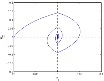
The qualitative behavior of the observation error dynamics is depicted in Figure 2.
We are in a position to establish the global asymptotic stability of the error system within the framework of methods of nonsmooth Lyapunov functions with negative semidefinite time derivative along the dynamics of the system.
Theorem 3: Let the parameters of system (12) be such that k1, k3 > 0, k2, k4 ≥ 0, and ε ≥ 0.
Then system (12) is globally asymptotically stable.
Proof: First of all, let us note that the discontinuous system (12), being viewed in the sense
−0.1 −0.05 0 0.05 0.1 −0.2 −0.15 −0.1 −0.05 0 0.05 0.1 0.15 0.2 e 1 e 2
Fig. 2. Phase trajectory of the observation error system (12), initialized with e1(0) = −0.1, e2(0) = 0 and specified with
k1= 0.1, k2= 0.2, k3= 0.1, k4= 1, and ε = 12.
condition
e1˙e1 = e1(e2− k1|e1|εsign e1− k2e1) < 0
for sliding modes to exist holds for all infinitesimal e1 6= 0 if and only if ε = 0 and |e2| < k1.
Thus, the sliding modes appear in system (12) just in the case of ε = 0. Now, let us consider the Lyapunov candidate function
V0(e1, e2) = k3|e1| + 1 2k4e 2 1+ 1 2e 2 2. (13)
By computing the time derivative of this function along the trajectories of system (12), we arrive at
˙
V0 = (k3sign e1+ k4e1)(e2− k1|e1|εsign e1− k2e1)
−e2(k3sign e1+ k4e1) = −k1k3|e1|ε
−k1k4|e1|ε+1− k2k3|e1| − k2k4e21 < 0 (14)
Inequality (14) subject to ε = 0 ensures that for ε = 0, the trajectories of (12) hit the sliding mode interval Ik1 = {(e1, e2)] ∈ R
2 : e
1 = 0, |e2| < k1} in finite time because otherwise they
steer to the origin in finite time. Since the sliding modes on the interval Ik1 are governed by the
asymptotically stable equation
˙e2 = −
k3
k1
e2, (15)
system (12), corresponding to ε = 0, is globally asymptotically stable.
For the convenience of the reader, recall that the sliding mode equation (15) is derived according to the equivalent control method [12] by substituting the equivalent value signeqe1
of the commuting function sign e1 (that ensures the identity ˙e1 = 0 along the sliding modes)
into the second equation of the disturbance-free system (12) for sign e1. As a matter of fact, the
equivalent value represents a solution of the algebraic equation e2− k1sign e1 = 0 with respect
to sign e1 and hence, signeqe1 = k1−1e2.
Finally, confining our demonstration to the case ε > 0 yields no sliding modes on the discontinuity manifold e1 = 0. Thus, by virtue of ε > 0, inequality (14) holds almost everywhere,
and the global asymptotic stability in this case is concluded by applying the extension of the invariance principle, made in [2, Theorem 3.2], to the discontinuous system (12). Theorem 3 is completely proved.
It should be pointed out that by straightforward inspection [2, Definition 4.6], system (12), specified with ε = 1
2, is homogeneous of degree q = −1 with respect to dilation r = (2, 1) so
that by the homogeneity principle [2, Theorem 4.2], the global finite time stability of this system is additionally guaranteed by its global asymptotic stability. Our next aim is to demonstrate that the finite time stability of system (12) persists in spite of certain perturbations of the parameter
ε around its homogeneity value ε = 1
2. For this purpose, we introduce the modified Lyapunov
function V1(e1, e2) = 2k3|e1| + k4e21+ 1 2e 2 2+ 1 2s 2(e 1, e2) (16)
square of the right hand-side
s(e1, e2) = e2− k1|e1|εsign e1− k2e1, (17)
of the first equation of (12). The proposed modification is inspired from [10] where the same Lyapunov function, being specified with ε = 1
2, has been used to prove the system finite time
stability in this particular case.
As the Lyapunov function (16) is shown to admit the estimate ˙
V1(t) ≤ −κV1ε(t) (18)
along the trajectories of system (12), specified with ε ∈ [1
2, 1), for some κ > 0 and for almost
all t ≥ 0, it plays a crucial role in establishing the finite time stability of such a system and in determining an upper bound of the settling-time function T (e0
1, e02) in terms of the initial value
v0 = V1(e1(0), e2(0)) of the Lyapunov function (16) and the function
γ = min ½ 2k1k3 4k3+ 3k21 ,εk1 2 , 2k1k4 2k4+ 3(k12+ k22) ¾ (19) of the system parameters. Recall that the settling-time function
T (e01, e02) = inf {T ≥ 0 : e1(t, e01) = e2(t, e02) = 0 for all t ≥ T } (20)
is defined for a solution e1(t, e01), e2(t, e02) of (12), initialized with e1(0) = e01, e2(0) = e02. The
following result is in order.
Theorem 4: Given positive k1, k2, k3, k4, and ε ∈ [12, 1), system (12) is globally finite time
stable, and an upper estimate
T (e01, e02) ≤ v1−ε0 (1 − ε)−1κ−1 (21) of the settling-time function holds for the initial value v0 of the Lyapunov function (16), for
κ = γ(2k3)1−ε, and for γ given by (19).
(12) provided that the conditions of Theorem 4 hold. Thus, the Lyapunov function (16) is almost always differentiable along the trajectories of the system in question, namely, for all t ≥ 0 such that e1(t) 6= 0. For those t, the time derivative of the Lyapunov function, computed according
to (12), proves to be negative definite. Indeed, since
|e1|ε−1 ≥ µ V1 2k3 ¶ε−1 (22) one arrives at ˙ V1 = 2sk3sign e1+ 2sk4e1− e2(k3sign e1+ k4e1) −s[εk1s|e1|ε−1+ k3sign e1+ k4e1+ k2s] = −k2s2− k1εs2|e1|ε−1− k1k4|e1|ε+1− k2k3|e1| −k2k4e21− k1k3|e1|ε = −|e1|ε−1[k2s2|e1|1−ε +k1εs2+ k1k4e21+ k2k3|e1|2−ε+ k2k4|e1|3−ε +k1k3|e1|] ≤ − µ V1 2k3 ¶ε−1 Wε(e1, s) (23) where Wε(e1, s) = [k2s2|e1|1−ε+ k1εs2+ k1k4e21+ k2k3|e1|2−ε+ k2k4|e1|3−ε+ k1k3|e1|]. (24)
Employing the well-known inequality 2ab ≤ a2+b2, a, b ∈ R and taking into account that under
the condition ε ∈ [1
2, 1) of the theorem, |e1|2ε ≤ |e1|2 for |e1| ≥ 1 and |e1|2ε ≤ |e1| otherwise,
the validity of the estimate
V1(e1, e2) ≤ 2k3|e1| + (k4+ 3 2k 2 2)e21+ 2s2+ 3 2k 2 1e2ε1 ≤ (2k3+ 3 2k 2 1)|e1| + (k4+ 3 2k 2 2 + 3 2k 2 1)e21+ 2s2 (25)
is then verified for all e1, e2 ∈ R and s, governed by (17). It is therefore clear that
for γ, governed by (19), and for all e1, e2, s ∈ R such that (17) holds. Thus, inequality (18) is
derived from (19), (23) – (26) with κ = γ(2k3)1−ε.
To complete the proof it remains to demonstrate that system (12) reaches the origin in finite time and the settling-time function (20) admits estimate (21). For this purpose, let us note that for an admissible ε ∈ [1
2, 1), the solution of the Cauchy problem
˙v(t) = −κvε(t), v(0) = v
0 (27)
is given by v(t) = [v1−ε0 − (1 − ε)κt]1−ε1 and it vanishes at T = v1−ε
0 (1 − ε)−1κ−1. By applying
comparison principle [13], the solutions V1(t) of the differential inequality (18), initialized with
V1(0) = v0, are upper estimated by the solution v(t) of the Cauchy problem (27), thereby
ensuring that the Lyapunov function (16), computed on the solutions of the system in question, is nullified after the same time instant T . The validity of Theorem 4 is thus concluded.
In the rest of this section, we carry out relations between the observer gains ki, i = 1, 2, 3, 4
that could ensure the robustness of the perturbed dynamics ˙e1 = e2− k1|e1|εsign e1− k2e1,
˙e2 = w − k3sign e1− k4e1. (28)
As a matter of fact, these dynamics correspond to the observation errors e = (e1, e2)T, e1 =
x − ˆx, e1 = y − ˆy between the state of the double integrator (5), affected by an admissible
external disturbance (8), and that of the velocity observer (10).
The desired relations, which are found for the admissible disturbances (8) with α = 1 − ε and
ε ∈ [1 2,
2
3], depend on the disturbance upper bound µ0 in the growth condition (8) and they are
as follows: k1 > 0, k2 > 1, k3 > max ½ µ0k1 k2 ,µ0(µ0+ k2) k1 ¾ , k4 > µ0(µ0+ k2) k2 . (29)
w(t). Let
ε ∈ [1
2, 2
3] and α = 1 − ε, (30) and let the system parameters meet condition (29). Then system (28) is globally finite time stable for any admissible disturbance (8), and the corresponding settling-time function is estimated by (21) with κ = γ1(2k3)1−ε and γ1 given by
γ1 = min ½ 2(k1k3− µ20− µ0k2 4k3+ 3k21 ,εk1 2 , 2k1k4 2k4+ 3(k21+ k22) ¾ . (31)
Proof: Differentiation (23) of the Lyapunov function (16) along the perturbed system (28)
beyond the discontinuity line e1 = 0 is readily modified to
˙
V1 = −|e1|ε−1Wε(e1, s)
+2sw + k1w|e1|εsign e1+ k2we1. (32)
By taking into account (26) and employing (8), (30), this yields ˙ V1 ≤ −|e1|ε−1Wε(e1, s) +s2+ w2+ k 1w|e1|εsign e1+ k2we1 ≤ −|e1|ε−1[Wε(e1, s) + s2|e1|1−ε+ w2|e1|1−ε +k1we1+ k2w|e1|2−ε] ≤ −|e1|ε−1[Wε(e1, s) +s2|e 1|1−ε+ µ20|e1|3−3ε+ µ0k1|e1|2−ε +µ0k2|e1|3−2ε] (33)
for all t ≥ 0 when e1(t) 6= 0. As established in the proof of Theorem 3, no sliding modes
occur on the discontinuity line e1(t) = 0. Thus, (30) holds almost for all positive t. Since
|e1|3−iε ≤ |e1|3−ε, i = 2, 3 for |e1| ≥ 1 and |e1|3−iε ≤ |e1|, i = 2, 3, otherwise, it follows that
is in force almost for all t ≥ 0 where
W1(e1, s) = [(k2− 1)s2|e1|1−ε+ k1εs2+ k1k4e21
+(k2k3− µ0k1)|e1|2−ε
+(k1k3− µ20− µ0k2)|e1|
+(k2k4− µ20− µ0k2)|e1|3−ε]. (35)
Furthermore, the estimate
W1(e1, s) ≥ γ1V1(e1, e2) (36)
similar to (26), is derived for γ1, given by (31), and for all e1, e2, s ∈ R such that (17), (29),
(30) hold. Relations (22), (33) – (36), coupled together, result in (18) with κ = γ1(2k3)1−ε. The
finite time stability of the perturbed system (28) and the corresponding settling-time function estimate are then concluded from inequality (18) by applying the same line of reasoning as that used in the proof of Theorem 4.
It is of interest to note that system (28), specified with ε = 1
2, remains finite time stable even
if affected by a non-vanishing external disturbance. For later use, we denote
γ2 = min{2(k1k3−M −M k1) 4k3+3k12 , k1−2M 4 } if x2 = x4 = 0 min{2(k1k3−M −M k1) 4k3+3k12 , k1−2M 4 ,2k2k4+3k1k422} otherwise (37)
Theorem 6: Let system (28) be specified with ε = 1
2 and let it be affected by a uniformly
bounded disturbance (6). Furthermore, let the system gains be such that
k1, k3 > 0, k2, k4 ≥ 0,
if k4 = 0 then k2 = 0. (38)
of the external disturbance w meets the condition M < min{k1 2, k1k3 1 + k1 }. (39)
In addition, the corresponding settling-time function is estimated by (21) with κ = γ2(2k3)1−ε
and γ2 given by (37).
Proof: Under the conditions of Theorem 6, differentiation (32) of the Lyapunov function
(16) along system (28) beyond the discontinuity line e1 = 0 is specified to
˙ V1 ≤ −|e1|− 1 2W ε=1 2(e1, s) + 2M|s| + Mk1|e1| 1 2 +Mk2|e1| = −|e1|− 1 2{W ε=1 2 − M[2|s||e1| 1 2 −k1|e1| − k2|e1| 3 2]} ≤ −|e1|−12W2(e1, s) (40)
where the well-known inequality 2|s||e1|
1
2 ≤ s2+ |e1| is taken into account and
W2(e1, s) = [k2s2|e1| 1 2 + (k1 2 − M)s 2+ k 1k4e21 +(k2k3− Mk2)|e1| 3 2 + (k1k3− M − Mk1)|e1|k2k4|e1| 5 2]. (41)
Since the first inequality of (25) reduces now to
V1(e1, e2) ≤ (2k3+ 3 2k 2 1)|e1| + (k4 + 3 2k 2 2)e21+ 2s2, (42) it follows that W2(e1, s) ≥ γ2V1(e1, e2) (43)
for γ2, given by (37), and for all e1, e2, s ∈ R such that relations (17), (38), (39) hold. Similar
to that of the proof of Theorem 5, relation (18) with ε = 1
2 and κ = γ2(2k3)1−ε is then derived
from (22), (40) – (43), coupled together. This completes the proof of Theorem 6 because as shown in the proof of Theorem 4, inequality (18) ensures that the Lyapunov function (16) is nullified after the finite time instant T = v1−ε
IV. FINITETIME STABILIZINGPOSITIONFEEDBACKSYNTHESIS
In this section, we proceed with the design of the position feedback, stabilizing the double integrator in finite time. For this purpose, we substitute the velocity y in the state feedback (2) by its estimate ˆy to arrive at the finite time stabilizing position feedback
u = −µ|ˆy|αsign ˆy − ν|x|2−αα sign x, (44)
so that the resulting closed-loop system proves to be globally finite time stable regardless of whichever admissible disturbance affects the system.
Theorem 7: Consider system (5) under the growth condition (8) on the external disturbance w. Let (5) be driven by the observer-based dynamic feedback (10), (44) with parameters α, ε
subject to (30), with positive controller gains µ, ν such that µ > µ0, and with observer parameters
ki, i = 1, 2, 3, 4, satisfying condition (29). Then the closed-loop system (5), (10), (44) is globally
asymptotically stable, regardless of whichever external disturbance (8) affects the system.
Proof: Clearly, the closed-loop system (5), (10), (44), rewritten in terms of the observation
error (28), meet the conditions of Theorem 5. By applying Theorem 5 to the observation error system (28), it is concluded that starting from a finite time instant T , the closed-loop system evolves on the manifold e1 = e2 = 0 where ˆy = y, thereby ensuring that the position control
signal (44) coincides with the state feedback signal (2). Due to this, the linear growth conditions
|w(x, y, t)| ≤ µ0(1 + |y|) and |u(x, ˆy)| ≤ µ(1 + |ˆy|) + ν(1 + |x|) turn out to hold for all
x, y ∈ R, t ≥ 0 and for the external disturbance (8) and the control input (44), respectively,
so that the closed-loop state cannot escape to infinity in finite time. To complete the proof it remains to apply Theorem 2 to (5), (10), (44) for t ≥ T when the position feedback equals the state feedback. The global asymptotic stability of the closed-loop system (5), (10), (44) is thus established.
To this end, we present the position feedback controller that additionally imposes on the closed-loop system global finite time stability and robustness against uniformly bounded disturbances.
Theorem 8: Let system (5) be affected by a uniformly bounded disturbance (6) and let it be
driven by the observer-based dynamic feedback (10), (44) specified with α = 0 and ε = 1 2,
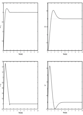
0 1 2 3 4 5 6 7 8 9 10 −2 −1.5 −1 −0.5 0 0.5 Time [sec] e 1 0 1 2 3 4 5 6 7 8 9 10 −2 −1.5 −1 −0.5 0 0.5 1 Time [sec] x 0 1 2 3 4 5 6 7 8 9 10 −0.2 0 0.2 0.4 0.6 0.8 1 1.2 1.4 1.6 Time [sec] e 2 0 1 2 3 4 5 6 7 8 9 10 −0.5 0 0.5 1 1.5 2 2.5 3 Time [sec] y
Fig. 3. Position feedback stabilization (10), (44) of the double integrator (5), initialized with x(0) = −2, y(0) = 0 and specified with µ = 1, ν = 2, α = 1
2, and ε = 1
2 .
with positive controller gains µ, ν subject to (7), and with observer parameters ki, i = 1, 2, 3, 4,
satisfying conditions (38), (39). Then the closed-loop system (5), (10), (44) is globally finite time stable.
Proof: By applying Theorem 6 to the observation error system (28), it is concluded that
starting from a finite time instant T , the closed-loop system evolves on the manifold e1 = e2 = 0
where ˆy = y, thereby ensuring that the position control signal (44) coincides with the state
feedback signal (2). Since the linear growth conditions |w(x, y, t)| ≤ M and |u(x, ˆy)| ≤ µ(1 + |ˆy|) + ν(1 + |x|) turn out to hold for all x, y ∈ R, t ≥ 0 and for the external disturbance (6) and
the control input (44), respectively, the closed-loop state cannot escape to infinity in finite time. Now applying [4, Theorem 4.2] to (5), (10), (44), provided that for t ≥ T , the position feedback equals the state feedback, yields the global finite time stability of the closed-loop system (5),
Numerical simulations, made for the double integrator (5), driven by the observer-based dynamic feedback (10), (44), are presented in Figure 3.
V. CONCLUSIONS
A modification of the twisting controller and that of the supertwisting observer are coupled together to present a unified framework for the finite time position feedback stabilization of a double integrator. The proposed modifications are shown to inherit, from their originators, desired finite time stability and robustness properties. The former modification represents a parameterized family of homogeneous continuous controllers and it is made for avoiding the undesired chattering phenomenon that appears in the closed loop if driven by a switching input of high frequency. In turn, observer switching is not as serious as controller switching because it does not drive an actuator and hence it does not come at the expense of controller switching. Therefore, the latter modification represents a parameterized family of inhomogeneous switched observers, and the motivation behind this modification is in extending the class of finite time stable SOSM’s towards their inhomogeneous perturbations.
Being coupled together, the modification of the twisting controller and that of the supertwisting observer yield the position feedback stabilization of the double integrator in finite time in accordance with the separation principle which is shown to be in force in the present case. The finite time convergence and robustness properties of the proposed synthesis make it attractive for further extension to electromechanical applications with hard-to-model nonlinear phenomena such as friction and impacts. Finite time orbital stabilization of a biped robot is among open problems to be tackled through the developed approach. This work is in progress and it will be published elsewhere.
REFERENCES
[1] S. Bhat and D. Bernstein, “Continuous finite-time stabilization of the translational and rotationnal double integrator,” IEEE
Transaction on Automatic Control, vol. 43, no. 5, pp. 678–682, 1998.
[2] Y. Orlov, Discontinuous systems – Lyapunov analysis and robust synthesis under uncertainty conditions. Springer-Verlag, London, 2009.
[3] J. W. Grizzle, J. H. Choi, H. Hammouri, and B. Morris, “On observer-based feedback stabilization of periodic orbits in bipedal locomotion,” in Proc. Methods and Models in Automation and Robotics MMAR, Szczecin, Poland, 2007. [4] Y. Orlov, “Finite-time stability and robust control synthesis of uncertain switched systems,” SIAM J Contr Optimiz, vol. 43,
[5] J. Davila, L. Fridman, and A. Levant, “Second-order sliding mode observer for mechanical systems,” IEEE Trans. on
Automatic Control, vol. 50, pp. 1785–1789, 2005.
[6] L. Fridman and A. Levant, Higher order sliding modes as a natural phenomenon in control theory. In: Garafalo F., Glielmo L. (eds) Robust control via variable structure and Lyapunov techniques. Lecture Notes in Control and Information Science, Springer, Berlin, 1996.
[7] ——, Higher order sliding modes. In: W. Perruquetti , J. P. Barbot (eds) Sliding mode control in engineering. Marcel Dekker, New York, 2002.
[8] G. Bartolini, “Chattering phenomena in discontinuous control systems,” Int. J. Syst Sci, vol. 20, pp. 2471–2481, 1989. [9] G. Bartolini, A. Ferrara, and E. Usai, “Chattering avoidance by second-order sliding mode control,” IEEE Transaction on
Automatic Control, vol. 43, pp. 241–246, 1998.
[10] J. Moreno and M. Osorio, “A lyapunov approach to second-order sliding mode controllers and observers,” in Proc. 47
IEEE Conf. on Decision and Control CDC, Cancun, Mexique, December 9–11, 2008, pp. 2856–2861.
[11] A. F. Filippov, Differential equations with discontinuous right-hand sides. [Kluwer Academic Publisher, Dordrecht, 1988. [12] V. I. Utkin, Sliding modes in control optimization. Springer-Verlag, Berlin, 1992.