UNIVERSITÉ DE MONTRÉAL
THREE DIMENSIONAL NUMERICAL PREDICTION OF ICING RELATED
POWER AND ENERGY LOSSES ON A WIND TURBINE
ECE SAGOL
DÉPARTEMENT DE GÉNIE MÉCANIQUE ÉCOLE POLYTECHNIQUE DE MONTRÉAL
THÈSE PRÉSENTÉE EN VUE DE L’OBTENTION DU DIPLÔME DE PHILOSOPHIAE DOCTOR
(GÉNIE MÉCANIQUE) AVRIL 2014
UNIVERSITÉ DE MONTRÉAL
ÉCOLE POLYTECHNIQUE DE MONTRÉAL
Cette thèse intitulée :
THREE DIMENSIONAL NUMERICAL PREDICTION OF ICING RELATED POWER AND ENERGY LOSSES ON A WIND TURBINE
présentée par : SAGOL Ece
en vue de l’obtention du diplôme de : Philosophiæ Doctor a été dûment accepté par le jury d’examen constitué de : M. CAMARERO Ricardo, Ph.D., président
M. REGGIO Marcelo, Ph.D., membre et directeur de recherche M. ILINCA Adrian, Ph.D., membre et codirecteur de recherche M. TRÉPANIER Jean-Yves, Ph.D., membre
DEDICATION
ACKNOWLEDGEMENTS
I would like to express my gratitude to my supervisor, Prof. Marcelo Reggio, and my co-supervisor, Prof. Adrian Ilinca, for their patient guidance and invaluable support throughout this study. I am also grateful to my colleagues Fernando Villalpando and Fahed Martini for answering my questions on Computational Fluid Dynamics analysis. I thank the Wind Energy Strategic Network (WESNET) for providing financial support for my study. Finally, I would like to express my great appreciation to my husband Mert Cevik for his invaluable support.
RÉSUMÉ
Plusieurs régions du Canada sont soumises à des conditions hivernales difficiles qui persistent pendant plusieurs mois. En conséquence, les éoliennes situées dans ces régions sont exposées aux effets du froid, à l'accumulation de glace et à leurs effets négatifs qui se manifestent de la perte de puissance temporaire jusqu’à l’arrêt complet de la machine. Dans certains sites au Canada, la perte de production annuelle d'une turbine éolienne peut atteindre jusqu'à 16% de sa valeur nominale et l'estimation de ces pertes avant la construction d'un parc éolien devient essentielle pour les développeurs et investisseurs.
La revue de la littérature montre que la plupart des logiciels de prévision de givrage ont été développés pour les avions, et sont, en majorité, la propriété d’entreprises et inaccessibles aux chercheurs œuvrant dans d'autres domaines. En plus, le givrage des avions est différent de celui de l'éolienne. Les éoliennes sont exposées à des conditions de givrage pour des périodes beaucoup plus longues que les avions, peut-être pour plusieurs jours dans un climat rude, alors que la durée maximale de l'exposition d'un avion est d'environ 3-4 heures. En outre, les pales d'éoliennes fonctionnent à des vitesses subsoniques, à des nombres de Reynolds inférieurs à ceux des avions, et leurs caractéristiques physiques sont différentes. Quelques logiciels ont été cependant développés pour le givrage des éoliennes. Toutefois, ils sont soit en 2D et ne considèrent pas les caractéristiques 3D du champ d'écoulement, ou se concentrent sur la simulation de chaque rotation d'une manière dépendante du temps, ce qui n'est pas pratique pour le calcul de longues heures de l'accumulation de glace.
Dans ce contexte, notre objectif dans cette thèse est de développer une méthodologie numérique 3D pour prédire la forme de givre et la perte de puissance d'une éolienne en fonction des conditions météorologiques. En plus, nous calculons la production énergétique annuelle d'une turbine typique pour des conditions normales d’exploitation et en tenant compte des évènements givrants. Les calculs sont effectués en utilisant une éolienne pour laquelle des nombreuses données sont disponibles, l'éolienne NREL Phase VI et les conditions météorologiques d'un parc éolien en Suède pour lequel les évènements de givrage sont enregistrés et publiés.
La méthode proposée est basée sur le calcul et la validation de la performance de l'éolienne propre, le calcul de la forme de givre et de la performance de la pale givré, pour des conditions de givrage typiques. La première étape consiste à calculer la performance du NREL Phase VI en
utilisant un outil CFD commercial, ANSYS-FLUIDES. Afin de réduire le coût de calcul, on utilise un modèle de rotation du domaine de référence de la pale avec un calcul des valeurs temporelles moyennes des propriétés de l'écoulement. Une étude de la sensibilité du maillage a permis de déterminer sa taille optimale du maillage afin de respecter les conditions de convergence et de précision. Parmi les modèles de turbulence existants, nous avons sélectionné
SST k-ω qui a fourni les meilleurs résultats pour les conditions d’écoulement autour de pales
givrées, caractérisées par des larges zones de décrochage. En général, les coefficients de pression et le moment de flexion concordent bien avec les données expérimentales, en particulier pour des vitesses avant le décrochage. Bien que le couple prédit s'écarte des données expérimentales, la tendance de variation par rapport à la vitesse du vent est similaire.
Après que la courbe de puissance de la pale propre est calculée, nous déterminons l'efficacité de collection qui caractérise la masse d’eau surfondue qui frappe la pale et qui est directement proportionnelle au taux de givrage d'une surface. Une analyse multiphasique pour les phases d'air et d'eau (approche eulérienne) est utilisée pour calculer le taux d'accumulation des gouttelettes sur la surface de la pale. Les deux approches permettant de caractériser l’écoulement des gouttelettes d’eau, eulérienne et lagrangienne, ont été étudiées avant de décider laquelle était la plus appropriée pour notre étude. La première méthode (eulérienne) est caractérisée par la résolution des équations de mouvement de toute la phase liquide, tandis que la seconde méthode (lagrangienne) est basée sur le calcul de la trajectoire de chaque gouttelette dans l'air. Nous avons finalement choisi le modèle Eulérien pour notre étude, car il peut être adapté pour traiter les maillages vastes et complexes mieux que le modèle Lagrangien. La validation de cette étape est exécutée sur un profil aérodynamique, NACA 0012, comme des données expérimentales en 3D ne sont pas disponibles.
Ensuite, l'accumulation de glace sur l'éolienne est calculée en utilisant des méthodes « Quasi-3D » et « Fully-Quasi-3D », basées sur des modèles physiques similaires, mais avec une considération différente des aspects tridimensionnels. Pour la méthode Quasi-3D, toutes les étapes mentionnées sont réalisées en 2D et la puissance totale est calculée en utilisant la méthode "Blade Element Momentum ", alors que le « Fully-3D » effectue toutes les étapes dans un domaine 3D. La méthode « Fully-3D » donne des prévisions de la puissance plus précises pour la pale propre. Pour la pale givrée, la validation a été impossible en raison du manque de données expérimentales et de résultats d’autres modélisations. Cependant, les deux méthodes donnent des
résultats différents pour la forme de la glace et pour la performance de la pale givrée. Une analyse critique des résultats montre que, bien que le coût de calcul de la méthode entièrement 3D est beaucoup plus élevé, la prédiction du givrage en 2D peut manquer de précision, la forme de la glace et la perte de puissance sont surestimées en raison de l'absence des effets 3D de l’écoulement de rotation.
En effectuant les calculs CFD sur la pale givrée, la surface rugueuse du givre est lissée jusqu'à un certain niveau pour éviter l'instabilité numérique et pour garder un nombre raisonnable d’éléments de maillage. Cependant, l'effet de la rugosité ne peut être exclu, car il contribue de façon significative à la diminution de la performance. Pour cette raison, la présence de la rugosité de la glace est prise en compte par une modification dans le code CFD. L'effet de la rugosité sur la performance est analysé aussi sur la pale propre.
Enfin, la production annuelle d'énergie de l'éolienne est calculée pour un parc éolien pour lequel les conditions de givrage sont disponibles dans la littérature. Des analyses paramétriques des valeurs du contenu en eau liquide et la taille des gouttelettes montrent comment ces paramètres affectent la forme de glace et les performances des turbines éoliennes. Par ailleurs, les productions énergétiques annuelles pour les configurations propre et givrée sont comparées.
ABSTRACT
Regions of Canada experience harsh winter conditions that may persist for several months. Consequently, wind turbines located in these regions are exposed to ice accretion and its adverse effects, from loss of power to ceasing to function altogether. Since the weather-related annual energy production loss of a turbine may be as high as 16% of the nominal production for Canada, estimating these losses before the construction of a wind farm is essential for investors.
A literature survey shows that most icing prediction methods and codes are developed for aircraft, and, as this information is mostly considered corporate intellectual property, it is not accessible to researchers in other domains. Moreover, aircraft icing is quite different from wind turbine icing. Wind turbines are exposed to icing conditions for much longer periods than aircraft, perhaps for several days in a harsh climate, whereas the maximum length of exposure of an aircraft is about 3-4 hours. In addition, wind turbine blades operate at subsonic speeds, at lower Reynolds numbers than aircraft, and their physical characteristics are different. A few icing codes have been developed for wind turbine icing nevertheless. However, they are either in 2D, which does not consider the 3D characteristics of the flow field, or they focus on simulating each rotation in a time-dependent manner, which is not practical for computing long hours of ice accretion.
Our objective in this thesis is to develop a 3D numerical methodology to predict rime ice shape and the power loss of a wind turbine as a function of wind farm icing conditions. In addition, we compute the Annual Energy Production of a sample turbine under both clean and icing conditions. The sample turbine we have selected is the NREL Phase VI experimental wind turbine installed on a wind farm in Sweden, the icing events at which have been recorded and published.
The proposed method is based on computing and validating the clean performance of the turbine, and then computing the ice shape and iced blade performance, under icing conditions. The first step is to compute the performance of the NREL Phase VI using the commercial ANSYS-FLUENT computational fluid dynamics (CFD) tool. In order to reduce the computational cost, we use a rotating reference frame model which computes the flow properties as time-averaged quantities. A grid sensitivity study has been performed to eliminate the effect of mesh on the
results. Of the existing models for characterizing turbulence, we have selected the two-equation
SST k-ω model. In general, the computed pressure coefficients and bending moment have shown
good agreement with the experimental data, particularly at pre-stall speeds. Although the torque deviates from the experimental data, the trend with respect to the wind speed is similar.
After the clean power curve has been computed, collection efficiency, which is directly proportional to the rate of icing of a surface, is analyzed. A multiphase analysis, for the air and water phases, is necessary to compute the rate of accumulation of the droplets on the blade surfaces. We study two different approaches that are found in the literature – Eulerian and Lagrangian – and determine the most suitable one for our study case. The former applies the governing equations to the liquid phase, while the latter computes the trajectory of each droplet present in the air. We eventually decided on the Eulerian model for our study, as it can be adapted to handle large and complex meshes better than the Lagrangian model. This step is validated on a NACA 0012 airfoil, as experimental data for 3D flows are not available in the literature.
The ice accretion on the sample wind turbine blades is computed using both a Quasi-3D and a Fully-3D method, which have a similar theoretical background, but a different order of modeling. In the former, all the steps are carried out in 2D and the overall power is computed using the Blade Element Momentum method, while the latter performs all the steps in the 3D domain. The Fully-3D method yields more accurate predictions for a clean blade. For icing conditions, a validation is not possible, owing to the lack of experimental data. However, the two methods produce quite different results for the performance of the ice shape and the iced blade. A critical analysis of the results shows that, although the computational cost of the Fully-3D method is much higher, icing analyses in 2D may lack accuracy, because the ice shape and the related power loss are compromised by not considering the 3D features of rotational flow.
While performing the CFD computations on the iced blade, the rough surface of the ice is smoothed to a degree, in order to prevent numerical instability and to keep the mesh size within a reasonable limit. However, roughness effects cannot be excluded altogether, as they contribute significantly to performance reduction. We consider roughness through a modification in the CFD code, and assess its effect on performance for the clean blade.
Finally, the Annual Energy Production of the wind turbine is computed for a selected wind farm, the icing conditions of which are available in the literature. Parametric analyses of Liquid Water Content and the droplet size reveal how the variation of these parameters affects the ice shape and performance of the turbine. We also compared the energy production of clean and iced blade configurations.
TABLE OF CONTENT
DEDICATION ... III ACKNOWLEDGEMENTS ... IV RÉSUMÉ ... V ABSTRACT ... VIII TABLE OF CONTENT ... XI LIST OF TABLES ... XV LIST OF FIGURES ... XVI LIST OF ABBREVIATIONS ... XX LIST OF APPENDICES ... XXIIINTRODUCTION ... 1
Description of the Problem ... 1
Objectives ... 6
Organization of the thesis ... 7
Chapter 1 CRITICAL REVIEW ... 10
1.1 CFD Analysis of a Wind Turbine Rotor ... 11
1.2 Wind Tunnel & On-Site Experiments on Icing ... 13
1.3 Numerical Investigation of Icing ... 15
1.3.1 Collection Efficiency Analysis ... 15
1.3.2 Ice Shape Computation ... 17
1.4 Iced Airfoil & Blade Aerodynamics ... 21
Chapter 2 METHODOLOGY ... 24
2.2 Phase II – Collection Efficiency Analysis ... 24
2.3 Phase III – Ice Accretion Computation ... 31
2.4 Phase IV – Iced Blade Analysis ... 34
2.5 Phase V – Power and Energy Loss Modeling ... 35
Chapter 3 ARTICLE 1: ISSUES CONCERNING ROUGHNESS ON WIND TURBINE BLADES... ... 38
3.1 Abstract ... 38
3.2 Introduction ... 38
3.3 Surface Roughness and Its Sources ... 39
3.3.1 Dust accumulation ... 39
3.3.2 Insect contamination ... 40
3.3.3 Ice Accumulation ... 41
3.3.4 Other Roughness Sources ... 41
3.3.5 Characterization of Roughness ... 42
3.4 Effects of roughness on flow field ... 42
3.5 Effects of Roughness on Performance ... 44
3.6 Numerical efforts for modeling roughness ... 47
3.7 Solutions to the roughness problem ... 49
3.7.1 Specially designed airfoils ... 49
3.7.2 External Solutions ... 51
3.8 Concluding Remarks ... 52
Chapter 4 ARTICLE 2: ASSESSMENT OF TWO-EQUATION TURBULENCE MODELS AND VALIDATION OF THE PERFORMANCE CHARACTERISTICS OF AN EXPERIMENTAL WIND TURBINE BY CFD ... 67
4.2 Introduction ... 68 4.3 Methodology ... 70 4.3.1 Experimental Data ... 70 4.3.2 Numerical Set-Up ... 71 4.4 Results ... 76 4.4.1 Grid Convergence ... 76
4.4.2 Comparison of Turbulence Models. ... 77
4.4.3 Comparison of Moments on the Blade. ... 78
4.5 Concluding Remarks ... 79
4.6 Acknowledgment ... 80
Chapter 5 ARTICLE 3: COMPARISON OF THE QUASI-3D AND FULLY 3D METHODS FOR MODELING WIND TURBINE ICING ... 87
5.1 Abstract ... 87 5.2 Introduction ... 87 5.3 Methodology ... 90 5.3.1 Quasi-3D (Q3D) Method ... 91 5.3.2 Fully 3D (F3D) Method ... 93 5.3.3 Test Case ... 94
5.3.4 Numerical Scheme and Mesh Characteristics ... 94
5.4 Results ... 95
5.4.1 Clean Blade Analysis ... 95
5.4.2 Blade Icing Analysis ... 96
5.5 Conclusion ... 97
Chapter 6 ARTICLE 4: NUMERICAL EVALUATION OF THE ROUGHNESS EFFECT ON
WIND TURBINE PERFORMANCE ... 104
6.1 Abstract ... 104
6.2 Introduction ... 105
6.3 Methodology ... 107
6.3.1 Test Case ... 107
6.3.2 Numerical Scheme and Mesh Characteristics ... 107
6.4 Results and Discussion ... 110
6.5 Conclusion ... 112
Chapter 7 SAMPLE POWER AND AEP LOSS ANALYSES ... 120
7.1 Parametric Analysis ... 122
7.2 Annual Energy Production (AEP) Loss ... 125
Chapter 8 GENERAL DISCUSSION AND CONCLUSION ... 130
8.1 Summary of the Work ... 130
8.2 Limitations of the proposed method ... 131
8.3 Future study ... 132
BIBLIOGRAPHY ... 134
LIST OF TABLES
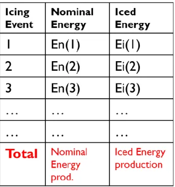
Table 2-1 Icing events for a wind farm and corresponding energy production. ... 37
Table 3-1Roughness values of surface finish applications. Reproduced from (Pechlivanoglou, 2010) ... 65
Table 3-2 Comparison of wind turbine airfoils with vortex generators. (van Rooij & Timmer, 2003) ... 66
Table 4-1 NREL phase VI experimental wind turbine characteristics ... 86
Table 5-1Characteristics of the NREL Phase VI experimental wind turbine. ... 103
Table 6-1NREL phase VI experimental wind turbine characteristics. ... 117
Table 6-2 The power loss of wind turbine compared to its clean state and estimated roughness threshold values ... 118
Table 6-3 The scenarios of AEP analyses ... 118
Table 6-4 The minimum and maximum AEP loss depending on roughness size ... 119
Table 7-1 Liquid Water Content and Droplet concentration values for the selected wind site ... 121
Table 7-2 Test matrix ... 122
Table 7-3 The power production losses due to icing of 3 to 72 hours ... 127
Table A. 1 Icing events of the sample wind farm in Blaiken, Sweden. (Carlsson, 2009)...144
LIST OF FIGURES
Figure 0-1 Classification of ice types (Bragg, Broeren, & Blumenthal, 2005) ... 3
Figure 0-2 (a) rime ice; and (b) glaze ice. (Bragg, Broeren, & Blumenthal, 2005) ... 4
Figure 0-3 In-site power measurement for an iced rotor blade and a clean rotor blade (Botta, Cavaliere, & Holttinten, 1998) ... 5
Figure 1-1 S809 performance under clean and iced conditions (Jasinski, et al. 1997) ... 14
Figure 1-2 Lift and drag coefficient change with glaze and rime icing respectively. Hochart et al. (2008) ... 15
Figure 1-3 Comparison of collision efficiencies for single-size approximation methods and spectral weighted analysis. (Finstad, Lozowski and Makkonen 1988) ... 16
Figure 1-4 Collection efficiency comparison for the NACA 0012 (Silveria, et al. 2003) ... 17
Figure 1-5 Effect of temperature on ice shape calculation (Homola, et al. 2010) ... 20
Figure 1-6 Effect of droplet size on ice shape computation (Homola, et al. 2010) ... 20
Figure 1-7 Flow separation over horn ice for the NACA 0012. (Bragg, Broeren and Blumenthal 2005) ... 22
Figure 1-8 Lift Coefficient for clean and horn-iced airfoils (Bragg, Broeren and Blumenthal 2005). ... 23
Figure 1-9 Lift and pitching moment coefficients for clean and streamwise iced airfoils (Bragg, Broeren and Blumenthal 2005) ... 23
Figure 2-1 Comparison of collection efficiency with experimental data ... 29
Figure 2-2 Collection efficiency variation with droplet size ... 30
Figure 2-3 Representative node and ice growth in neighbour cells ... 33
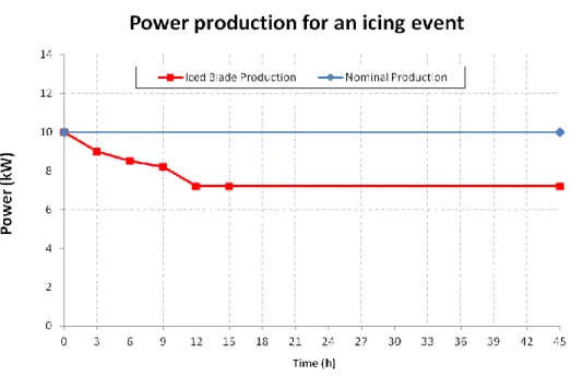
Figure 2-4 Power production during an icing event and nominal production ... 36
Figure 3-1 Rough surfaces of wind turbine blades caused by insects, ice, and erosion, respectively. (KellyAerospace) (Weiss) (BladeSmart) ... 53
Figure 3-3 Classification of ice accumulation types (Bragg, Broeren, & Blumenthal, 2005) ... 54 Figure 3-4Transition from laminar to turbulent flow. Reproduced from (Schlichting, 1979) ... 54 Figure 3-5Boundary layer transition and turbulence intensity: (a) on a smooth surface; and (b) on
a rough surface. (Turner, Hubbe-Walker, & Bayley, 2000) ... 55 Figure 3-6 Transition over the surface of a NACA 0012 for various Reynolds numbers. (Kerho &
Bragg, 1997) ... 55 Figure 3-7 Turbulence intensity level for a clean and a rough NACA 0012. (Bragg, Broeren, &
Blumenthal, 2005) ... 56 Figure 3-8 Lift and drag coefficient curves for clean and rough configurations. (Ferrer &
Munduate, 2009) ... 56 Figure 3-9 (a) Lift; and (b) drag coefficient curves for clean surfaces and surfaces with roughness
applied. (Busch, 2009) ... 57 Figure 3-10 Effect of various roughness configurations on a wind turbine blade. (Freudenreich,
Kalser, Schaffarczyk, Winkler, & Stalh, 2007) ... 57 Figure 3-11(a) Lift coefficients of clean and rough members of the NACA 64-x18 airfoil family;
and (b) drag vs. lift coefficients of clean and rough members of the NACA. (Timmer, 2009) ... 58 Figure 3-12 Effect of roughness height on the lift and drag coefficients. Reproduced from (Li, Li,
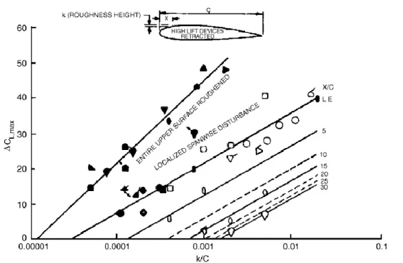
Yang, & Wang, 2010) ... 59 Figure 3-13 Effect of roughness size and location on the lift coefficient. (Bragg, Broeren, &
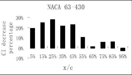
Blumenthal, 2005) ... 59 Figure 3-14 Percentage of lift coefficient decrease for different roughness. Reproduced from (Ren
& Ou, 2009) ... 60 Figure 3-15 Power production over varying operational times. (Corten & Veldkamp, 2001) ... 60 Figure 3-16 Lift and drag curve estimation over varying operational periods. (Ren & Ou, 2009) 61 Figure 3-17 Lift coefficient curve comparison: (a) Spalart–Allmaras model; and (b) k–o SST
Figure 3-18 Lift coefficient curve of an S814 airfoil from various analyses. (Ferrer & Munduate,
2009) ... 62
Figure 3-19 Lift and drag coefficients for various roughness heights. (Ren & Ou, 2009) ... 62
Figure 3-20 Comparison of wind turbine airfoils for clean and dirty configurations. (Tangler, Smith, & Jager, 1992) ... 63
Figure 3-21 Design requirements and objectives for design optimization on the lift. Reproduced from (Fuglsang, Bak, Gaunaa, & Antoniou, 2004) ... 63
Figure 3-22 Lift coefficient and lift-to-drag ratio for: (a) clean; and (b) rough configurations. (van Rooij & Timmer, 2003) ... 64
Figure 4-1(a) Twist distribution; (b) chord distribution of NREL Phase VI blade. ... 80
Figure 4-2 3D CAD model of the NREL phase VI wind turbine. ... 81
Figure 4-3 Computational domain for the NREL Phase VI rotor ... 81
Figure 4-4 (a) Surface triangular mesh, (b) domain tetrahedral and prism mesh. ... 81
Figure 4-5 Surface mesh on the tip of the blade for a coarse, amedium, and a fine grid. ... 82
Figure 4-6 Pressure coefficient comparison for various grid sizes for: a) root; b) mid-span; and c) blade tip. ... 82
Figure 4-7 Comparison of pressure coefficients for various turbulence models against experimental data for: a) root; b) mid-span; and c) blade tip ... 83
Figure 4-8 Comparison of experimental data and CFD results for (a) low-speed shaft torque; (b) root flap bending moment. ... 83
Figure 4-9 Streamlines over the blade and relative velocity distribution at 0.3R, 0.466R, 0.633R, 0.8R, and 0.95R. ... 84
Figure 4-10 Pressure coefficient comparison at stall speed, 10m/s, for: (a) 0.3R, (b) 0.466R, (c) 0.633R, (d) 0.8R, and (e) 0.95R. ... 85
Figure 5-1 Flowchart of ice accretion and performance modeling. ... 98
Figure 5-3 (a) Twist distribution; (b) chord distribution for the NREL VI blade. ... 99
Figure 5-4 Computational domains for 2D and 3D analysis. ... 100
Figure 5-5 Lift and drag coefficients computed at each section. ... 100
Figure 5-6 Total torque of a clean wind turbine from the root to the tip of the blades. ... 100
Figure 5-7(a)-(h) Ice shapes computed during 60 minutes of precipitation. ... 101
Figure 5-8 Comparison of total torque for clean and iced wind turbine blades for: (a) the Q3D method; and (b) the F3D method. ... 102
Figure 5-9 Computational time for ice accretion for the Q3D and F3D methods. ... 103
Figure 6-1(a) Twist distribution; (b) chord distribution for NREL VI blade ... 114
Figure 6-2 Computational domain with boundary conditions ... 114
Figure 6-3 The computed torque for a range of roughness values for 7m/s, 10m/s, and 15m/s .. 115
Figure 6-4 Turbulent intensity values on the blade at 10m/s wind speed ... 115
Figure 6-5 Total blade torque vs. wind speed for various roughness heights. ... 116
Figure 6-6 AEP for Scenarios 1-3 for the medium wind speed, 7m/s. ... 117
Figure 7-1 Ice shape variation for Sim1, Sim2 and Sim3 ... 123
Figure 7-2 Power curve variation for clean blade and Sim1, Sim2, and Sim3 ... 123
Figure 7-3 Ice shape variation for Sim2, Sim4, and Sim5 ... 124
Figure 7-4 Power curve variation for clean blade and Sim2, Sim4, and Sim5 ... 125
Figure 7-5 3D ice shapes computed up to 72 hours of icing ... 126
Figure 7-6 Ice growth with time for a) tip, b)mid-span, and c) root of the blade ... 126
Figure 7-7 Power curve variation for ice accretion simulation through the time. ... 127
Figure 7-8 Comparison of power loss due to icing for various wind speeds ... 128
LIST OF ABBREVIATIONS
AEP Annual Energy Production, MWh ice layer thickness, m
drag coefficient pressure coefficient
, specific heat of ice and water, J/kgK
mean diameter,
water droplet diameter, m
energy produced by clean and iced blade, kWh
water vapor pressure at altitude 1
drag function
wind Weibull function
gravity,
water layer thickness, m
k wind shape parameter
K interphase exchange coefficient latent heat from fusion, J/kg
LWC liquid water content, g/
ice mass on blade, kg
median volume diameter,
N approximate number of droplets in air
p pressure, kPa
water droplet Reynolds number
time, s
ice temperature. K
volume of ice,
velocity vector of air and water, m/s freestream velocity, m/s
volume fraction of phase q collection efficiency
the constant ratio of the molecular weight for water vapor and dry air thermal conductivity of ice and water, W/mK
shear stress component water temperature, K
LIST OF APPENDICES
APPENDIX A – COLLECTION EFFICIENCY VALIDATION ... 142 APPENDIX B – WIND FARM DATA ... 145
INTRODUCTION
Description of the Problem
The demand for more energy grows year after year, to keep pace with the increasing population of the world. Although fossil fuels are still the most widely used and widely available energy resource, they cannot meet all the energy requirements of the people on this planet, nor are they distributed evenly over the planet. As a result, fossil fuel prices frequently become unstable, as a result of production and supply crises, and countries lacking their own oil supply have been seeking alternative energy resources that are both feasible and sustainable. Another challenge is the threat of increased amounts of harmful greenhouse gases in the atmosphere due to the burning of fossil fuels, which adds to the pressure to use renewable energy resources. The Kyoto Protocol, which is aimed at reducing this greenhouse gas accumulation, has been accepted by many countries, and resulted in national and international agreements to limit the use of fossil fuels. Among the renewable energy resources being considered is wind energy, which has garnered attention because of its global availability and because it is cheap.
A number of countries, like Canada, experience long, cold winters, and wind turbines in these countries are exposed to icing, which has several adverse effects, on both the performance and the life expectancy of the turbine. Therefore, predicting energy losses due to icing is a vital issue for investors to consider.
The severity of these adverse effects will vary, depending on the amount of ice accreted. One of the most serious problems is a heavy ice load, which causes significant energy loss, as it can result in the turbine stopping altogether. Even light icing conditions are reported to cause the aerodynamic profile of the turbine blades to change and surface roughness to increase, which increases drag and decreases the lift coefficient. The article referenced in Chapter 3 provides a thorough review not only of the effects of roughness due to light icing, but also the effects of other types of contamination on wind turbine blades. In harsh winter conditions, the annual loss of power generated is reported to be as high as 16% of the nominal production for Canada (Lacroix 2013). Paradoxically, most of the numerical analyses, experiments, and wind farm measurements show that ice accretion on blades may cause a temporary increase in power generation due to delayed stalling. While this may seem to be an advantage, the wind turbine
blades are, in fact, overloaded with ice, which threatens the integrity of both the generator and the structure itself.
Icing also has an adverse effect on the structure, as it causes the blades to fatigue more quickly, with a corresponding decrease in their life expectancy. Furthermore, a non axisymmetric distribution of these loads produces edgewise vibrations, leading to the possibility of resonance (Hansen, et al. 2006). Finally, the accumulated ice on the blade may shed, propelled by rotational force, which poses a danger to residential areas, public roads, power lines, etc. located around the wind turbines.
In broad terms, icing may refer to ice accretion on structures owing to either atmospheric icing, caused by micro-sized supercooled water droplets that exist in liquid form in sub zero temperatures, or any type of precipitation, like rain or snow, accumulating on the blade in the form of ice. In this study, we refer to ice accretion on wind turbine blades caused by atmospheric icing, which typically forms in harsh winter environments and at higher altitudes.
It is important that we provide a classification of ice types before evaluating the effects of icing on wind turbines. A study by Bragg et al. (2005) classifies the ice formations according to their shapes and their influence on performance, as shown in Figure 0-1. They define the roughness type icing as the initial stages of icing, where the ice particles create small perturbations on the airfoil surface. This type of icing is reviewed in Chapter 3, and its effect on the sample wind turbine is analyzed in Chapter 6. Streamwise ice, or rime icing, follows the contours of the airfoil. Horn ice, or glaze ice, is an ice formation with a horn shape at the leading edge, as the name implies. Finally, ridge ice is made up of relatively large chunks of ice that are located separately on the airfoil. This type of icing is associated with supercooled large droplets (SLD).
Figure 0-1 Classification of ice types (Bragg, Broeren, & Blumenthal, 2005)
The types of icing that occur most frequently are glaze (horn) and rime (streamwise) icing, and these are illustrated in Figure 0-2.Glaze forms near 0oC, and a water layer covers the ice layer in this case. For this reason, it is transparent and homogeneous. It has a higher density than rime icing. The horn shape is formed by ‘runback’ water, which does not freeze at the leading edge, but later on. Glaze ice causes huge performance losses, since the horn-like structure on the upper surface causes flow separation, even at smaller angles of attack. Fortunately, this type of icing is less frequent than rime icing in cold regions.
Rime icing occurs when supercooled water droplets freeze immediately upon contact with a surface. It has a rough, opaque appearance. However, the structure follows the streamlines, and so its effect on aerodynamic flow is less destructive than that of glaze icing.
Figure 0-2 (a) rime ice; and (b) glaze ice. (Bragg, Broeren, & Blumenthal, 2005)
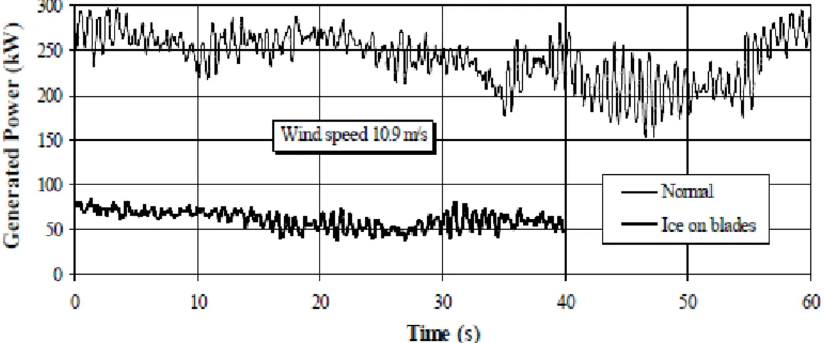
During icing events, significant losses in power production are observed in wind farm measurements. The power performance of a 400 kW iced turbine and a clean wind turbine in Italy were compared by Botta et al. (Botta, Cavaliere and Holttinten 1998) –see Figure 0-3.One minute of power measurement shows that the power of the iced turbine is about 30% that of the clean turbine. There are many examples in the literature that demonstrate the overall reduction in both power and energy production of wind turbines. Lacroix (2013) has indicated that the annual energy production losses in the Canadian provinces varies from 3% to 16%. The AEP loss measured in Quebec for the reference year was 7.4%.
Figure 0-3 In-site power measurement for an iced rotor blade and a clean rotor blade (Botta, Cavaliere, & Holttinten, 1998)
A number of icing codes are available for aircraft and wind turbines. LEWICE, developed by NASA’s Glenn Research Center, is an ice growth prediction code for aircraft. LEWICE is made up of four main modules for the computation of flow field, particle trajectory, mass, and energy balance equations, and of the updated ice shape. The flow field is computed using the panel method, which yields accurate results for fixed wing aircraft, but this prediction code has not been applied to wind turbines.
Makkonen et al. (2001) present a 2D icing code, TURBICE, to simulate glaze and rime icing on wind turbines. TURBICE also uses the panel method for flow field prediction. Comparison with experimental data shows that the shape of rime ice is predicted quite well, whereas the shape of glaze ice is not. The authors conclude that non matching ice shape measurements are a result of error in determining whether the ice growth is rime ice or glaze ice.
A comprehensive methodology for the simulation of icing on various machines is presented by Aliaga et al. (2010). FENSAP-ICE-Unsteady has the ability to predict ice shapes on aircraft and jet engines using 3D Unsteady Navier-Stokes equations for the flow field (FENSAP module), and the Eulerian method for the water droplet trajectory analysis. Although FENSAP-ICE-Unsteady is superior in terms of computing unsteady impingement on a surface, it is not cost-effective, since 2100 rotations of the rotor are needed for 1 minute of icing simulation for a helicopter. There are other codes in the literature; however the methodologies on which they are based are similar. Among these codes is CANICE (Bombardier Aerospace), TAICE (Turkey), CIRAMIL
(Italy), ONERA (France), and ICECREMO and DRA (United Kingdom). All these programs were developed for aerospace applications, i.e. aircraft icing.
To summarize, a survey of the technical literature shows that ice prediction methods are widely available for aircraft icing. However, these are commercial codes, developed specifically for aircraft industry specifications. Moreover, wind turbines are exposed to icing for longer periods than aircraft. The typical maximum icing duration for an aircraft is about 3-4 hours, whereas a wind turbine operating in a harsh winter climate may be exposed to icing for several days. Clearly, a computational method specifically developed for wind turbines is required, if we are to be able to accurately predict icing effects on these machines. A few modeling initiatives have been undertaken for ice accretion on wind turbines. However, these codes – TURBICE, FENSAP-ICE, and CIRAMIL – are either in 2D, which doesn’t take in account the 3D characteristics of the flow field, or they are commercial.
Objectives
The main objective of this thesis is to develop a 3D numerical methodology for the computation of the shape of rime ice on turbine blades and the power loss of the machine as a function of wind farm icing conditions. With this information, we can compute the corresponding annual energy loss, which is a critical parameter in wind farm construction. We perform the numerical computations using the current version of ANSYS FLUENT, and develop an in-house code for 3D rime ice prediction on the MATLAB platform.
The issues addressed to develop a 3D numerical energy loss modeling tool for iced wind turbines are as follows:
1- Computation of the flow field, calibration of CFD analysis parameters, like a turbulence model and mesh settings, and validation of the performance of the sample wind turbine blades in 3D.
2- Calculation of collection efficiency using the Eulerian multiphase model, and validation of this parameter for a sample NACA 0012 airfoil, the experimental data for which are available in the literature.
4- Computation of the flow field and performance of an iced wind turbine using the CFD tool.
5- Comparison of a 2D analysis and a 3D analysis with respect to ice shape and the corresponding performance characteristics.
6- Analysis of the wind turbine installed in a sample wind farm and computation of its annual energy loss.
7- Provide a baseline analysis method for 3D ice prediction that can be further developed for glaze icing.
3D numerical computations can predict the shape of the ice that has accumulated on blades, and the related power and energy loss of a wind turbine, as functions of wind farm icing characteristics. Additional computational resources will contribute to better prediction of the effects of icing.
3D numerical modeling has not been used to predict power curves and energy losses as a function of environmental conditions. The proposed method for estimating energy losses and ice shape is essential to the exploitation of wind turbines in cold environments.
Organization of the thesis
Along with the general organization of this thesis, we discuss the consistency of the four submitted-two of them published-papers, on this topic, and their objectives. These four journal articles are each discussed in detail in a separate chapter, and our final results are presented in a chapter following the articles.
Critical review section provides the summary and analyses of the effect of icing on wind turbines and efforts on the numerical modeling of icing. The methodology section provides a step-by-step presentation of the approach we followed to achieve our general objectives. The overall method is divided to five phases, each of which has its own specific objectives. A phase of the method is validated if experimental data are available in the literature.
The first article, “ARTICLE 1: Issues concerning roughness on wind turbine blades,” published in Renewable & Sustainable Energy Reviews of Elsevier in 2013, is presented in Chapter 3. In it, the effects on the flow field and on power generation of surface roughness caused by
contamination are reviewed, the aim being to stress that even the early stages of icing must be taken into account in the power loss computations. Although this article is not the first to have been published, we present it first, as it is a literature review.
The second article, “ ARTICLE 2: Assessment of Two-Equation Turbulence Models and Validation of the Performance Characteristics of an Experimental Wind Turbine by CFD,” was published in ISRN Mechanical Engineering in 2012. This article, which is the subject of Chapter 4, addresses the objectives of computing and validating the power performance of a clean turbine using the CFD method. In it, an appropriate turbulence model is selected by comparing the results obtained with the experimental data using various models.
The third article, “ARTICLE 3: Comparison of the Quasi-3D and Fully 3D methods for modeling wind turbine icing,” was submitted to the Journal of Wind Energy of Hindawi in March 2014. This work, Chapter 5, compares two computational approaches to calculating rime ice shape and the corresponding power loss of a wind turbine. In the first method, Quasi-3D, the collection efficiency and ice accretion shape are calculated on a number of 2D profiles of the blade, and the power curve is determined using the Blade Element Momentum method. A multiphase analysis is performed using the Eulerian approach, and the aerodynamic coefficients required for the BEM method are derived from single phase CFD simulations on the iced blade sections. In the second method, the Fully-3D method, all the calculations are executed in a 3D domain. The purpose of this comparison is to determine whether or not the additional computer resources required for the simulations in the Fully-3D method are justified by the improvement in the accuracy of the results.
The final paper, “ARTICLE 4: Numerical Evaluation of THE Roughness Effect on Wind Turbine Performance,” was submitted to the Journal of Wind Engineering and Industrial Aerodynamics in October 2013. This manuscript, the subject of Chapter 6, covers the application of a roughness model to prove the findings presented in the review article presented in Chapter 3. In this study, turbine performance is computed in the presence of roughness. Various parameters, such as the effect of wind speed, roughness size, and roughness duration, are evaluated. In addition, a simple Annual Energy Loss (AEP) study is performed for a sample wind farm, and various icing duration scenarios are presented to quantify their effect.
In the final results section, the entire methodology is applied to a specific icing case on a wind farm. The experimental data are derived from a study that measures icing duration, air temperature and humidity, and the power loss of the turbine, which is installed on a wind farm in Sweden. The ice accretion is computed from the minimum to the maximum icing duration within a certain time interval. The power loss is compared to the wind farm data for each icing event. The power curves are presented as functions of icing duration and wind speed. The Annual Energy Production is computed for both nominal and icing conditions, and the figures are compared.
Chapter 1 CRITICAL REVIEW
Ice accretion on wind turbine blades is an impediment to efficient operation in a number of ways, such as reduction in power output, risk of ice shedding during operation, and excessive loading of the blades (Dalili, A. & Carriveau, 2009). The magnitude of these problems is proportional to the severity of the ice accretion. For instance, the lightest icing conditions result in a roughened surface, which is sufficient to bring about an early laminar-to-turbulent transition of the boundary layer (Schlichting, 1979) (Busch, 2009) (Turner, Hubbe-Walker & Bayley, 2000) (Kerho & Bragg, 1997) (Bragg, Broeren & Blumenthal, 2005). Moreover, for a fully rough regime, the frictional drag is a function of the roughness, and the pressure distribution over the airfoil is also affected by the boundary layer displacement effect developed by the surface roughness. These phenomena diminish the aerodynamic performance of the blade, i.e. the lift coefficient decreases and the drag coefficient increases (Hochart, Fortin, Perron & Ilinca, 2008) (Khalfallah & Kolub, 2007). Under heavy icing conditions, not only is the energy yield decreased as a consequence of a distorted aerodynamic profile, but mechanical problems, like overloading, unbalancing and vibration, can occur (Illinca, 2011) (Parent & Ilinca, 2011). In cases of severe icing, the turbines usually stop completely. This is why annual energy losses may be as high as 20% of the expected Annual Energy Production (AEP) in regions that experience harsh winter conditions (Botta, Cavaliere & Holttinten, 1998). The effect on the rotor mechanics of excessive ice build-up is also significant. Although it has not been investigated thoroughly, it is assumed that this excessive and persistent ice build-up shortens the life of the blades owing to metal fatigue, and increases the vibration risk owing to its asymmetric distribution. Finally, as ice chunks may be thrown from the blades during rotation, there is a risk to residential areas, public roads, power lines and other installations located near wind turbines that must be addressed.
Ice is formed when supercooled water droplets hit a surface and freeze. The ice formations that occur most frequently on wind turbines are glaze ice and rime ice. Glaze ice has a horn-like shape and consists of a thick ice layer covered by a thinner, water layer. This characteristic shape originates from the runback water that does not freeze on impact, but does so later on, as it moves towards the trailing edge of a blade. Rime ice, or streamwise ice, by contrast, consists of ice layers that have frozen on impact, where the trajectory of the water droplet meets the surface of a blade. Rime ice has a less negative effect on performance, whereas glaze ice, because of its
shape, has a more pronounced negative effect. In this study, only rime ice accretion on a wind turbine blade is considered.
In an attempt to predict the risks associated with ice accretion and to mitigate them, numerical algorithms can be used to simulate energy losses and provide the necessary data for vibration and aeroelastic analyses. In the literature, the power output of a wind turbine is computed using various numerical tools, such as Blade Element Momentum, Vortex Lattice, and Computational Fluid Dynamics (CFD) solvers. The most popular of these is the Blade Element Momentum (BEM) method, which determines the blade power by integrating the forces on 2D blade sections for which the aerodynamic characteristics are known. This method is extensively used in the literature, because of its reasonable accuracy, low computational cost, and easy modeling characteristics (Sorensen, N. N., Michelsen, J. A. & Schreck, S., 2002) (Johansen & Sorensen, 2004) (Hansen, Sorensen, Voutsinas, Sorensen & Madsen, 2006). Although the BEM method provides a good base for the initial design, more sophisticated models are needed to improve accuracy and to capture flow field information. The 3D CFD solver is more accurate and is extensively used, increasingly so as computational costs are steadily diminishing. (Karlsen 2009) CFD solvers have been used in numerous studies on wind turbine blades to address various issues involving performance (power curve), aerodynamics, fluid-structure interaction, acoustics and icing analysis, for example (Sagol, Reggio & Ilinca, 2012) (Ramdenee, Minea & Ilinca, 2011). A comparison of these methods on various applications has shown that they all perform well for pre-stall regimes. In spite of a certain level of error, these solvers predict power yield more accurately for stall and post-stall regimes than the others. (Duque, Johnson, van Dam, Cortes & Yee, 2000) (Laursen, Enevoldsen & Hijort, 2007) In fact, all these studies conclude that CFD provides realistic results, even though it requires more computational resources, and is much cheaper than conducting full-scale or scaled wind turbine experiments.
In the following sections, studies related to icing on wind turbines and numerical ice accretion simulations are explained step-by-step in line with the proposed methodology.
1.1 CFD Analysis of a Wind Turbine Rotor
The first step in the simulation of ice accretion on wind turbine blades is to accurately predict the flow field and the performance of the rotor. Although 2D or quasi-3D methods, like Blade
Element Momentum Analysis, may predict performance up to a certain level, 3D analysis is required to capture all the turbulence features, which are inherently 3D. As computational cost decreases, thanks to technological development, CFD use for wind turbine design and analysis is becoming more widespread and is leading to a better understanding of the aerodynamic phenomena on the rotor flow field.
Studies on wind turbine aerodynamics in the literature focus on various topics, like performance analysis, fluid-structure interaction, acoustics and icing. Investigation into performance analysis is primarily aimed at estimating the aerodynamic loads, or the effect of various parameters on these loads. Duque et al. (2000) investigated the capability of a number of methods to predict wind turbine power and aerodynamic loads. Results showed that all the methods, namely, Blade Element Momentum (BEM), Vortex Lattice and Reynolds Averaged Navier Stokes (RANS) perform well for pre-stall regimes. Although it is not perfect, the RANS code OVERFLOW gave better predictions of the power production for stall and post-stall regime modeling compared to other methods. Another study based on CFD analysis (Sorensen, et al. 2002) showed that the predicted performances and loads of wind turbines are very accurate, except in the stall region. A commercial wind turbine company, Siemens, analyzed their own large scale wind turbine using a commercial CFD code, ANSYS-CFX, with transition and fully turbulent models (Laursen, Enevoldsen and Hijort 2007). The use of transition models improves drag prediction, but overestimates lift compared to fully turbulent models. Benjanirat et al. (2003) used CFD with various turbulence models: Baldwin-Lomax, Spalart-Allmaras and k-ε, with and without wall corrections, on an experimental wind turbine. The k-ε model with wall correction yielded the best results compared with experimental data. A more recent study conducted by Uzol et al. (2006) using a generic CFD code, PUMA2, showed that time accurate inviscid results are also compatible with the experimental data.
Predicting the effects of tower, nacelle and anemometer on the rotor flow field, have also been investigated in several works. Smaili et al. (2004) and Zahle et al. (2010) both concluded that CFD is an effective tool for evaluating the influence of the nacelle, even for different positions and alignments of the wind turbine. All these studies show that it is cheaper to use CFD than to conduct full scale or scaled wind turbine experimental analysis, even though CFD requires more resources for unsteady problems, and provides sufficiently accurate results. By improving its ability to simulate widely separated flows through better turbulence modeling near the wall and
in the flow field, CFD tools are becoming more and more accurate for the aerodynamic and aeroelasticity analysis of wind turbine blades.
1.2 Wind Tunnel & On-Site Experiments on Icing
Physical investigation of the icing on wind turbines is required to understand the icing mechanism, so that the energy losses can be estimated and effective icing mitigation mechanisms developed. Up to now, both wind tunnel and on-site experiments have provided data to develop mathematical models and empirical relations to estimate ice shape and its effect on wind turbine performance. As the wind tunnel experiments are controlled in terms of atmospheric conditions and the effects of several parameters are investigated in various flow conditions, these experiments constitute a valuable contribution to our knowledge of the physics of icing. Moreover, a wind tunnel makes it possible to measure more parameters, like ice thickness, heat transfer, temperature, loads on the blades, etc. In contrast, on-site experiments are more difficult to perform, but they do have advantages. Because the atmospheric conditions in on-site experiments are not idealized as they are in a wind tunnel, they yield more realistic results. Furthermore, full scale 3D rotating experiments may contribute to our understanding of the effect of rotation on icing.
In the study by Jasinski et al. (1997), the rime ice effects on the S809 profile of a 450 kW rotor were estimated. Initially, a clean profile was tested in the UIUC wind tunnel for several angles of attack, and the resultant lift and drag coefficients were compared to the results of other wind tunnel experiments with the S809 profile to validate the results. Ice accretion on this profile was estimated using NASA’s LEWICE code for typical droplet diameter and icing duration at -10o
C and an LWC of 0.1 g/m3. Once the ice shapes had been obtained, they were manufactured for wind tunnel testing. In addition, aluminum oxide grit was applied to leading edge of the clean model to simulate light icing conditions. Results of comparing the lift, drag and pitching moment coefficients of clean, lightly iced and iced profiles are presented in Figure 1-1. LEGR stands for Leading Edge Grit Roughness, which represents light icing conditions. R2 and R4 represent droplet diameters of 15 and 30 respectively.
Figure 1-1 S809 performance under clean and iced conditions (Jasinski, et al. 1997) As seen from the results, the maximum lift coefficient increases for heavy icing conditions, R4; however, at pre-stall angles of attack, the lift coefficient is lower than that for a clean profile. Moreover, the pitching moment coefficient increases as the icing conditions become more extreme. This behavior is related to the large suction peak created at the leading edge, as a result of extreme icing.
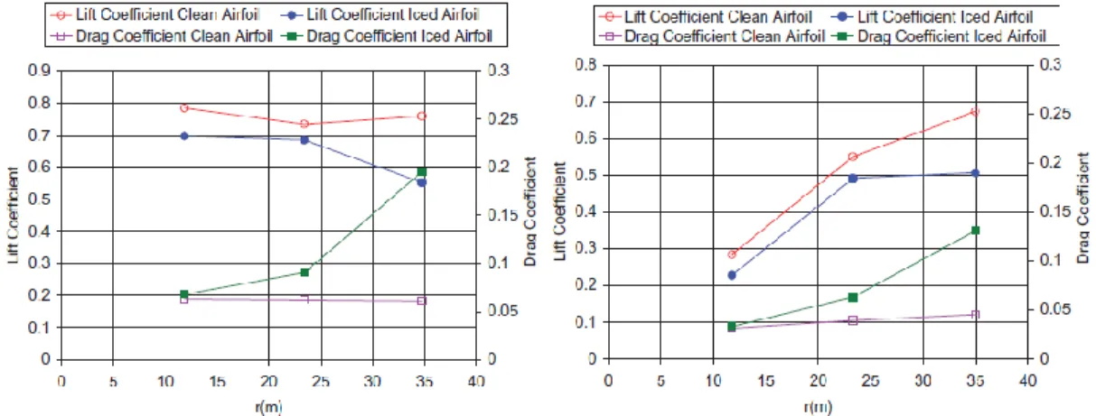
In a study by Hochart et al. (2008), different scaled sections of the 1.8 MW Vestas V80 wind turbine were tested in a stationary, multiphase flow wind tunnel. The wind tunnel tests took place at the Anti-Icing Materials International Laboratory (AMIL) at the University of Quebec in Chicoutimi (UQAC). The NACA 63415 airfoil was used for the airfoil of the blade, as the nature of the original airfoil was unknown. Three different radial positions of the V80 rotor were tested at 12, 23.5 and 35 m of a 40 m blade. The relative velocity and angle of attack of each section were calculated for application in the wind tunnel. The icing conditions measured in Murdochville, where the Vestas V80 turbine is located, were applied in the refrigerated wind
tunnel. Two different in-cloud icing conditions were simulated, as follows: -1.4oC with an LWC of 0.218 g/m3 and a wind speed of 8.8 m/s for 6 hours; and -5.7oC with an LWC of 0.242 g/m3 and a wind speed of 4.2 m/s for 4.4 hours.
As seen in Figure 1-2, during the first icing event with glaze ice formation (at -1.4oC), drag increases and lift decreases due to icing. This change seems more dramatic towards the tip of the blade, where the amount of ice increases due to higher rotational speed. During the second icing event (at -5.7oC), where rime ice occurs, a less dramatic increase in drag and a reduction in lift are observed, as the weight of the rime ice is less than that of the glaze ice. The decrease in lift is found to be around 40% at the tip of the blade for both types of icing. The drag increases by about 365% and 250% at the tip during glaze and rime icing events respectively.
Figure 1-2 Lift and drag coefficient change with glaze and rime icing respectively. Hochart et al. (2008)
1.3 Numerical Investigation of Icing
1.3.1 Collection Efficiency Analysis
A crucial parameter for simulating icing is collection efficiency, which is the rate of accumulation of supercooled droplets on the surface. It is called catch efficiency or collision
efficiency in many studies. A significant number of studies have been carried out on this subject,
as the weight of the ice accumulating on a surface is directly related to this parameter. Multiphase analysis of the ice, which is composed of air and water droplets, is needed in order to compute collection efficiency. In the literature, two type of multiphase analysis are performed:
Lagrangian and Eulerian. In Lagrangian analysis, the trajectory of the each water particle present in the airflow is calculated, whereas in Eulerian analysis, the water phase is considered as a continuum, like the air phase.
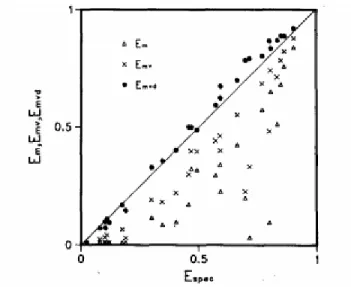
As the size of the water droplets varies within a range, either all the droplet sizes must be represented, or they must be approximated in a single-sized droplet. Since the second alternative is more practical and more cost-effective, it is the preferred option in many studies. A comparative study by Finstad et al. (1988) showed that the Median Volume Diameter (MVD) approach represents the flow better than the other approaches, namely, Mean Volume Diameter and Mean Diameter. Figure 1-3 shows the collision efficiency for single-size approximation methods and spectral weighted analysis. As we can see, the MVD approach and spectral weighted analysis, in which all the droplet sizes are represented, are well matched.
Figure 1-3 Comparison of collision efficiencies for single-size approximation methods and spectral weighted analysis. (Finstad, Lozowski and Makkonen 1988)
The study of Silveria et al. (2003) presents the collection efficiency calculated on various bodies with Lagrangian and Eulerian methods. The authors made a few assumptions for both methods: initially, the water droplets are rigid spheres, which means that the constant drag factor can be used without considering variations in the shape of the droplets; the droplets do not affect airflow, since the water concentration is negligible; finally, gravity is ignored, since the droplets are small. For the Eulerian case, full multiphase simulation was performed using the commercial tool CFX 5.5. In this model, the governing equations for mass, momentum and energy are solved
for both air and water. A phase volume fraction equation is also solved. For the turbulence treatment, the model is applied to the main phase, and the zero-equation model is applied to the dispersed phase for improved convergence and numerical stability.
A comparison of multiphase analysis with experimental data for the NACA 0012 airfoil is shown in Figure 1-4.
Figure 1-4 Collection efficiency comparison for the NACA 0012 (Silveria, et al. 2003) The Lagrangian approach gives better results for 2D cases (Silveria et al. 2008). However, for 3D and complex geometries, the use of the Eulerian approach is more appropriate, as it is difficult to make a prediction for the location to inject particles that would hit to wall domains for the Lagrangian method. Moreover, trajectory calculation for each droplet is not cost-effective for a 3D domain.
1.3.2 Ice Shape Computation
Once the accretion rate has been calculated, the ice shape can be determined from a thermodynamic analysis. The Messinger model (Myers 2001), which appears in many icing codes, such as LEWICE and DRA, consists of an energy balance based on equating the heat lost to the air from ice and water accretion and the production of latent heat due to ice growth. The heat loss mechanism includes convective heat transfer at the water surface, evaporative heat loss
and cooling by incoming droplets. In contrast, the gain mechanism includes the kinetic energy of incoming droplets, the release of latent heat and aerodynamic heating.
However, while Messinger’s model is the solution for 1D energy balance equations for an insulated and unheated surface exposed to icing, it has some limitations. The transitional behavior cannot be captured, since the temperature is set in an equilibrium state. Moreover, no conduction between the ice and water layers and the surface of the substrate is modeled. This assumption may cause the model to predict less ice accretion on that surface.
A more developed version of Messinger’s model has been proposed by Myers (2001), which is known as the Extended Messinger method. The system consists of four equations: heat transfer equations for ice and water, a mass balance equation and a phase change equation, known as the Stefan equation. For this model, ice is assumed to have a perfect thermal contact with the surface, so that the ice temperature at the surface is equal to the surface temperature. Moreover, temperature is continuous at the phase change boundary, and is equal to the freezing temperature. Rime ice thickness is calculated by setting the water thickness to zero, so that only the mass balance equation is solved to calculate ice thickness and temperature. In contrast, the glaze ice is a fraction of the water mass flux on the surface transformed into ice. Another fraction remains as a water layer.
An overview of the ice shape prediction codes and some applications are given below. LEWICE 3.0
LEWICE (Wright 2005), developed by NASA’s Glenn Research Center, is an ice growth prediction code for aircraft. It is updated periodically, in response to advances made in the theoretical background of icing physics. LEWICE is made up of four main modules for the computation of flow field: particle trajectory, mass and energy balance equations, and updated ice shape. The mass and energy balance equations are based on the Messinger model, which accounts for the convection, latent heat transfer, aerodynamic heating and enthalpy change of the water. Heat transfer coefficients are calculated via the Integral Boundary Layer method. For the ice shape calculation, a multilayer approach is used, which enables computation of the step-by-step growth of ice throughout total ice exposure interval.
The latest version of the model, LEWICE 3.0 [24], is capable of 3D icing simulation using either the Navier-Stokes equations or potential flow equations with various droplet mechanisms, like splashing and SLDs.
TURBICE
Makkonen et al. (2001) presented an icing code, TURBICE, to simulate glaze and rime icing on wind turbines. TURBICE uses a panel method for flow field prediction, in which the number of panels is optimized considering the accuracy of the computed local collision efficiency distribution. Potential flow and droplet trajectory analysis are repeated for each layer. Local collision efficiency is a ratio of the space between the droplets away from blade to the space between the droplets near the blade. For multiple size droplets, the Median Volume Diameter approach, which is the best single size parameter approximation method, was used. Ice density is calculated using an empirical correlation called the Macklin parameter, which depends on MVD, free stream wind speed and surface temperature. The heat transfer model is based on mass and energy balance equations. The freezing fraction and surface temperature are calculated by solving these equations at each finite element section on the blade surface. When the freezing fraction is between 0 and 1, the wet growth, runback water is taken into account.
Ice accretion on a NACA 64618, representing a 5 MW pitch controlled blade, has been simulated numerically to investigate the effect of temperature and droplet size on ice accretion by Homola et al. (2010). The commercial CFD code, ANSYS FLUENT, is used to simulate the iced blade, owing to its ability to model complex flows. A structured grid is used with a boundary layer resolution that ensures that y+ is less than 10. The k- turbulence model is used with a log-law function to resolve the thin boundary layer. The authors numerically tested various icing conditions at -2.5oC, -5oC and -7.5oC, and with an MVD of 12, 17 and 30 m. Results are shown for 17 m for the investigation of effect of temperature on icing. At -2.5o
C, the ice shape shows a horn-like structure, whereas at -5oC and -7.5oC, the ice shape follows the contours of the airfoil, as shown in Figure 1-5. This is because the first shape consists of glaze icing and the others consist of rime icing, as explained above.
Figure 1-5 Effect of temperature on ice shape calculation (Homola, et al. 2010)
CFD analysis of these profiles shows that, compared to a clean blade, the flow over all the iced blades separates at lower angles of attack. However, the separation is the most dramatic for the glaze iced blade, owing to its horn-like shape. Also, comparison of the aerodynamic coefficients shows that the lift coefficient decreases and the drag coefficient increases as the horn characteristics become more pronounced. The effect of droplet size was tested at -2.5oC. The resulting ice shapes are shown in Figure 1-6. As we can see, the icing area grows with increasing droplet size. This is because the larger droplets have more inertia and are less affected by air drag. The horn structure, which is a characteristic of glaze icing, is not observed for the smallest droplet size of MVD 12 m. The results of the CFD analysis on iced blades show that, as the MDV increases, the size of the recirculation and separation zone also increases. Moreover, the lift coefficient decreases and the drag coefficient increases with increasing droplet size.
FENSAP-ICE-Unsteady
A methodology for the simulation of icing on various machines is presented by Aliaga et al. (2010). FENSAP-ICE-Unsteady has the ability to predict ice shape on Aircraft, Rotorcraft and jet engines using the 3D Unsteady Navier-Stokes equations for flow field analysis (FENSAP module) and the Eulerian method for water droplet trajectory analysis (DROP 3D module). Although FENSAP-ICE-Unsteady is very profitable in terms of computing unsteady impingement on a surface, it is not cost-effective, since 2,100 rotor rotations are needed for 1 minute of icing simulation of a helicopter blade.
OTHER CODES
Although there are a variety of codes in the literature, the methodology on which they are based is similar. The most popular codes are Bombardier’s CANICE, Italy’s CIRAMIL, France’s ONERA, and the UK’s ICECREMO and DRA.
1.4 Iced Airfoil & Blade Aerodynamics
Lee et al. (2000) presented a review on the effects of several parameters on iced airfoil aerodynamic characteristics, such as the lift, drag and pitching moment coefficients. Results are derived from a series of wind tunnel analyses investigating the effects of the ice shape, its size and location on the airfoil, the flight Reynolds number and the airfoil geometry.
As stated above, as the ice thickness increases, the performance of the airfoil decreases as a consequence of the reduction in lift and the increase in drag. However, the leading edge of the airfoil is an exception, as its performance does not deteriorate beyond a critical ice height. Moreover, experiments on ice shape show that, as the ice shape becomes blunter, that is, free of sharp edges, the maximum lift coefficient decreases less. The presence of roughness elements of different heights and of glaze ice have also been studied and it has been shown that the performance of an iced airfoil becomes insensitive to increases in Reynolds number beyond a certain value of that number.
A study by Bragg et al. (2005) classifies ice formations according to their shape and evaluates their influence on airfoil aerodynamics. The roughness type of the ice formation is defined in that work at the initial stages of icing, where the icing particles create small perturbations on the airfoil surface. Streamwise ice follows the contour of the airfoil, which is typical for rime icing. Horn-type ice has a horn shape at the leading edge, as its name implies. Finally, ridge-type ice refers to the relatively large pieces of ice that are located separately on the airfoil. The latter type of icing is associated with SLDs. Experiments show that the roughness type of ice formation causes early transition of the flow at low Reynolds numbers. As the Reynolds number increases further, the transition area over the airfoil grows relative to that of a clean airfoil. Moreover, the increase in the area covered by the roughness ice results in a larger transition area on the airfoil. For horn-type ice, separation is observed just downstream of the horn. As the angle of attack increases, the separation area increases further, as seen in Figure 1-7. An increase in the bubble area causes the drag coefficient to grow, which ultimately results in a stall at a critical angle of attack.
Figure 1-7 Flow separation over horn ice for the NACA 0012. (Bragg, Broeren and Blumenthal 2005)
Comparison of horn-iced airfoils with a clean airfoil show that iced airfoils stall at smaller angles of attack, as seen in Figure 1-8. Moreover, iced airfoils with a different horn tip radius show almost the same lift coefficient curves, which means that the horn tip radius has no effect on the lift coefficient.