A modified ICP algorithm for normal-guided surface registration
Texte intégral
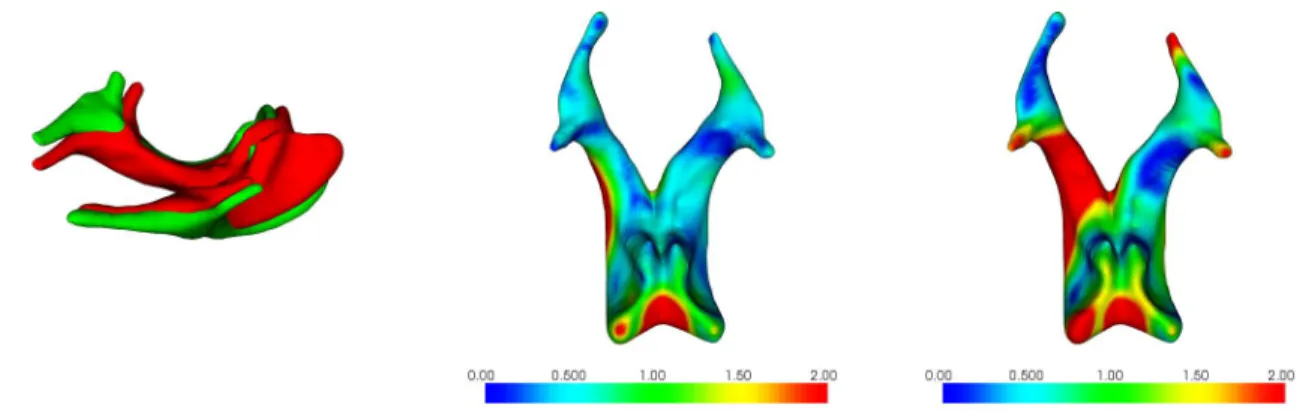
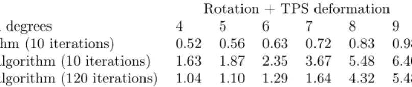
Figure
Documents relatifs
Here are the key characteristic prop- erties of this pseudovariety, which combine the results of [8], dealing with pseudovarieties of ordered monoids, with the observations of
Nos compétences pédagogiques et techniques variées (coordination, expertise bibliographique, enseignement-formation, communication/conception de supports, maîtrise de
The purpose of the performance evaluation was threefold: (1) analyzing the effect of algorithm parameters and forest structure and com- position on the registration errors,
In order to test the performance of the different algorithms in terms of estimating transformation parameters for the registration of surfaces affected by noise, noise
the previously selected pairs, the points (p3-m2) corresponding to the minimum distance (d2) of the resulting matrix are then chosen as another match, and so on. As illustrated
Without using the rows and columns of the previously selected pairs, the points (p3-m2) corresponding to the minimum distance (d2) of the resulting matrix are then chosen as
The jet energy scale, jet energy resolution, and their systematic uncertainties are measured for jets reconstructed with the ATLAS detector in 2012 using proton–proton data produced
Both the steady-state size and growth rate of accretions on a test article with a hemispherical nose were duplicated in tests conducted at pressures of 34.5 kPa (5 psia) and 69 kPa
