Option Valuation with Long-run and Short-run Volatility Components

Texte intégral

(1)2004s-56. Option Valuation with Longrun and Short-run Volatility Components Peter Christoffersen, Kris Jacobs, Yintian Wang. Série Scientifique Scientific Series. Montréal Novembre 2004. © 2004 Peter Christoffersen, Kris Jacobs, Yintian Wang. Tous droits réservés. All rights reserved. Reproduction partielle permise avec citation du document source, incluant la notice ©. Short sections may be quoted without explicit permission, if full credit, including © notice, is given to the source..

(2) CIRANO Le CIRANO est un organisme sans but lucratif constitué en vertu de la Loi des compagnies du Québec. Le financement de son infrastructure et de ses activités de recherche provient des cotisations de ses organisations-membres, d’une subvention d’infrastructure du Ministère du Développement économique et régional et de la Recherche, de même que des subventions et mandats obtenus par ses équipes de recherche. CIRANO is a private non-profit organization incorporated under the Québec Companies Act. Its infrastructure and research activities are funded through fees paid by member organizations, an infrastructure grant from the Ministère du Développement économique et régional et de la Recherche, and grants and research mandates obtained by its research teams. Les organisations-partenaires / The Partner Organizations PARTENAIRE MAJEUR . Ministère du Développement économique et régional et de la Recherche [MDERR] PARTENAIRES . Alcan inc. . Axa Canada . Banque du Canada . Banque Laurentienne du Canada . Banque Nationale du Canada . Banque Royale du Canada . Bell Canada . BMO Groupe Financier . Bombardier . Bourse de Montréal . Caisse de dépôt et placement du Québec . Développement des ressources humaines Canada [DRHC] . Fédération des caisses Desjardins du Québec . GazMétro . Hydro-Québec . Industrie Canada . Ministère des Finances du Québec . Norshield Asset Management (Canada) Ltd. . Pratt & Whitney Canada Inc. . Raymond Chabot Grant Thornton . Ville de Montréal . École Polytechnique de Montréal . HEC Montréal . Université Concordia . Université de Montréal . Université du Québec à Montréal . Université Laval . Université McGill . Université de Sherbrooke ASSOCIE A : . Institut de Finance Mathématique de Montréal (IFM2) . Laboratoires universitaires Bell Canada . Réseau de calcul et de modélisation mathématique [RCM2] . Réseau de centres d’excellence MITACS (Les mathématiques des technologies de l’information et des systèmes complexes) Les cahiers de la série scientifique (CS) visent à rendre accessibles des résultats de recherche effectuée au CIRANO afin de susciter échanges et commentaires. Ces cahiers sont écrits dans le style des publications scientifiques. Les idées et les opinions émises sont sous l’unique responsabilité des auteurs et ne représentent pas nécessairement les positions du CIRANO ou de ses partenaires. This paper presents research carried out at CIRANO and aims at encouraging discussion and comment. The observations and viewpoints expressed are the sole responsibility of the authors. They do not necessarily represent positions of CIRANO or its partners.. ISSN 1198-8177.

(3) Option Valuation with Long-run and Short-run Volatility Components* Peter Christoffersen†, Kris Jacobs‡, Yintian Wang§ Résumé / Abstract Ce papier présente un nouveau modèle d’évaluation d’options européennes. Dans notre modèle, la volatilité des rendements se décompose en deux parties. Une des composantes est une composante de long terme, et elle peut être modélisée comme permanente. L’autre composante porte sur le court terme et est de moyenne nulle. Notre modèle peut être considéré comme la version affine de Engle & Lee (1999), permettant l’évaluation simple d’options européennes. Nous étudions le modèle à travers une analyse intégrée de données de rendements et d’options. La performance du modèle est spectaculaire comparée à un benchmark tel qu’un modèle à une seule composante de volatilité bien connu dans la littérature. L’amélioration de la performance du modèle est due à une dynamique plus riche qui permet de modéliser conjointement des options à maturité longue et à maturité courte. Mots clés : évaluation d’option, composante long terme, composante court terme, composantes non observables, persistance, GARCH, hors échantillon. This paper presents a new model for the valuation of European options. In our model, the volatility of returns consists of two components. One of these components is a long-run component, and it can be modeled as fully persistent. The other component is short-run and has a zero mean. Our model can be viewed as an affine version of Engle and Lee (1999), allowing for easy valuation of European options. We investigate the model through an integrated analysis of returns and options data. The performance of the model is spectacular when compared to a benchmark single-component volatility model that is well-established in the literature. The improvement in the model’s performance is due to its richer dynamics which enable it to jointly model long-maturity and short-maturity options. Keywords: option valuation, long-run component, short-run component, unobserved components, persistence, GARCH, out-of-sample. Codes JEL : G12. * The first two authors are grateful for financial support from FQRSC, IFM2 and SSHRC. We would like to thank Tim Bollerslev, Frank Diebold, Bjorn Eraker, Steve Heston, Robert Hauswald, Eric Jacquier, Nour Meddahi, Michel Robe, Jean-Guy Simonato and seminar participants at American University, HEC Montreal and McGill University for helpful remarks and discussions. Any remaining inadequacies are ours alone. † McGill University and CIRANO. ‡ Address for correspondence: CIRANO and Department of Finance, Faculty of Management, McGill University, 1001 Sherbrooke Street West, Montreal, QC, Canada, H3A 1G5, tel: 514-398-4025, email: [email protected]. § McGill University..

(4) 1. Introduction. There is a consensus in the literature that combining time-variation in the conditional variance of asset returns (Engle (1982), Bollerslev (1986)) with a leverage effect (Black (1976)) constitutes a potential solution to well-known biases associated with the Black-Scholes (1973) model, such as the smile and the smirk. To model the smirk, these models generate higher prices for out-of-the-money put options as compared to the Black-Scholes formula. Equivalently, the models generate negative skewness in the distribution of asset returns. In the continuous-time option valuation literature, the Heston (1993) model addresses some of these biases. This model contains a leverage effect as well as stochastic volatility.1 In the discretetime literature, the NGARCH(1,1) option valuation model proposed by Duan (1995) contains time-variation in conditional variance as well as a leverage effect. The model by Heston and Nandi (2000) is closely related to Duan’s model. Many existing empirical studies have conÞrmed the importance of time-varying volatility and the leverage effect in continuous-time and discrete-time setups.2 However, it has become clear that while these models help explain the biases of the Black-Scholes model in a qualitative sense, they come up short in a quantitative sense. Using parameters estimated from returns or options data, these models reduce the biases of the Black-Scholes model, but the magnitude of the effects is insufficient to completely resolve the biases. The resulting pricing errors have the same sign as the Black-Scholes pricing errors, but are smaller in magnitude. We therefore need models that possess the same qualitative features as the models in Heston (1993) and Duan (1995), but that contain stronger quantitative effects. These models need to generate more ßexible skewness and volatility of volatility dynamics in order to Þt observed option prices. One interesting approach in this respect is the inclusion of jump processes. In most existing studies, jumps are added to models that already contain time-variation in the conditional variance as well as a leverage effect. The empirical Þndings in this literature have been mixed. In general jumps in returns and volatility improve option valuation when parameters are estimated using historical time series of returns, but usually not when parameters are estimated using the cross-section of option prices.3 This paper takes a different approach. We attempt to remedy the remaining option biases by modeling richer volatility dynamics.4 It has been observed using a variety of 1. The importance of stochastic volatility is also studied in Hull and White (1987), Melino and Turnbull (1990), Scott (1987) and Wiggins (1987). 2 See for example Amin and Ng (1993), Bakshi, Cao and Chen (1997), Bates (1996, 2000), Benzoni (1998), Bollerslev and Mikkelsen (1999), Chernov and Ghysels (2000), Duan, Ritchken and Sun (2004), Engle and Mustafa (1992), Eraker (2004), Heston and Nandi (2000), Jones (2003), Nandi (1998) and Pan (2003). 3 See for example Bakshi, Cao and Chen (1997), Eraker, Johannes and Polson (2003), Eraker (2004) and Pan (2002). 4 Adding jumps to the new volatility speciÞcation may of course improve the model further.. 2.

(5) diagnostics that it is difficult to Þt the autocorrelation function of return volatility using a benchmark model such as a GARCH(1,1). Even though the comparison between discrete and continuous-time models is sometimes tenuous (see Corradi (2000)), similar remarks apply to stochastic volatility models such as Heston (1993). The main problem is that volatility autocorrelations are too high at longer lags to be explained by a GARCH(1,1), unless the process is extremely persistent. This extreme persistence may impact negatively on other aspects of option valuation, such as the valuation of short-maturity options. In fact, it has been observed in the literature that volatility may be better modeled using a fractionally integrated process, rather than a stationary GARCH process.5 Andersen, Bollerslev, Diebold and Labys (2003) conÞrm this Þnding using realized volatility. Bollerslev and Mikkelsen (1996, 1999) and Comte, Coutin and Renault and (2001) investigate and discuss some of the implications of long memory for option valuation. Using fractional integration models for option valuation is cumbersome. Optimization is very time-intensive and a number of ad-hoc choices have to be made regarding implementation. This paper addresses the same issues using a different type of model that is easier to implement and captures the stylized facts addressed by long-memory models at horizons relevant for option valuation. The model builds on Heston and Nandi (2000) and Engle and Lee (1999). In our model, the volatility of returns consists of two components. One of these components is a long-run component, and it can be modeled as (fully) persistent. The other component is short-run and mean zero. The model is able to generate autocorrelation functions that are richer than those of a GARCH(1,1) model while using just a few additional parameters. We illustrate how this impacts on option valuation by studying the term structure of volatility. Unobserved component or factor models are very popular in the Þnance literature. See Fama and French (1988), Poterba and Summers (1988) and Summers (1986) for applications to stock prices. In the option pricing literature, Bates (2000) and Taylor and Xu (1994) investigate two-factor stochastic volatility models. Eraker (2004) suggests the usefulness of our approach based on stylized facts emanating from his empirical study. Alizadeh, Brandt and Diebold (2002) uncover two factors in stochastic volatility models of exchange rates using range-based estimation. Unobserved component models are also very popular in the term structure literature, although in this literature the models are more commonly referred to as multifactor models.6 There are very interesting parallels between our approach and results and stylized facts in the term structure literature. In the term structure literature it is customary to model short-run ßuctuations around a time-varying long-run mean of the short rate. In our framework we model short-run ßuctuations around time-varying long-run volatility. Dynamic factor and component models can be implemented in continuous or discrete 5. See Baillie, Bollerslev and Mikkelsen (1996) and Chernov, Gallant, Ghysels and Tauchen (2003). See for example Dai and Singleton (2000), Duffee (1999), Duffie and Singleton (1999) and Pearson and Sun (1994). 6. 3.

(6) time. We choose a discrete-time approach because of the ease of implementation. In particular, our model is related to the GARCH class of processes and volatility Þltering and forecasting are relatively straightforward, which is critically important for option valuation. An additional advantage of our model is parsimony: the most general model we investigate has seven parameters. The models with jumps in returns and volatility discussed above are much more heavily parameterized. We speculate that parsimony may help our model’s out-of-sample performance. We investigate the model through an integrated analysis of returns and options data. We study two models: one where the long-run component is constrained to be fully persistent and one where it is not. We refer to these models as the persistent component model and the component model respectively. When persistence of the long-run component is freely estimated, it is very close to one. The performance of the component model is spectacular when compared with a benchmark GARCH(1,1) model. The improvement in the model’s performance is due to its richer dynamics, which enable it to jointly model long-maturity and short-maturity options. Our out-of-sample results strongly suggest that these richer dynamics are not simply due to spurious in-sample overÞtting. The persistent component model performs better than the benchmark GARCH(1,1) model, but it is inferior to the component model both in- and out-of-sample. We also provide a detailed study of the term structure of volatilities for our proposed models and the benchmark model. The paper proceeds as follows. Section 2 introduces the model. Section 3 discusses the volatility term structure and Section 4 discusses option valuation. Section 5 discusses the empirical results, and Section 6 concludes.. 2. Return Dynamics with Volatility Components. In this section we Þrst present the Heston-Nandi GARCH(1,1) model which will serve as the benchmark model throughout the paper. We then construct the component model as a natural extension of a rearranged version of the GARCH(1,1) model. Finally the persistent component model is presented as a special case of the component model.. 2.1. The Heston and Nandi GARCH(1,1) Model. Heston and Nandi (2000) propose a class of GARCH models that allow for a closed-form solution for the price of a European call option. They present an empirical analysis of the GARCH(1,1) version of this model, which is given by p ln(St+1 ) = ln(St ) + r + λht+1 + ht+1 zt+1 (1) p ht+1 = w + b1 ht + a1 (zt − c1 ht )2 4.

(7) where St+1 denotes the underlying asset price, r the risk free rate, λ the price of risk and ht+1 the daily variance on day t + 1 which is known at the end of day t. The zt+1 shock is assumed to be i.i.d. N (0, 1). The Heston-Nandi model captures time variation in the conditional variance as in Engle (1982) and Bollerslev (1986),7 and the parameter c1 captures the leverage effect. The leverage effect captures the negative relationship between shocks to returns and volatility (Black (1976)), which results in a negatively skewed distribution of returns. Its importance for option valuation has been emphasized among others by Benzoni (1998), Chernov and Ghysels (2000), Christoffersen and Jacobs (2004), Eraker (2004), Eraker, Johannes and Polson (2003), Heston (1993), Heston and Nandi (2000) and Nandi (1998). It must be noted at this point that the GARCH(1,1) dynamic in (1) is slightly different from the more conventional NGARCH model used by Engle and Ng (1993) and Hentschel (1995), which is used for option valuation in Duan (1995). The reason is that the dynamic in (1) is engineered to yield a closed-form solution for option valuation, whereas a closed-form solution does not obtain for the more conventional GARCH dynamic. Hsieh and Ritchken (2000) provide evidence that the more traditional GARCH model may actually slightly dominate the Þt of (1). Our main point can be demonstrated using either dynamic. Because of the convenience of the closed-form solution provided by dynamics such as (1), we use this as a benchmark in our empirical analysis and we model the richer component structure within the Heston-Nandi framework. To better appreciate the workings of the component models presented below, note that by using the expression for the unconditional variance E [ht+1 ] ≡ σ 2 =. w + a1 1 − b1 − a1 c21. the variance process can now be rewritten as ´ ³ p ¡ ¢ ht+1 = σ 2 + b1 ht − σ 2 + a1 (zt − c1 ht )2 − (1 + c21 σ 2 ). 2.2. (2). Building a Component Volatility Model. The expression for the GARCH(1,1) variance process in (2) highlights the role of the parameter σ 2 as the constant unconditional mean of the conditional variance process. A natural generalization is then to specify σ 2 as time-varying. Denoting this time-varying component by qt+1 , the expression for the variance in (2) can be generalized to ³ ´ p (3) ht+1 = qt+1 + β (ht − qt ) + α (zt − γ 1 ht )2 − (1 + γ 21 qt ). This model is similar in spirit to the component model of Engle and Lee (1999). The difference between our model and Engle and Lee (1999) is that the functional form of the 7. For an early application of GARCH to stock returns, see French, Schwert and Stambaugh (1987).. 5.

(8) GARCH dynamic (3) allows for a closed-form solution for European option prices. This is similar to the difference between the Heston-Nandi (2000) GARCH(1,1) dynamic and the more traditional NGARCH(1,1) dynamic discussed in the previous subsection. In speciÞcation (3), the conditional volatility ht+1 can most usefully be thought of as consisting of two components. Following Engle and Lee (1999), we refer to the component qt+1 as the long-run component, and to ht+1 − qt+1 as the short-run component. We will discuss this terminology in some more detail below. Note that by construction the unconditional mean of the short-run component ht+1 − qt+1 is zero. The model can also be written as ³ ´ p ht+1 = qt+1 + (αγ 21 + β) (ht − qt ) + α (zt − γ 1 ht )2 − (1 + γ 21 ht ) ³ ´ p 2 2 ˜ = qt+1 + β (ht − qt ) + α (zt − γ 1 ht ) − (1 + γ 1 ht ) (4) where β˜ = αγ 21 + β. This representation is useful because we can think of ³ p ´2 zt − γ 1 ht − (1 + γ 21 ht ) p ¢ ¡ = zt2 − 1 − 2γ 1 ht zt. v1,t ≡. (5). as a mean-zero innovation. The model is completed by specifying the functional form of the long-run volatility component. In a Þrst step, we assume that qt+1 follows the process ´ ³¡ p ¢ 2 (6) qt+1 = ω + ρqt + ϕ zt − 1 − 2γ 2 ht zt. Note that we can therefore write the component volatility model as ˜ (ht − qt ) + αv1,t ht+1 = qt+1 + β qt+1 = ω + ρqt + ϕv2,t with. p ¡ ¢ vi,t = zt2 − 1 − 2γ i ht zt , for i = 1, 2.. (7). (8). ˜ γ1, and Et−1 [vi,t ] = 0, i = 1, 2. Also note that the model contains seven parameters: α, β, γ 2 , ω, ρ and ϕ in addition to the price of risk, λ.. 2.3. A Fully Persistent Special Case. In our empirical work, we also investigate a special case of the model in (7). Notice that in (7) the long-run component of volatility will be a mean reverting process for ρ < 1. We also 6.

(9) estimate a version of the model which imposes ρ = 1. The resulting process is ˜ (ht − qt ) + αv1,t ht+1 = qt+1 + β qt+1 = ω + qt + ϕv2,t. (9). ˜ γ 1 , γ 2 , ω and ϕ in and vi,t , i = 1, 2 as in (8). The model now contains six parameters: α, β, addition to the price of risk, λ. In this case the process for long-run volatility contains a unit root and shocks to the longrun volatility never die out: they have a “permanent” effect. Recall that following Engle and Lee (1999) in (7) we refer to qt+1 as the long-run component and to ht+1 − qt+1 as the short-run component. In the special case (9) we can also refer to qt+1 as the “permanent” component, because innovations to qt+1 are truly “permanent” and do not die out. It is then customary to refer to ht+1 − qt+1 as the “transitory” component, which reverts to zero. It is in fact this permanent-effects version of the model that is most closely related to models which have been studied more extensively in the Þnance and economics literature, rather than the more general model in (7).8 We will refer to this model as the persistent component model. It is clear that (9) is nested by (7). It is therefore to be expected that the in-sample Þt of (7) is superior. However, out-of-sample this may not necessarily be the case. It is often the case that more parsimonious models perform better out-of-sample if the restriction imposed by the model is a sufficiently adequate representation of reality. The persistent component model may also be better able to capture structural breaks in volatility out-ofsample, because a unit root in the process allows it to adjust to a structural break, which not possible for a mean-reverting process. It will therefore be of interest to verify how close ρ is to one when estimating the more general model (7).. 3. Variance Term Structures. To intuitively understand the shortcomings of existing models such as the GARCH(1,1) model in (1) and the improvements provided by our model (7), it is instructive to graphically illustrate the workings of both models in a dimension that critically affects their performance. In this section we graphically illustrate the variance term structures and some other related properties of the models that are key for option valuation. 8. See Fama and French (1988), Poterba and Summers (1988) and Summers (1986) for applications to stock prices. See Beveridge and Nelson (1981) for an application to macroeconomics.. 7.

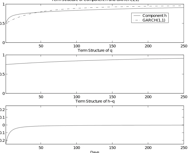
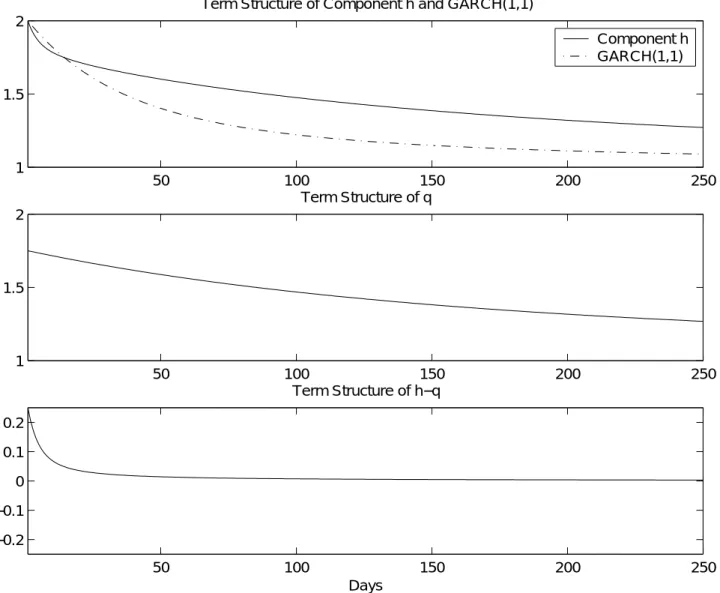
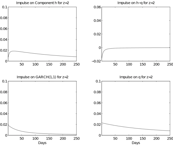
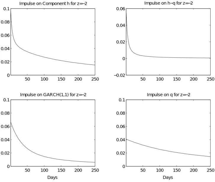
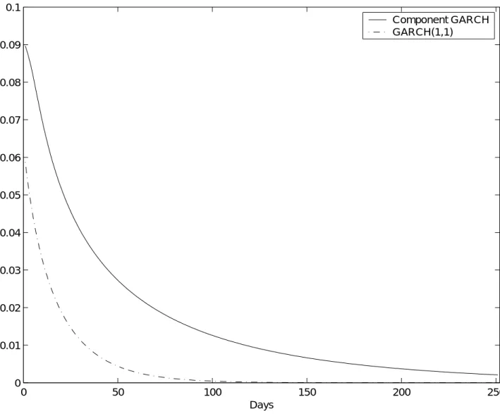
(10) 3.1. The Variance Term Structure for the GARCH(1,1) Model. Following the logic used for the component model in (7), we can rewrite the GARCH(1,1) variance dynamic in (2). We have ³ ´ p ¡ ¢ ht+1 = σ 2 + ˜b1 ht − σ 2 + a1 (zt2 − 1) − 2c1 ht zt (10). where ˜b1 = b1 + a1 c21 and where the innovation term has a zero conditional mean. From (10) the multi-step forecast of the conditional variance is 2 Et [ht+k ] = σ 2 + ˜bk−1 1 (ht+1 − σ ). where the conditional expectation is taken at the end of day t. Notice that ˜b1 is directly interpretable as the variance persistence in this representation of the model. We can now deÞne a convenient measure of the variance term structure for maturity K as ht+1:t+K. K K 2 1 X 1 X 2 ˜k−1 1 − ˜bK 1 (ht+1 − σ ) ≡ Et [ht+k ] = σ + b1 (ht+1 − σ 2 ) = σ 2 + K k=1 K k=1 K 1 − ˜b1. This variance term structure measure succinctly captures important information about the model’s potential for explaining the variation of option values across maturities.9 To compare different models, it is convenient to set the current variance, ht+1 , to a simple m multiple of the long run variance. In this case the variance term structure relative to the unconditional variance is given by 1 − ˜bK 1 (m − 1) ht+1:t+K /σ 2 ≡ 1 + K 1 − ˜b1 The bottom-left panels of Figures 1 and 2 show the term structure of variance for the GARCH(1,1) model for a low and high initial conditional variance respectively. We use parameter values estimated via MLE on daily S&P500 returns (the estimation details are in Table 2 and will be discussed further below). We set m = 12 in Figure 1 and m = 2 in Figure 2. The Þgures present the variance term structure for up to 250 days, which corresponds approximately to the number of trading days in a year and therefore captures the empirically relevant term structure for option valuation. It can be clearly seen from Figures 1 and 2 that for the GARCH(1,1) model, the conditional variance converges to the long-run variance rather fast. We can also learn about the dynamics of the variance term structure though impulse response functions. For the GARCH(1,1) model, the effect of a shock at time t, zt , on the 9. Notice that due to the price of risk term in the conditional mean of returns, the term structure of variance as deÞned here is not exactly equal to the conditional variance of cumulative returns over K days.. 8.

(11) expected k-day ahead variance is ³ ´ p a h /z 1 − c ∂(Et [ht+k ])/∂zt2 = ˜bk−1 1 1 t t 1. and thus the effect on the variance term structure is ∂Et [ht:t+K ] /∂zt2 =. ³ ´ p 1 − ˜bK 1 a1 1 − c1 ht /zt 1 − ˜b1 K. The bottom-left panels of Figures 3 and 4 plot the impulse responses to the term structure of variance for ht = σ 2 and zt = 2 and zt = −2 respectively, again using the parameter estimates from Table 2. The impulse responses are normalized by the unconditional variance. Notice that the effect of a shock dies out rather quickly for the GARCH(1,1) model. Comparing across Figures 3 and 4 we see the asymmetric response of the variance term structure from a positive versus negative shock to returns. This can be thought of as the term structure of the leverage effect. Due to the presence of a positive c1 , a positive shock has less impact than a negative shock along the entire term structure of variance.. 3.2. The Variance Term Structure for the Component Model. In the component model we have ˜ (ht − qt ) + αv1,t ht+1 = qt+1 + β qt+1 = ω + ρqt + ϕv2,t The multi-day forecast of the two components are k−1 Et [ht+k − qt+k ] = β˜ (ht+1 − qt+1 ) ³ ´ ω ω + ρk−1 qt+1 − 1−ρ Et [qt+k ] = 1−ρ ¡ ¢ ≡ σ 2 + ρk−1 qt+1 − σ 2. The simplicity of these multi-day forecasts is a key advantage of the component model. The multi-day variance forecast is a simple sum of two exponential components. Notice that β˜ and ρ correspond directly to the persistence of the short-run and long-run components respectively. We can now calculate the variance term structure in the component model for maturity. 9.

(12) K as ht+1:t+K ≡. K 1 X Et [qt+k ] + Et [ht+k − qt+k ] K k=1. K ¡ ¢ 1 X 2 k−1 = σ + ρk−1 qt+1 − σ 2 + β˜ (ht+1 − qt+1 ) K k=1 K 1 − ρK qt+1 − σ 2 1 − β˜ ht+1 − qt+1 = σ + + 1−ρ K K 1 − β˜ 2. If we set qt+1 and ht+1 equal to m1 and m2 multiples of the long run variance respectively, then we get the variance term structure relative to the unconditional variance simply as K 1 − ρK m1 − 1 1 − β˜ m2 − m1 ht+1:t+K /σ = 1 + + 1−ρ K K 1 − β˜ 2. (11). The top-left panels in Figures 1 and 2 show the term structure of variance for the component model using parameters estimated via MLE on daily S&P500 returns from Table 2. We set m1 = 34 , m2 = 12 in Figure 1 and m1 = 74 , m2 = 2 in Figure 2. By picking m2 equal to the m used for the GARCH(1,1) model, we ensure comparability across models within each Þgure because the spot variances relative to their long-run variances are identical.10 The main conclusion from Figures 1 and 2 is that compared to the bottom-left panel, the conditional variance converges slower to the unconditional variance using the estimated parameters. The right-hand panels indicate that this is due to the term structure of the long-run component. We can also calculate impulse response functions in the component model. The effects of a shock at time t, zt on the expected k-day ahead variance components are ³ ´ p 2 k−1 ∂Et [qt+k ] /∂zt = ρ ϕ 1 − γ 2 ht /zt ³ ´ p k−1 ∂Et [ht+k − qt+k ] /∂zt2 = β˜ α 1 − γ 1 ht /zt ³ ³ ´ ´ p p k−1 2 k−1 ˜ ∂Et [ht+k ] /∂zt = β α 1 − γ 1 ht /zt + ρ ϕ 1 − γ 2 ht /zt. Notice again the simplicity due to the component structure. The impulse response on the term structure of variance is then ∂Et [ht:t+K ] /∂zt2 10. K ´ 1 − ρK ϕ ³ ´ p p 1 − β˜ α ³ = 1 − γ 1 ht /zt + 1 − γ 2 ht /zt 1−ρ K 1 − β˜ K. Note that we need m1 6= m2 in this numerical experiment to generate a “short-term” effect in (11). Changing m1 will change the picture but the main conclusions stay the same.. 10.

(13) The top-left panels of Figures 3 and 4 plot the impulse responses to the term structure of variance for ht = σ 2 and zt = 2 and zt = −2 respectively. The Þgures reinforce the message from Figures 1 and 2 that using parameterizations estimated from the data, the component model is quite different from the GARCH(1,1) model. The effects of shocks are much longer lasting in the component model using estimated parameter values because of the parameterization of the long-run component. Comparing across Figures 3 and 4 it is also clear that the term structure of the leverage is more ßexible. As a result current shocks and the current state of the economy potentially have a much more profound impact on the pricing of options across maturities in the component model. It has been argued in the literature that the hyperbolic rate of decay displayed by long memory processes may be a more adequate representation for the conditional variance of returns (see Bollerslev and Mikkelsen (1996,1999), Baillie, Bollerslev and Mikkelsen (1996) and Ding, Granger and Engle (1993)). We do not disagree with these Þndings. Instead, we argue that Figures 1 through 4 demonstrate that in the component model the combination of two variance components with exponential decay gives rise to a slower decay pattern that sufficiently adequately captures the hyperbolic decay pattern of long memory processes for the horizons relevant for option valuation. This is of interest because although the long memory representation may be a more adequate representation of the data, it is harder to implement. Figure 5 presents a Þnal piece of evidence that helps to intuitively understand the differences between the GARCH(1,1) and component models. It shows the autocorrelation 2 function of the squared return innovations, ε2t+1 = zt+1 ht+1 for the GARCH(1,1) and the component model. The expressions used to compute the autocorrelation functions for the models are given in Appendix A. The component model generates larger autocorrelations at shorter and longer lags. The autocorrelation for the GARCH (1,1) starts low and decays to zero rather quickly. Finally, notice again that the shape of the autocorrelation function for the component model mimics the autocorrelation function of long memory models much more closely than the GARCH (1,1) model (see Bollerslev and Mikkelsen (1996) for evidence on long memory in volatility). Maheu (2002) presents Monte-Carlo evidence that a component model similar to the one in this paper can capture these long-range dependencies. The component model can therefore be thought of as a viable intermediary between short-memory GARCH(1,1) models and true long-memory models.. 4. Option Valuation. We now turn to the ultimate purpose of this paper, namely the valuation of derivatives on an underlying asset with dynamic variance components. For the purpose of option valuation we need the risk-neutral return dynamics rather than the physical dynamics in (1), (7) and (9). 11.

(14) 4.1. The Risk-Neutral GARCH(1,1) Dynamic. The risk-neutral dynamics for the GARCH(1,1) model are given in Heston and Nandi (2000)11 as p ∗ ln(St+1 ) = ln(St ) + r − 12 ht+1 + ht+1 zt+1 (12) p ht+1 = w + b1 ht + a1 (zt∗ − c∗1 ht )2. with c∗1 = c1 + λ + 0.5 and zt∗ ∼ N(0, 1). For the component volatility models, the most convenient way to express the risk-neutral dynamics is to use the following mapping with the GARCH(2,2) model.. 4.2. The GARCH(2,2) Mapping. In order to construct the mapping from a component model to a GARCH(2,2) model note that qt+1 in (6) can be written as ¡ ¢ √ ω + ϕ (zt2 − 1) − 2γ 2 ht zt qt+1 = 1 − ρL where L denotes the lag operator. Substituting this expression and its lagged version into the expression for ht+1 in (4), it becomes clear that we can write the conditional variance in the component model as a GARCH (2, 2) process. p ln(St+1 ) = ln(St ) + r + λht+1 + ht+1 zt+1 (13) ³ ³ ´ p ´2 p 2 ht+1 = w + b1 ht + b2 ht−1 + a1 zt − c1 ht + a2 zt−1 − c2 ht−1 where. a1 = α + ϕ ˜ a2 = −(ρα + βϕ) ³ ´ (αγ + ϕγ )2 1 2 b1 = ρ + β˜ − a1 2 ˜ (ραγ 1 + βϕγ 2 ) b2 = − − ρβ˜ a2 γ α + γ 2ϕ c1 = 1 a1 ργ α + ϕγ 2 β˜ c2 = − 1 a2 ˜ − α (1 − ρ) w = (ω − ϕ) (1 − β) 11. (14). For the underlying theory on risk neutral distributions in discrete time option valuation see Rubinstein (1976), Brennan (1979), Amin and Ng (1993), Duan (1995), Camara (2003), and Schroeder (2004).. 12.

(15) The relationship between the model in (13) and the model in (7) deserves more comment. Equation (14) shows that the component model can be viewed as a GARCH(2,2) model with nonlinear parameter restrictions. These restrictions yield the component structure which enables interpretation of the model as having a potentially persistent long-run component and a rapidly mean-reverting short-run component. We implement the model and present the empirical results in terms of the component parameters rather than the GARCH(2,2) parameters. This interpretation of the results is very helpful when thinking about the variance term structure implications of the model, as Figures 1-4 above illustrate. The component structure allows for simple term structure formulas which in the general GARCH(2,2) model are much more cumbersome and harder to interpret. Due to its natural extension of the GARCH(1,1) model, the component model is also useful for implementation when sensible parameter starting values must be chosen for estimation. In contrast, it is quite difficult to come up with sensible starting values for estimating a GARCH(2,2) process. The restrictions in (14) allow us to obtain the GARCH(2,2) parameters given the components estimates. A natural question is if we can obtain the component parameters given GARCH(2,2) estimates. In Appendix B we invert the mapping in (14) to get the component model parameters as functions of the GARCH(2,2) parameters. The mapping illustrates more advantages from implementing the component model as opposed to a GARCH(2,2) model: the stationarity requirements in the GARCH(2,2) model are quite complicated but in the component model we simply need β˜ < 1 and ρ < 1. The upshot is that the component model is much easier to implement from the point of view of Þnding reasonable starting values and enforcing stationarity in estimation. The mapping between the component model and the GARCH(2,2) model is most useful for the purpose of option valuation. For option valuation, we need the risk-neutral dynamic. For the GARCH(2,2) model in (13), the risk-neutral representation is p ∗ (15) ln(St+1 ) = ln(St ) + r − 12 ht+1 + ht+1 zt+1 ³ ³ ´ p ´2 p 2 ∗ ht+1 = w + b1 ht + b2 ht−1 + a1 zt∗ − c∗1 ht + a2 zt−1 − c∗2 ht−1 where c∗i = ci + λ + 0.5, i = 1, 2 and zt∗ ∼ N (0, 1).. 4.3. The Option Valuation Formula. Given the risk-neutral dynamics, option valuation is relatively straightforward. We use the result of Heston and Nandi (2000) that at time t, a European call option with strike price. 13.

(16) K that expires at time T is worth Call Price = e−r(T −t) Et∗ [M ax(ST − K, 0)] ¸ · −iφ ∗ Z 1 e−r(T −t) ∞ K f (t, T ; iφ + 1) = St + Re dφ 2 π iφ 0 µ · −iφ ∗ ¸ ¶ Z 1 1 ∞ K f (t, T ; iφ) −r(T −t) −Ke Re + dφ 2 π 0 iφ. (16). where f ∗ (t, T ; iφ) is the conditional characteristic function of the logarithm of the spot price under the risk neutral measure. For the return dynamics in this paper, we can characterize the generating function of the stock price with a set of difference equations. We apply the techniques in Heston and Nandi (2000) to get for the GARCH(2,2) representation of the model in (15): ³ ´ p f (t, T ; φ) = Stφ exp At + B1t ht+1 + B2t ht + Ct (zt − c2 ht )2. with coefficients. At = At+1 + φr + B1t+1 w − 12 ln (1 − 2a1 B1t+1 − 2Ct+1 ) 1/2φ2 + 2 (B1t+1 a1 c1 + Ct+1 c2 ) (B1t+1 a1 c1 + Ct+1 c2 − φ) B1t = φ(−0.5) + 1 − 2B1t+1 a1 − 2Ct+1 ¡ ¢ 2 2 + B1t+1 a1 c1 + Ct+1 c2 + b1 B1t+1 + B2t+1 B2t = b2 B1t+1 Ct = a2 B1t+1 where At , B1t , B2t , and Ct implicitly are functions of T and φ. This system of difference equations can be solved backwards using the terminal condition AT = B1T = B2T = CT = 0. Note that this result for the GARCH(2,2) model is different from the one listed in Appendix A of Heston and Nandi (2000), which contains some typos. We present the derivation for the GARCH(2,2) model in Appendix C and also present a correction of the general result in the GARCH(p,q) case.12 12. The accuracy of our results was veriÞed by comparing the closed-form expressions with numerical results. The empirical results in Heston and Nandi (2000) are for the GARCH(1,1) case and are not affected by this discrepancy for higher-order models. Our implementation of the pricing for the GARCH(1,1) case thus uses the expressions in Heston and Nandi (2000). Finally, for completeness we also report the moment generating function explicitly in terms of the component model in Appendix D, even though we do not use this result in the implementation.. 14.

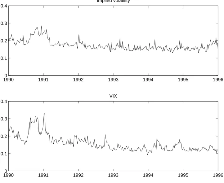
(17) 5. Empirical Results. This section presents the empirical results. We Þrst discuss the data, followed by an empirical evaluation of the model estimated under the physical measure using a historical series of stock returns. Subsequently we present estimation results obtained by estimating the risk-neutral version of the model using options data.. 5.1. Data. We conduct our empirical analysis using six years of data on S&P 500 call options, for the period 1990-1995. We apply standard Þlters to the data following Bakshi, Cao and Chen (1997). We only use Wednesday options data. Wednesday is the day of the week least likely to be a holiday. It is also less likely than other days such as Monday and Friday to be affected by day-of-the-week effects. For those weeks where Wednesday is a holiday, we use the next trading day. The decision to pick one day every week is to some extent motivated by computational constraints. The optimization problems are fairly time-intensive, and limiting the number of options reduces the computational burden. Using only Wednesday data allows us to study a fairly long time-series, which is useful considering the highly persistent volatility processes. An additional motivation for only using Wednesday data is that following the work of Dumas, Fleming and Whaley (1998), several studies have used this setup (see for instance Heston and Nandi (2000)). We perform a number of in-sample and out-of-sample experiments using the options data. We Þrst estimate the model parameters using the 1990-1992 data and subsequently test the model out-of-sample using the 1993 data. We also estimate the model parameters using the 1992-1994 data and subsequently test the model out-of-sample using the 1995 data. For both estimation exercises we use a volatility updating rule for the 500 days predating the Wednesday used in the estimation exercise. This volatility updating rule is initialized at the model’s unconditional variance. We also perform an extensive empirical analysis using return data. Ideally we would like to use the same sample periods for these estimation exercises, but it is well-known that it is difficult to estimate GARCH parameters precisely using relatively short samples on returns. We therefore use a long sample of returns (19631995) on the S&P 500. Table 1 presents descriptive statistics for the options data for 1990-1995 by moneyness and maturity. Panels A and B indicate that the data are standard. We can clearly observe the volatility smirk from Panel C and it is clear that the slope of the smirk differs across maturities. Descriptive statistics for different sub-periods (not reported here) demonstrate that the slope also changes across time, but that the smirk is present throughout the sample. The top panel of Figure 6 gives some indication of the pattern of implied volatility over time. For the 312 days of options data used in the empirical analysis, we present the average implied volatility of the options on that day. It is evident from Figure 6 that there is substantial 15.

(18) clustering in implied volatilities. It can also be seen that volatility is higher in the early part of the sample. The bottom panel of Figure 6 presents a time series for the 30-day at-the-money volatility (VIX) index from the CBOE for our sample period. A comparison with the top panel clearly indicates that the options data in our sample are representative of market conditions, although the time series based on our sample is of course a bit more noisy due to the presence of options with different moneyness and maturities.. 5.2. Empirical Results using Returns Data. Table 2 presents estimation results obtained using returns data for 1963-1995 for the physical model dynamics. We present results for three models: the GARCH(1,1) model (1), the component model (7) and the persistent component model (9). Almost all parameters are estimated signiÞcantly different from zero at conventional signiÞcance levels.13 In terms of Þt, the log likelihood values indicate that the Þt of the component model is much better than that of the persistent component model, which in turn Þts much better than the GARCH(1,1) model. The improvement in Þt for the component GARCH model over the persistent component GARCH model is perhaps somewhat surprising when inspecting the persistence of the component GARCH model. The persistence is equal to 0.996. It therefore would appear that equating this persistence to 1, as is done in the persistent component model, is an interesting hypothesis, but apparently modeling these small differences from one is important. It must of course be noted that the picture is more complex: while the persistence of the long-run component (ρ) is 0.990 for the component model as opposed to 1 for the ˜ is 0.644 versus persistent component model, the persistence of the short-run component (β) 0.764 and this may account for the differences in performance. Note that the persistence of the GARCH(1,1) model is estimated at 0.955, which is consistent with earlier literature. It is slightly lower than the estimate in Christoffersen, Heston and Jacobs (2004) and a bit higher than the average of the estimates in Heston and Nandi (2000). The ability of the models to generate richer patterns for the conditional versions of leverage and volatility of volatility is critical. For option valuation, the conditional versions of these quantities and their variation through time are just as important as the unconditional versions. The conditional versions of leverage and volatility of volatility are computed as follows. For the GARCH(1,1) model the conditional variance of variance is V art (ht+2 ) = Et [ht+2 − Et [ht+2 ]]2 = 2a21 + 4a21 c21 ht+1 13. (17). The standard errors are computed using the outer product of the gradient at the optimal parameter values.. 16.

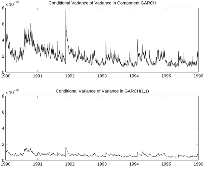
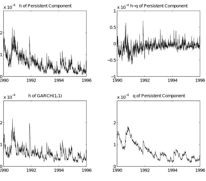
(19) and the leverage effect can be deÞned as Covt (ln (St+1 ) , ht+2 ) = Et [(ln (St+1 ) − Et [ln (St+1 )]) (ht+2 − Et [ht+2 ])] hp ³ í p 2 = Et ht+1 zt+1 a1 zt+1 − 2a1 c1 zt+1 ht+1 − a1. (18). = −2a1 c1 ht+1. The conditional variance of variance in the component model is V art (ht+2 ) = 2 (α + ϕ)2 + 4 (γ 1 α + γ 2 ϕ)2 ht+1. (19). and the leverage effect in the component model is Covt (ln (St+1 ) , ht+2 ) = −2 (γ 1 α + γ 2 ϕ) ht+1. (20). Figures 7 and 8 present the conditional leverage and conditional variance of variance for the GARCH(1,1) model and the component model over the option sample 1990-1995 using the MLE parameter values in Table 2. It can be clearly seen that the level as well as the time-series variation in these critical quantities are fundamentally different between the two models. In Figure 7 the leverage effect is much more volatile in the component model and it takes on much more extreme values on certain days. In Figure 8 the variance of variance in the component model is in general much higher than in the GARCH(1,1) model and it also more volatile. Thus the more ßexible component model is capable of generating not only more ßexible term structures of variance, it is also able to generate more skewness and kurtosis dynamics which are key for explaining the variation in index options prices. Table 2 also presents some unconditional summary statistics for the different models. The computation of these statistics deserves some comment. For the GARCH(1,1) model and the component model, the unconditional versions of the volatility of volatility are computed using the estimate for the unconditional variance in the expressions for the conditional moments (17) and (19). For the persistent component model, the unconditional volatility and the unconditional variance of variance are not deÞned. To allow a comparison of the unconditional leverage for all three models, we report the moments in (17) and (19) divided by ht+1 . While the unconditional volatility of the GARCH(1,1) model (0.137) is very similar to that of the component GARCH model (0.141), the leverage and the variance of variance of the component GARCH model are larger in absolute value than those of the GARCH(1,1) model. The leverage for the persistent component model is of the same order of magnitude as that of the component model. We previously discussed Figures 1-4, which emphasize other critical differences between the models. These Þgures are generated using the parameter estimates in Table 2. Figures 1 and 2 indicate that for the GARCH(1,1) model, forecasted model volatility reverts much more quickly towards the unconditional volatility over long-maturity options’ lifetimes than 17.

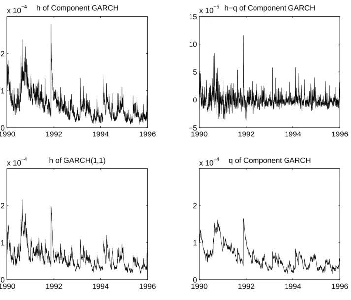
(20) is the case for the component model. Figures 3 and 4 demonstrate that the effects of shocks are much longer lasting in the component model because of the parameterization of the long-run component. As a result current shocks and the current state of the economy have a much more profound impact on the pricing of maturity options across maturities. Figures 9 and 10 give another perspective on the component models’ improvement in performance over the benchmark GARCH(1,1) model. These Þgures present the sample path for volatility in all three models, as well as the sample path for volatility components for the component model and persistent component model. In each Þgure, the sample path is obtained by iterating on the variance dynamic starting from the unconditional volatility 500 days before the Þrst volatility included in the Þgure, as is done in estimation. Initial conditions are therefore unlikely to affect comparisons between the models in these Þgures. Figure 9 contains the results for the component model. The overall conclusion seems to be that the mean zero short run component in the top-right panel adds short-horizon noise around the long-run component in the bottom-right panel. This results in a volatility dynamic for the component model in the top-left panel that is more noisy than the volatility dynamic for the GARCH(1,1) model in the bottom-left panel. The more noisy sample path in the top-left panel is of course conÞrmed by the higher value for the variance of variance in Table 2. This increased ßexibility results in a better Þt. The results for the permanent component model in Figure 10 conÞrm this conclusion, even though the sample paths for the components in Figure 10 look different from those in Figure 9.14. 5.3. Empirical Results using Options Data. Tables 3-10 present the empirical results for the option-based estimates of the risk-neutral parameters. We present four sets of results. Table 3 presents results for parameters estimated using options data for 1990-1992 using all option contracts in the sample. Note that the shortest maturity is seven days because options with very short maturities were Þltered out. Table 4 contains results for 1990-1992 obtained using options with more than 80 days to maturity, because we expect the component models to be particularly useful to model options with long maturities. Tables 5 and 6 present results obtained using options data for 1992-1994, using all contracts and contracts with more than 80 days to maturity respectively. When using the 1990-1992 sample in estimation, we test the model out-of-sample using data for 1993. When using the 1992-1994 sample in estimation, we test the model out-of-sample using 1995 data. Tables 7-10 present results for the two in-sample and two out-of-sample periods by moneyness and maturity. In all cases we obtain parameters by minimizing the 14. The Þgures presented so far have been constructed from the return-based MLE estimates in Table 2. Below we will present four new sets of (risk-neutral) estimates derived from observed option prices. In order to preserve space we will not present new versions of the above Þgures from these estimates. The option-based estimates imply Þgures which are qualitatively similar to the return-based Þgures presented above.. 18.

(21) dollar mean squared error $MSE =. ¢ 1 X¡ D M 2 Ci,t − Ci,t NT t,i. D M is the market price of option i at time t, Ci,t is the model price, and NT = where Ci,t. (21) T P. Nt .. t=1. T is the total number of days included in the sample and Nt the number of options included in the sample at date t. The parameters in Tables 3-6 are found by applying the nonlinear least squares (NLS) estimation techniques on the $M SE expression in (21). In the GARCH(1,1) case the implementation is simple: the NLS routine is called with a set of parameter starting values. The variance dynamic in (1) is then used to update the variance from one Wednesday to the next and the GARCH(1,1) option valuation formula from Heston and Nandi (2000) is used to compute the model prices on each Wednesday. In the component models an extra step is needed. Here the NLS routine is called with starting values for the component model, but the component model is converted to a GARCH(2,2) structure inside the optimization routine using (14). The implied GARCH(2,2) model is now used to update variance from Wednesday to Wednesday using (13) and to price options on each Wednesday using the option valuation formula in (16). Note that the NLS routine is thus optimizing the $M SE over the component parameters and not over the implied GARCH(2,2) parameters, which enforces the component structure throughout the optimization. The component structure is again useful both for the interpretation of the model and in implementation where reasonable starting values must be found.15 In Table 3 we present results for the 1990-1992 period (in-sample) and the 1993 period (out-of-sample). The standard errors indicate that almost all parameters are estimated signiÞcantly different from zero.16 There are some interesting differences with the parameters estimated from returns in Table 2, but the parameters are mostly of the same order of magnitude. This is also true for critical determinants of the models’ performance, such as unconditional volatility, leverage and volatility of volatility. It is interesting to note that in both tables the persistence of the GARCH(1,1) model and the component GARCH model is close to one. This of course motivates the use of the persistent component model, where the persistence is restricted to be one. Note also that the persistence of the short-run components and the long-run components is not dramatically different from Table 2. In the in-sample period, the RMSE of the component model is 90.0% of that of the benchmark GARCH(1,1) 15. Recall that the risk neutral GARCH process used in option valuation uses the parameterization c∗i = ci + λ + 0.5 so that ci and λ are not separately identiÞed. We therefore simply set λ equal to the MLE estimate from Table 2 for the respective models and do not report on it in Tables 3-6. This procedure identiÞes ci which in turns identiÞes the component model parameters. 16 The standard errors are again computed using the outer product of the gradient at the optimum.. 19.

(22) model. For the out-of-sample period, it is 76.5%. For the persistent component model, this is 94.5% and 96.6% respectively. Table 4 conÞrms that the same results obtain when estimating the models using only long-maturity options. Tables 5 and 6 present the results for the 1992-1994 period (in-sample) and the 1995 period (out-of-sample). The results largely conÞrm those obtained in Tables 3 and 4. The most important difference is that the in-sample and out-of-sample performance of the component model is even better relative to the benchmark, as compared with the results in Tables 3 and 4. For the 1992-1994 in-sample period, the component model’s RMSE is 76.9% of that of the GARCH(1,1) model in Table 5 and 73.1% in Table 6. For the 1995 out-of-sample period, this is 78.4% and 62.3% respectively. The performance of the persistent component model in some cases does not improve much over the performance of the GARCH(1,1) model, and in other cases its performance is actually worse than that of the benchmark. Another interesting difference with Tables 3 and 4 is that in Tables 5 and 6, the persistence of the short-run component is much higher. Finally note that the persistence of the GARCH(1,1) process in Table 5 is lower than in Table 3 but in line with the MLE estimate in Table 2. We conclude from Tables 3-6 that the performance of the component GARCH model is very impressive. Its RMSE is between 62.3% and 92.4% of the RMSE of the benchmark GARCH(1,1) model. The performance of the persistent component model is less impressive, both in-sample and out-of-sample.. 5.4. Discussion. It must be emphasized that this improvement in performance is remarkable and to some extent surprising. The GARCH(1,1) model is a good benchmark which itself has a very solid empirical performance (see Heston and Nandi (2000)). The model captures important stylized facts about option prices such as volatility clustering and the leverage effect (or equivalently negative skewness). When estimating models from option prices, Christoffersen and Jacobs (2004) Þnd that GARCH models with richer parameterizations do not improve the model Þt out-of-sample. Christoffersen, Heston and Jacobs (2004) Þnd that a GARCH model with non-normal innovations improves the model’s Þt in-sample and for short out-ofsample horizons, but not for long out-of-sample horizons.17 The performance of the benchmark GARCH(1,1) model can also be judged by considering the performance of its continuous-time limit, the Heston (1993) model, even though one must keep in mind that these limit results are somewhat tenuous (Corradi (2000)). Most of the continuous-time literature has attempted to improve the performance of the Heston (1993) model by adding to it (potentially correlated) jumps in returns and volatility. The empirical 17. Hsieh and Ritchken (2000) contains a discussion on the empirical performance of the HN GARCH(1,1) model vis-a-vis the performance of the more traditional GARCH model of Duan (1995).. 20.

(23) Þndings in this literature have been mixed. In general jumps in returns and volatility improve option valuation when parameters are estimated using historical time series of returns, but usually not when parameters are estimated using the cross-section of option prices (see for example Andersen, Benzoni and Lund (2002), Bakshi, Cao and Chen (1997), Bates (1996, 2000), Chernov, Gallant, Ghysels and Tauchen (2003), Eraker, Johannes and Polson (2003), Eraker (2004) and Pan (2002)). In a recent paper, Broadie, Chernov and Johannes (2004) use a long data set on options and an estimation technique that uses returns data and options data and Þnd evidence of the importance of some jumps for pricing. Carr and Wu (2004) and Huang and Wu (2004) model a different type of jump process and Þnd that they are better able to Þt options out-of-sample. Finally, Duan, Ritchken and Sun (2002) Þnd that adding jumps to discrete-time models leads to a signiÞcant improvement in Þt. Adding jumps or fat-tailed shocks to our model may therefore further improve the Þt. In summary, the option valuation literature is developing rapidly and it is not possible to convincingly judge the importance of some recent developments at this point. We merely want to emphasize that although the GARCH(1,1) may not be the best performing model in the literature, there are no other models available that spectacularly outperform it in- and out-of-sample. Given its parsimony, the GARCH(1,1) is therefore an excellent benchmark for our empirical study. It models a number of important issues such as volatility clustering and negative skewness that are deemed critical for option valuation, and there is not yet consensus regarding the empirical relevance of more richly parameterized models. By choosing GARCH(1,1) as a reference point we set a high standard in terms of empirical performance and parsimony. Because of the performance of this model in other studies, in our opinion the improvement of our model over GARCH(1,1) is spectacular. Tables 7-10 present results by moneyness and maturity. To save space we only report for the samples that include all options. Note that the tables contain information on MSEs, not RMSEs. In each table, Panel A contains the MSE for the GARCH(1,1) model. To facilitate the interpretation of the table, panels B and C contain MSEs that are normalized by the corresponding MSE for the GARCH(1,1) model. It is clear that an overall MSE which is not too different across the three models as in Table 3 can mask large differences in the models’ performance for a given moneyness/maturity cell. Inspection of the out-of-sample results in Tables 8 and 10 is very instructive. The overwhelming conclusion is that the improved out-of-sample performance of the component models is due to the improved valuation of long-maturity options. This is perhaps not surprising given the differences in the impulse response functions discussed above. Figure 11 graphically represents some related information. For different moneyness bins, we Þrst compute the average Black-Scholes implied volatility for all the options in our sample. Subsequently we compute implied volatilities based on model prices and also average this for all options in the sample. Note that while the implied volatility Þt is not perfect, the component model matches the volatility smirk better than the two other models. Figures 12 and 13 evaluate the performance of the three models along a different dimen21.

(24) sion, by presenting average weekly bias (average observed market price less average observed model price) over the 1990-1993 and 1992-1995 sample periods respectively. The bias seems to be more highly correlated across models in the 1990-1993 sample. In the 1993-1995 sample, the persistent component model in particular has a markedly different Þt from the two other models. The most important conclusion is that the improved performance of the component model does not derive from any particular sample sub-period: the bias of the component GARCH model is smaller than that of the GARCH(1,1) model in most weeks.. 6. Conclusion and Directions for Future Work. This paper presents a new option valuation model based on the work by Engle and Lee (1999) and Heston and Nandi (2000). The new variance component model has an empirical performance which is signiÞcantly better than that of the benchmark GARCH (1,1) model, in-sample as well as out-of-sample. This is an important Þnding because the literature has demonstrated that it is difficult to Þnd empirical models that improve on the GARCH(1,1) model or its continuous-time limit. The improved performance of the model is due to a richer parameterization which allows for improved joint modeling of long-maturity and shortmaturity options. This parameterization can capture the stylized fact that shocks to current conditional volatility impact on the forecast of the conditional variance up to a year in the future. Given that the estimated persistence of the model is close to one, we also investigate a special case of our model in which shocks to the variance never die out. The performance of the persistent component model is satisfactory in some dimensions, but it is strictly dominated by the component model. Note that this is not a trivial Þnding: even though the persistent component model is nested by the component model, a more parsimonious model can easily outperform a more general one out-of-sample. This is not the case here. Given the success of the proposed model, a number of further extensions to this work are warranted. First, the empirical performance of the model should of course be validated using other datasets. In particular, it would be interesting to test the model using LEAPS data, because the model may excel at modeling long-maturity LEAPS options. In this regard a direct comparison between component and fractionally integrated volatility models may be interesting. It could also be useful to combine the stylized features of the model with other modeling components that improve option valuation. One interesting experiment could be to replace the Gaussian innovations in this paper by a non-Gaussian distribution in order to create more negative skewness in the distribution of equity returns. Combining the model in this paper with the inverse Gaussian shock model in Christoffersen, Heston and Jacobs (2004) may be a viable approach. Finally, in this paper we have proposed a component model that gives a closed form solution using results from Heston and Nandi (2000) who rely on an affine GARCH model. We believe that this is a logical Þrst step, but the affine structure of the model may be restrictive in ways that are not immediately apparent. It 22.

(25) may therefore prove worthwhile to investigate non-affine variance component models.. 6.1. Appendix A. This appendix computes the autocorrelation functions (ACFs) for the innovation terms in 2 the GARCH(1,1) and component models. DeÞning ε2t+1 = zt+1 ht+1 , the ACF is in general given by Covt (ε2t+1 , ht+k ) Corrt (ε2t+1 , ε2t+k ) = Corrt (ε2t+1 , ht+k ) = q £ ¤p V art ε2t+1 V art [ht+k ]. (A1). Using the expression for the GARCH(1,1) dynamic from (10) ³ ´ p ¡ ¢ 2 2 2 2 ˜ ht+1 = σ + b1 ht − σ + a1 (zt − c1 ht ) − (1 + c1 ht ) σ2 =. w + a1 1 − ˜b1. ˜b1 = a1 c2 + b1 1. we have the following pieces constituting (A1) Covt (ε2t+1 , ht+k ) = 2˜bk−2 1 a1 ht+1 £ 2 ¤ V art εt+1 = 2h2t+1 Ã !2 k ³ ´2 X ˜bk−1 1 − 1 ˜bk−i a2 (2 + 4c2 Et [ht+i−1 ]) + 2 (w + a1 ) V art [ht+k ] = 3 + ˜bk−1 1 1 1 1 ht+1 ˜ 1 − b 1 i=2 2 Et [ht+i−1 ] = σ + ˜bi−2 (ht+1 − σ 2 ) 1. The component variance dynamic is ˜ (ht − qt ) + αv1,t ht+1 = qt+1 + β qt+1 = ω + ρqt + ϕv2,t with ³ p ´2 zt − γ 1 ht − (1 + γ 21 ht ) ³ p ´2 = zt − γ 2 ht − (1 + γ 22 ht ). v1,t = v2,t. 23.

(26) and the elements of (A1) are given by ˜ k−2 α + ρk−2 ϕ)ht+1 Covt (ε2t+1 , ht+k ) = 2(β £ ¤ V art ε2t+1 = 2h2t+1 ¶ k µ ³ ´2 ³ k−i ´2 X k−i k−i k−i e α+ρ ϕ +4 β e αγ 1 + ρ ϕγ 2 Et [ht+i−1 ] + V art [ht+k ] = 3 2 β i=2. µ. ¶2 1 − ρk−1 k−1 k−1 2 ω + ρ qt+1 + β (ht+1 − qt+1 ) 1−ρ ³ ´ ω i−2 i−2 ω ˜ + β (ht+1 − qt+1 ) + ρ Et [ht+i−1 ] = qt+1 − 1−ρ 1−ρ. 6.2. Appendix B. The mapping between the GARCH(2,2) and the component model given in (14) can be inverted to solve for the component parameters implied by a given GARCH(2,2) speciÞcation. We get the following solution a1 b21 + 4a1 b2 + 2a21 b1 c21 + a31 c41 + 4a1 a2 c22 2a2 + a1 b1 + a21 c21 √ − 2A 2 A a1 b21 + 4a1 b2 + 2a21 b1 c21 + a31 c41 + 4a1 a2 c22 2a2 + a1 b1 + a21 c21 √ + ϕ = 2A 2 A ³ √ ´ e = 1 b1 + a1 c2 − A β 1 2 ³ √ ´ 1 ρ = b1 + a1 c21 + A 2 e 2 + αρc2 − αβc e 1 − βϕc e 1 βϕc γ1 = e α(ρ − β) e 2 − αρc2 αρc1 + ρϕc1 − βϕc γ2 = e ϕ(ρ − β) α = a1 −. where. A = (b1 + a1 c21 )2 + 4(b2 + a2 c22 ). e ϕ, and ρ are real and Þnite as long as A > 0. Notice that α, β, e and ρ above are the roots of the polynomial Notice that the solutions for β Y 2 − (b1 + c21 a1 )Y − (b2 + c22 a2 ). Recall now the GARCH(2,2) process ³ ³ ´2 p ´2 p ht+1 = w + b1 ht + b2 ht−1 + a1 zt − c1 ht + a2 zt−1 − c2 ht−1 24. (B1).

(27) which can be written p p ¡ ¡ ¢ ¡ ¢ ¢ 2 ht+1 1 − b1 + a1 c21 L − b2 + a2 c22 L2 = w + a1 zt2 + a1 c1 ht zt + a2 zt−1 + a2 c2 ht−1 zt−1 where L is the lag operator. Nelson and Cao (1992) and Bougerol and Picard (1992) show that the roots of ¢ ¡ ¢ ¡ 1 − b1 + a1 c21 L − b2 + a2 c22 L2. (B2). need to be real and lie outside the unit circle in order for the variance to be stationary. e and ρ which are the roots of (B1) are the inverse of the roots of (B2). Notice that β e Therefore, β < 1 and ρ < 1 are required for the variance to be stationary in the GARCH(2,2) and the implied component model. The upshot is that the stationarity requirements imposed on the model are much easier to implement and monitor when the component structure is used.. 6.3. Appendix C. This appendix presents the moment generating function (MGF) for the GARCH(p,q) process used in this paper and in Heston and Nandi (2000). We Þrst derive the MGF of a GARCH(2,2) ³ ³ ´2 p ´2 p ht+1 = w + b1 ht + b2 ht−1 + a1 zt − c1 ht + a2 zt−1 − c2 ht−1. as an example and then generalize it to the case of the GARCH(p,q). Let xt = log(St ). For convenience we will denote the conditional generating function of St (or equivalently the conditional moment generating function (MGF) of xT ) by ft instead of the more cumbersome f (t; T, φ) (C1) ft = Et [exp(φxT )] We shall guess that the MGF takes the log-linear form. We again use the more parsimonious notation At to indicate A(t; T, φ). ³ ´ p ft = exp φxt + At + B1t ht+1 + B2t ht + Ct (zt − c2 ht )2 (C2). We have. h ³ í p ft = Et [ft+1 ] = Et exp φxt+1 + At+1 + B1t+1 ht+2 + B2t+1 ht+1 + Ct+1 (zt+1 − c2 ht+1 )2 (C3) Since xT is known at time T, equations (A1) and (A2) require the terminal condition AT = BiT = CT = 0 25.

(28) Substituting the dynamics of xt into (C3) and rewriting we get  ´2 ³ p φ(xt + r) + (B1t+1 a1 + Ct+1 ) zt+1 − (ct+1 − 2(B1t+1 aφ1 +Ct+1 ) ) ht+1 +  √ 2  A + B w + B b h + B a (z − c ht ) ! + t+1 1t+1 1t+1 2 t 1t+1 2 t 2  Ã ft = Et exp  φ2  φλ + B1t+1 b1 + B2t+1 + (φct+1 − 4(B1t+1 a1 +C1t+1 ) )+ ht+1 (B1t+1 a1 c21 + Ct+1 c22 ) − ct+1 (B1t+1 a1 c1 + Ct+1 c2 ) where ct+1 =.      . (C4). B1t+1 a1 c1 + Ct+1 c2 B1t+1 a1 + Ct+1. and we have used ¶2 µ p φ (B1t+1 a1 + Ct+1 ) zt+1 − (ct+1 − ) ht+1 2(B1t+1 a1 + Ct+1 ) p p = B1t+1 a1 (zt+1 − c1 ht+1 )2 + Ct+1 (zt+1 − c2 ht+1 )2 µ ¶ p φ2 +zt+1 φ ht+1 + −φct+1 + ht+1 4(B1t+1 a1 + Ct+1 ) ¡ ¢ − B1t+1 a1 c21 + Ct+1 c22 − ct+1 (B1t+1 a1 c1 + Ct+1 c2 ) ht+1. Using the result. in (C4) we get . £ ¤ 1 E exp(x(z + y)2 ) = exp(− ln(1 − 2x) + ay 2 /(1 − 2x)) 2. (C5).  φ(xt + r) + At+1 + B1t+1 w − 12 ln(1 − 2B1t+1 a1 − 2Ct+1 )+ φ (B1t+1 a1 +Ct+1 )(ct+1 − 2(B )2  √  1t+1 a1 +Ct+1 )  B1t+1 b2 ht + B1t+1 a2 (zt − c2 ht )2 + ht+1 +  1−2B a −2C )   1t+1 1 t+1 Ã ! ft = exp   φ2 φλ + B1t+1 b1 + B2t+1 + (φct+1 − 4(B1t+1 a1 +Ct+1 ) ) + ...   ht+1 2 2 (B1t+1 a1 c1 + Ct+1 c2 ) − ct+1 (B1t+1 a1 c1 + Ct+1 c2 ) (C6) Matching terms on both sides of (C6) and (C2) gives At = At+1 + φr + B1t+1 w −. 1 ln(1 − 2B1t+1 a1 − 2Ct+1 ) 2. ¡ ¢ B1t = φλ + B1t+1 b1 + B2t+1 + B1t+1 a1 c21 + Ct+1 c22. 1/2φ2 + 2 (B1t+1 a1 c1 + Ct+1 c2 ) (B1t+1 a1 c1 + Ct+1 c2 − φ) + 1 − 2B1t+1 a1 − 2Ct+1 26.

(29) B2t = B1t+1 b2 Ct = B1t+1 a2 where we have used the fact that φ2 − ct+1 (B1t+1 a1 c1 + Ct+1 c2 ) 4(B1t+1 a1 + Ct+1 ) (B1t+1 a1 + Ct+1 )(ct+1 − 2(B1t+1 aφ1 +Ct+1 ) )2. φct+1 − +. 1 − 2B1t+1 a1 − 2Ct+1 1/2φ + 2 (B1t+1 a1 c1 + Ct+1 c2 ) (B1t+1 a1 c1 + Ct+1 c2 − φ) = 1 − 2B1t+1 a1 − 2Ct+1 2. The case of GARCH(p,q) follows the same logic but is more notation-intensive. DeÞne two k × k upper-triangle matrices Zt = {Zij,t } and Ct = {Cij,t }, where ³ ´2 p for j + i ≤ q Zij,t = zt−i+1 − cj+i ht−i+1 for j + i > q. = 0. The moment generating function ft is assumed to be of the log-linear form µ ¶ p P 0 ft = exp φxt + At + Bit ht+2−i + I (Ct · ×Zt )I i=1. where I is a k × 1 vector of ones and k = q − 1. ·× represents element by element multiplication. After algebra similar to (C1)-(C6), we derive the following results: At = At+1 + φr + B1t+1 w −. B1t = φλ + B1t+1 b1 + B2t+1 +. Ã. q−1 P 1 ln(1 − 2B1t+1 a1 − 2 C1j,t+1 ) 2 j=1. B1t+1 a1 c21 +. q−1 X. C1j,t+1 c2j+1. j=1. !. +. ³ ´³ ´ P Pq−1 1/2φ2 + 2 B1t+1 a1 c1 + q−1 C c B a c + C c − φ 1j,t+1 j+1 1t+1 1 1 1j,t+1 j+1 j=1 j=1 Pq−1 1 − 2B1t+1 a1 − 2 j=1 C1j,t+1. for i = 2...p. Bit = B1t+1 bi + Bi+1t+1 27.

(30) for i = 1...k Cij,t = B1t+1 ai+1 = Ci+1j−1,t+1 = 0. for j = 1 and j + i ≤ q for j 6= 1 and j + i ≤ q for j + i > q. and AT = BiT = CT = 0. 6.4. Appendix D. This appendix derives the moment generating function for the component model directly. The component GARCH process is given by (7) ³ ´ p 2 2 ˜ ht+1 = qt+1 + β (ht − qt ) + α (zt − γ 1 ht ) − (1 + γ 1 ht ) ³ ´ p qt+1 = ω + ρqt + ϕ (zt − γ 2 ht )2 − (1 + γ 22 ht ). We shall again guess that the moment generating function has the log-linear form ft = exp[φxt + At;T,φ + B1t;T,φ (ht+1 − qt+1 ) + B2t;T,φ qt+1 ]. (D1). We have the terminal condition AT ;T,φ = BiT ;T,φ = 0. Applying the law of iterated expectations to ft;T,φ ,we get ft = Et [ft+1 ] = Et exp (φxt+1 + At+1;T,φ + B1t+1;T,φ (ht+2 − qt+2 ) + B2t+1;T,φ qt+2 ) Substituting the dynamics of xt gives p µ ¶ φ(xt + r) + φλht+1 + φ ht+1 zt+1 + At+1;T,φ + B1t+1;T,φ (ht+2 − qt+2 )+ ft = Et exp B2t+1;T,φ qt+2 p   zt+1 + At+1;T,φ + ³ φ(xt + r) + φλht+1³ + φ ht+1p ´´   B1t+1;T,φ β˜ (ht+1 − qt+1 ) + α (zt+1 − γ 1 ht+1 )2 − (1 + γ 21 ht+1 ) +  = Et exp    ³ ´´ ³ p B2t+1;T,φ ω + ρqt+1 + ϕ (zt+1 − γ 2 ht+1 )2 − (1 + γ 22 ht+1 )  φ(xt + r) + φλht+1 + At+1;T,φ + B1t+1;T,φ β˜ (ht+1 − qt+1 ) +  B2t+1;T,φ (ω + ρqt+1 ) − (aB1t+1;T,φ + ϕB2t+1;T,φ )+  ³ ´2  aγ 1 B1t+1;T,φ +ϕγ 2 B2t+1;T,φ −0.5φ p = Et exp  (aB + ϕB ) + z − h − 1t+1;T,φ 2t+1;T,φ t+1 t+1 (aB1t+1;T,φ +ϕB2t+1;T,φ )  2 (aγ 1 B1t+1;T,φ +ϕγ 2 B2t+1;T,φ −0.5φ) ht+1 (aB1t+1;T,φ +ϕB2t+1;T,φ ) 28.      .

(31) Using (C5) we get .   ft = Et exp  . φ(xt + r) + At+1;T,φ − (aB1t+1;T,φ + ϕB2t+1;T,φ ) −1/2 ln (1 − 2aB1t+1;T,φ − 2ϕB2t+1;T,φ ) + B2t+1;T,φ ω+ B³1t+1;T,φ β˜ (ht+1 − qt+1 ) + B2t+1;T,φ ρq ´t+1 )+ aγ 1 B1t+1;T,φ +ϕγ 2 B2t+1;T,φ −0.5φ λφ + 2 1−aB1t+1;T,φ −ϕB2t+1;T ,φ ht+1. Matching terms on both sides of (D2) and (D1) gives.     . (D2). At;T,φ = At+1;T,φ − (aB1t+1;T,φ + ϕB2t+1;T,φ ) − 1/2 ln (1 − 2aB1t+1;T,φ − 2ϕB2t+1;T,φ ) + B2t+1;T,φ ω aγ B1t+1;T,φ + ϕγ 2 B2t+1;T,φ − 0.5φ B1t;T,φ = B1t+1;T,φ β˜ − 1/2φ + 2 1 1 − aB1t+1;T,φ − ϕB2t+1;T,φ aγ 1 B1t+1;T,φ + ϕγ 2 B2t+1;T,φ − 0.5φ B2t;T,φ = B2t+1;T,φ ρ − 1/2φ + 2 1 − aB1t+1;T,φ − ϕB2t+1;T,φ. 29.