HAL Id: hal-01057072
https://hal.archives-ouvertes.fr/hal-01057072
Submitted on 21 Aug 2014
HAL is a multi-disciplinary open access
archive for the deposit and dissemination of
sci-entific research documents, whether they are
pub-lished or not. The documents may come from
teaching and research institutions in France or
abroad, or from public or private research centers.
L’archive ouverte pluridisciplinaire HAL, est
destinée au dépôt et à la diffusion de documents
scientifiques de niveau recherche, publiés ou non,
émanant des établissements d’enseignement et de
recherche français ou étrangers, des laboratoires
publics ou privés.
Price Competition between Road Side Units Operators
in Vehicular Networks
Vladimir Fux, Patrick Maillé, Matteo Cesana
To cite this version:
Vladimir Fux, Patrick Maillé, Matteo Cesana. Price Competition between Road Side Units Operators
in Vehicular Networks. Networking 2014 : IFIP Networking conference, Jun 2014, Trondheim, Norway.
�10.1109/IFIPNetworking.2014.6857112�. �hal-01057072�
Price Competition between Road Side Units
Operators in Vehicular Networks
Vladimir Fux, Patrick Maill´e
Institut Mines-Telecom/Telecom Bretagne - IRISA 2, rue de la Chataigneraie
35576 Cesson-S´evign´e Cedex - France Email:{name.surname}@telecome-bretagne.eu
Matteo Cesana
Dipartimento di Elettronica, Informazione e Bioingegneria Politecnico di Milano
Piazza Leonardo da Vinci, 32 - 20133 Milano - Italy Email:{name.surname}@polimi.it
Abstract—Vehicular networks, besides supporting safety-oriented applications, are nowadays expected to provide effec-tive communication infrastructure also for supporting leisure-oriented application including content sharing, gaming and In-ternet access on the move. This work focuses on Vehicle to Infras-tructure (V2I) scenarios, where multiple content providers own a physical infrastructure of Road Side Units (RSUs) which they use to sell contents to moving vehicles. Content provider/RSU owners compete by adapting their pricing strategies with the selfish objective to maximize their own revenues. We study the economics of the price competition between the providers by resorting to game theoretic tools. Namely, we formalize a simultaneous price game among the operators further studying the existence of Nash equilibria and their related quality in terms of Price of Anarchy and Price of Stability. The proposed game model is finally used to assess the impact onto the game equilibra of several practical factors including the vehicles’ willingness to pay, the traffic densities, and the configuration of the physical networks of RSUs.
I. INTRODUCTION
The constant increase in the number of cars traveling along the roads worldwide calls for effective means to improve the road safety and the efficiency of the overall transportation infrastructure. To this end, the research community, the in-dustries and the governments all over the world are investing much of their efforts and money on the development of integrated Intelligent Transportation Systems (ITS) based on wireless communication networks allowing vehicles, equip-ment on the road, service centers and intelligent sensors to exchange information in a prompt and cost effective way. In this scenario, vehicles are geared with wireless communication hardware, often referred to as On Board Units (OBUs), to sup-port communication with other vehicles (Vehicle-to-Vehicle, V2V) and with road infrastructure (Vehicle-to-Infrastructure, V2I). In this last case, the devices composing the roadside infrastructure are often called RoadSide Units (RSUs).
A broad classification of the applications which are enabled by vehicular networks can be found in [9] where a distinc-The project GreenEyes acknowledges the financial support of the Future and Emerging Technologies (FET) programme within the Seventh Framework Programme for Research of the European Commission, under FET-Open grant number:296676.
tion is made between applications targeting safety, transport efficiency, and information/entertainment. Safety applications include, as an example, collision warning services, transport efficiency application may include lane merging assistance, and navigation services, whereas information/entertainment application range from file sharing among vehicles to Internet access on the move.
In this work, we focus on the vehicle-to-infrastructure (V2I) communication paradigm for VANETs to support content distribution to moving vehicles. Namely, we consider the case where multiple content providers coexist and compete in a given geographical area. Each content provider owns a physical infrastructure of RSUs which she uses to sell contents to moving vehicles. Content provider/RSU owners compete by adapting their pricing strategies with the selfish objective to maximize their own revenues. In such a scenario, we ask ourselves the following simple question: if competing providers wish to select the pricing strategy in order to provide or collect data to/from passing vehicles, what kind of strategies should they follow? The answer is far from being trivial as it predictably depends on several factors including the vehicles’ willingness to pay, the traffic densities, the configuration of the physical networks of RSUs, and the strategic interaction among the content providers.
We tackle this problem by considering a basic model with a duopoly of competing content providers. We study the economics of the competition between the two providers by resorting to game theoretic tools [13], [18]. We first analyze the best-response strategies of each operator, and treat the case where both operator compete simultaneously on prices. We formally study the existence of Nash equilibria for the duopoly pricing game and their related quality in terms of Price of Anarchy.
The manuscript is organized as follows: Section II reviews the related literature in the field further highlighting the major novelties of the present work; in Section III, the reference network scenario and model are described. Section IV provides the analysis of the best response of one operator when the pricing strategy of the other is given, whereas the simultaneous pricing game is analyzed in Section V. Section VI concludes and indicates some directions for future work.
II. RELATED WORK
The design of efficient V2I and V2V networks has already attracted much attention within the research community. Most of the work generally targets the design and optimization of communication protocols to be used in vehicular networks. As an example, the optimization of V2I segment is targeted in [24] where the focus in on uplink and downlink packet scheduling techniques. Along the same lines, Yang et al. study in [22] the applicability and performance of IEEE 802.16 for the communication between groups of vehicles and an RSU.
V2V communications are addressed in [4], [12], [23]. In [4] a Medium Access Control (MAC) protocol is proposed to support reliable communication among vehicles. The work in [23] proposes a protocol framework to support the dissemi-nation of warning messages in V2V, whereas the use of V2V communications to support proactive data monitoring in urban environments in studied in [12].
In the field of V2I networks, besides the work on protocol design/optimization, it is worth mentioning the research field targeting the optimal design of the roadside infrastructure. In this case, the goal is to optimize the deployment of the RSUs with respect to specific objectives which are generally related to the coverage ratio of vehicles. Trullols et al. [20] propose three formulations for the the deployment problem as a Maximum Coverage Problem (MCP), Knapsack Problem (KP), and Maximum Coverage with Time Threshold Problem (MCTTP), respectively; heuristics based on local-search and greedy approaches are then introduce to get suboptimal solu-tions. Along the same lines, Cavalcante et al. [5] focus on the Maximum Coverage with Time Threshold Problem (MCTTP) and propose a genetic algorithm to solve it. Yan et al.. [21] study the very same RSU deployment problem in case the candidate sites for deployment are limited to the intersections between crossing roads. The interested reader may refer to [2] and references therein for a more comprehensive description on the general problem of RSU deployment. Different from the aforementioned work which assumes one central entity to optimize the RSU deployment, [6] studies the competitive scenario where different network operators compete in the deployment of their respective RSUs by resorting to a non-cooperative game. Spatial positioning games are also proposed in [1] for generic wireless access networks.
Game theory has been used to evaluate the strategic interac-tion between the different agents in vehicular networks [17]. In [16], the authors introduce a stochastic game among OBUs which compete to get service from shared RSUs. Nyiato et
al. propose in [15] a hierarchical game framework to capture the competition of different actors; besides OBUs and RSUs, the concept of Transit Service Provider (TSP) is used to model an entity which manages groups of vehicles and is in charge of minimizing the total cost to support streaming application to its vehicles while meeting the application QoS requirement. The available bandwidth at each RSU can be split in reserved bandwidth and on-demand bandwidth. OBUs make short-term decisions between on-demand and reserved
bandwidth (if available), TSPs decides what kind of bandwidth split to purchase from different RSUs along the road, whereas Network Service Providers (NSPs) owning RSUs set their price for on-demand bandwidth to maximize their revenues. Differently, in [19] a coalition formation game among RSU is analyzed, with the aim of better exploiting V2V communica-tions for data dissemination.
The matter of pricing in generic wireless access networks is largely debated in the literature. Reference [14] provides a nice overview on pricing problems in wireless networks, and further analyze a specific case where two wireless Internet service providers compete on prices, one owning a WiMAX-based in-frastructure and the other running a WiFi-based inin-frastructure. Differently from previously mentioned literature, in this work we focus on price competition between network operators for V2I networks, which is, to the best of our knowledge, a novel issue. Even if V2I networks bear some similarities with generic wireless access networks, there are distinctive features which make the pricing problem worth analyzing; in generic wireless access networks, the network operator competition is generally on the “common” users, that is, those users which fall in the coverage area of the competing network providers. In other words, there is actually a competition only if the coverage areas of the network providers (partially) overlap as in [14]. Users themselves tend to choose the network operator which maximizes some quality measure as in [8]. On the other side, in V2I networks competition may arise due to vehicles mobility even if the coverage areas of competing RSUs are not overlapping, since if a RSU does not serve a moving vehicle in its own coverage range, the very same user can be served later by competing operators.
III. MODEL
A. Usage scenario
We consider two Internet access providers (labeled by 1 and 2), competing to attract users on a stretch of a highway. They offer the possibility to access the Internet through Road Side Units, which allows cheaper or better QoS than the other available cellular networks. (Note that we ignore vehicle-to-vehicle communications in this paper.) We assume that each provider has already deployed one RSU –on different locations along the road–, and that both RSU are identical; we denote their individual goodput (or capacity) by c. (Note that this model easily extends to the case when providers own disjoint “connectivity regions”, each one made of several RSUs and with total service capacity c.)
Since both providers’ RSU are at different locations, vehi-cles taking the road in one direction first enter the coverage area of Provider1’s RSU, while those traveling in the opposite direction first see Provider 2. We denote by ⇢j,j = 1, 2 the
average number of commuters per time unit that first enter Provider j’s coverage area; they will cross the competitor’s coverage area afterwards (since we are considering only one road).
Each user wants to download data files, for an average volume per user (assumed independent of the travel direction)
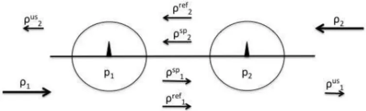
Fig. 1. Flows involved in the model: among the total potential demandρj
seeing Providerj first, we distinguish ρspj (demand from users agreeing to
paypj, but not served by this provider),ρrefj (demand from users refusing to
paypj) andρusj (demand unserved by any provider).
normalized to 1 without loss of generality; the potential demand (in volume) from users seeing Provider j first thus also equals ⇢j. In this paper, we treat those average loads
as static values, i.e. we do not model the time variations of the load. Moreover, we assume that the coverage area size of RSUs and the vehicles’ speed do not constrain the transfers: if a RSU’s capacity exceeds its (average) load, all requests are successfully served.
Each provider j = 1, 2 chooses the (flat-rate) price pj to
charge for the connection service. To model heterogeneity among users, we assume that only a proportion w(p) of users accept to pay a unit pricep for the service (this being independent of the download volume). As a result, if Provider j sets his price to pj, the users who first enter Provider j’s
service area generate a demand (again, per time unit, and treated as static) ofw(pj)⇢j. Note that we are assuming here
that users do not try to anticipate the price set by the next provider: when a user first sees an RSU access offer, she responds to it as if there were no other RSU afterwards.
Figure 1 summarizes that scenario in terms of demand flows. The total potential demand (volume per time unit) ⇢j from
users seeing Providerj can be decomposed into:
1) users accepting the price pj and being served by
Provider j;
2) users accepting the pricepjand being rejected due to the
RSU capacity limit (forming a spillover flow⇢spj heading to the competitor’s RSU);
3) and users refusing the price pj (forming a flow ⇢refj
heading to the competitor’s RSU).
The two latter flows then enter the coverage area of the competing provider, where they can be served or not. In the latter case, we denote the corresponding (unserved) demand by ⇢us
j . Note that we assume users keep the same
willingness-to-pay for the service when they enter the second RSU coverage area.
B. Mathematical formulation
We now give analytical expressions for the different demand components, using the RSU capacity c and the willingness-to-pay function w(·). In the whole paper, w(·) is assumed continuous and non-increasing, and such that w(0) = 1 and
w(pmax) = 0 for some pmax > 0. If the quality of the
alternative cellular access (say, 4G) is sufficient, the price pmax may be interpreted as the unit price for that cellular
service: above pmax, users have no interest to use an
RSU-based access.
The demand submitted to Provider j comes from three different types of users:
1) those seeing Provider j first, and accepting to pay the proposed pricepj, hence issuing a total demand
w(pj)⇢j;
2) those seeing Provider k 6= j (the competing provider) first, who refused to paypk but would accept the price
pj, forming a total demand level (smaller than⇢refk , and
null whenpk pj)
⇢k[w(pj) − w(pk)]+,
wherex+:= max(0, x) for x 2 R.
3) and those seeing Provider k first, who agreed to pay pk but were rejected because of Provider k’s limited
capacity, and who also agree to pay pj, for a total
demand min ✓ 1,w(pj) w(pk) ◆ ⇢spk,
where ⇢spk is the part of the demand w(pk)⇢k that is
spilled over by Providerk. The total demand⇢T
j(pj, pk) for Provider j then equals the
sum of the aforementioned components: ⇢T j(pj, pk) := w(pj)⇢j+ ⇢k[w(pj) − w(pk)]++ min ⇣ 1,w(pj) w(pk) ⌘ ⇢spk Note the dependance in both prices, although for simplicity we will sometimes just write⇢T
j when there is no ambiguity.
When the total demand at an RSU exceeds its capacity, some requests are rejected: we assume the RSU serves users up to its capacity level, and the rejected requests are selected randomly among all requests. This leads to an identical probability of success Pj for each request submitted to Provider j, that is
simply given by Pj= min 1, c ⇢T j ! (1) so that the served traffic at RSUj equals ⇢T
jPj= min(c, ⇢Tj).
Again, the probabilityPj depends on the price vector(pi, pj).
The corresponding revenue of Provider j is then
Rj= pjmin[c, ⇢Tj(pj, pk)]. (2)
The traffic⇢spj spilled over by Providerj (and that will then enter the competitor’s coverage area) also depends on both prices through the probabilityPj, and equals
with Pj = min 0 @1, c w(pj)⇢j+[w(pj)−w(pk)]+⇢k+min[1,w(pw(pjk))]⇢spk 1 A.
Remark that for a given price configuration (p1, p2), the
success probabilities P1 and P2 are the solution of a
fixed-point system, since the success probability Pj of Providerj
depends on the spillover demand ⇢spk and thus on Pk, that
itself depends on ⇢spj and hence on Pj. More specifically,
assuming without loss of generality thatp1≥ p2, those success
probabilities should satisfy 8 < : P1= min ⇣ 1,w(p c 1)(⇢1+⇢2)−w(p1)⇢2P2 ⌘ P2= min ⇣ 1,w(p c 2)(⇢1+⇢2)−w(p1)⇢1P1 ⌘ . (4)
Proposition 1: For any price vector(p1, p2), the system (4)
has a unique solution(P1, P2).
Proof: We again assume without loss of generality that p1≥ p2. Since the right-hand sides of the equations in (4) are
continuous in(P1, P2) and fall in the interval [0, 1], Brouwer’s
fixed-point theorem [10] guarantees the existence of a solution to the system.
To establish uniqueness, remark thatP2is uniquely defined
byP1through the second equation in (4), so(P1, P2) is unique
ifP1is unique. ButP1is a solution in[0, 1] of the fixed-point
equation x = g(x) with g(x) := min 0 @1, 1 a + b − b min⇣1, 1 a+b+✏−ax ⌘ 1 A, wherea =w(p1)⇢1 c ,b = w(p1)⇢2 c , and✏ = (w(p2)−w(p1))(⇢1+⇢2) c
are all positive constants; we also assume a > 0 and b > 0 otherwise the problem is trivial. As a combination of two func-tions for the form x 7! min⇣1,K1−K1 2x⌘, g is continuous, nondecreasing, strictly increasing only on an interval[0, ¯x] (if any) –it is in addition convex on that interval–, and constant for x ≥ ¯x (note we can have ¯x = 0 or ¯x ≥ 1).
Assume g(x) = x has a solution ˜x 2 (0, ¯x]. Then g is left-differentiable atx, and˜ g0 (˜x) = x˜ 2ab (a + b + ✏ − a˜x)2 ˜ x2a (a + b + ✏ − a˜x) (5) where we used the fact that x 1 (as a fixed point of˜ g). Moreover, since ˜x is in the domain where g is strictly increasing we have ⌘ := 1
a+b+✏−a˜x 1 on one hand, and
˜
x = 1
a+b−b⌘ on the other side. Their combination yieldsx ˜ 1 a
and finally
g0
(˜x) ˜x 1.
Remark also thatg0(˜x) < 1 if ˜x < 1. We finally use the fact
thatg(0) > 0 to conclude that the curve y = g(x) cannot meet the diagonal y = x more than once: assume two intersection pointsx˜1 < ˜x2, then g0(˜x1) < 1 thus the curves cross at ˜x1,
another intersection point x would imply g˜ 0(˜x
2) > 1 (recall
g is convex when strictly increasing), a contradiction. Hence the uniqueness of the fixed point and of the solution to (4).
We can also establish continuity properties for the solution of (4), which will be used in the remainder of this paper.
Proposition 2: The success probability pair(P1, P2) is
con-tinuous in the price profile(p1, p2).
Proof: For a given price profile (p1, p2), the solution
(P1, P2) of (4) can also be seen as a solution of the
mini-mization problem min (P1,P2)2[0,1]2 ✓ P1−min ✓ 1, c w(p1)(⇢1+⇢2) − w(p1)⇢2P2 ◆◆2 + ✓ P2−min ✓ 1, c w(p2)(⇢1+⇢2) − w(p1)⇢1P1 ◆◆2 , where the objective function is jointly continuous in(P1, P2)
and (p1, p2). From the Theorem of the Maximum [3], the
mapping of prices (p1, p2) into the corresponding set of
solutions(P1(p1, p2), P2(p1, p2)) is an upper hemicontinuous
correspondence. From the uniqueness result above, that corre-spondence is single-valued and hence continuous. We therefore have continuity for p1≥ p2 and for p2≥ p1 (exchanging the
roles of providers), hence continuity for all price profiles. IV. REVENUE-MAXIMIZING PRICE FOR A PROVIDER In this section we assume that providerk has already chosen his price, while provider j has to set his. We describe the revenue function of provider j for different scenarios, and provide an example when the willingness-to-pay function is linear.
In this whole section, we only consider prices p such that w(p) > 0, since a larger price would yield no revenue to the provider setting it.
We first establish a monotonicity result, that will be useful in the rest of the analysis.
Lemma 1: The total demand⇢T
j of providerj is a
continu-ous function of his price pj; that function is in addition
non-increasing while providerj is not saturated (i.e., while ⇢T j < c).
Proof: Recall that ⇢T
j(pj, pk) = w(pj)⇢j+ ⇢k[w(pj) − w(pk)]+
+ min (w(pk), w(pj)) ⇢k(1 − Pk).
The components of the first line are trivially continuous and non-increasing inpj with our assumptions on w(·).
The continuity of⇢T
j(pj, pk) follows from the continuity of
Pk in the price vector (pj, pk), established in the previous
section. To establish monotonicity, we distinguish two cases. • If pj pk, we show that the success probabilityPk is
non-decreasing inpj: applying System (4) (withk = 1, j = 2) we
get thatPkis the solution of the fixed-point equationx = g(x),
where the function g can be written as
g(x) = min 0 B @1, c w(pk)⇢k+w(pk)⇢j h 1− c w(pj)(⇢j+⇢k)−w(pk)⇢kx i+ 1 C A.
We then remark that, all else being equal, g(x) is non-decreasing inpj, so the solutionPkof the fixed-point equation
g(x) = x is also non-decreasing in pj.
As a result, when pk ≥ pj the component
min (w(pk), w(pj)) ⇢k(1 − Pk) decreases with pj, and
so does⇢T j. • If pk < pj, then we have ⇢T j(pj, pk) = w(pj)⇢j+ w(pj)⇢k(1 − Pk). When⇢T
k < c, then Pk = 1 and ⇢Tj is non-increasing inpj.
Now if⇢T
k> c then from System (4) (this time with k = 2,
j = 1), we have w(pk)(⇢j+ ⇢k) − w(pj)⇢jPj> c and ⇢T j(pj, pk) = w(pj)(⇢j+ ⇢k) +w(pj)⇢k c w(pk)(⇢j+ ⇢k) − w(pj)⇢jPj . Assuming that provider j is not saturated, Pj = 1 and thus
⇢T j = f (w(pj)) with f (x) := x(⇢j+ ⇢k) − x⇢k c w(pk)(⇢j+ ⇢k) − x⇢j . Butf is a non-decreasing function of x when x 2 [0, w(pk)]
andw(pk)(⇢j+ ⇢k) − x⇢j> c: differentiating we indeed get
f0(x) ⇢j+ ⇢k = 1 − ⇢kc w(pk) (w(pk)(⇢j+ ⇢k) − x⇢j)2 ≥ 1 − ⇢kw(pk) w(pk)(⇢j+ ⇢k) − x⇢j ≥ 1 − ⇢kw(pk) w(pk)(⇢j+ ⇢k) − w(pk)⇢j ≥ 0,
where we usedw(pk)(⇢j+ ⇢k) − x⇢j > c in the second line,
and x w(pk) in the last one. The non-increasingness of
⇢T
j = f (w(pj)) in pj then comes from that ofw(·).
A. Capacity saturation price
For further analysis, we define the capacity saturation price of a provider, that depends on the price of his competitor.
Definition 1: The capacity saturation price of providerj is pc
j(pk) := inf{p 2 [0, pmax] : ⇢Tj(p, pk) < c}.
Since⇢T
j(pmax, pk) = 0, for all pk we havepcj(pk) < pmax.
Additionally, Lemma 1 implies that if pc
j > 0, then
⇢T
j(pcj, pk) = c and pj pcj ) ⇢Tj ≥ c.
We now provide analytical expressions for that price, in the case when ⇢T
j(p, pk) ≥ c. In that case ⇢Tj(pcj) = c, hence pcj
satisfies 8 < : w(pj)⇢j+ ⇢k[w(pj) − w(pk)]++ min ⇣ 1,w(pj) w(pk) ⌘ ⇢spk = c, ⇢spk = w(pk)⇢k h[w(p k)−w(pj)]+⇢j+w(pk)⇢k−c [w(pk)−w(pj)]+⇢j+w(pk)⇢k i+ . (6) Let us define a generalized inverse ofw, as
W (q) := inf{p 2 [0, pmax] : w(p) < q}. (7)
Forq 1, W (q) is the maximum price that can be accepted by a proportionq of users.
Then the capacity saturation price can be computed as follows. (The proof is omitted due to space constraints.)
• If w(pk) min[c ⇢j, c ⇢k], then p c j = W ⇣c+w(p k)⇢k ⇢j+⇢k ⌘ . • If c ⇢k < w(pk) 2c ⇢j+⇢k, thenp c j = W ⇣ 2c ⇢j+⇢k ⌘ . • If c ⇢j < w(pk) 2c ⇢j+⇢k, thenp c j = W ⇣ c ⇢j ⌘ . • If w(pk) > 2c ⇢j+⇢k, then p c
j = W (x), with x the unique
solution in [0, w(pk)] of −x2⇢j+ x ✓ w(pk)(⇢j+ ⇢k) − c ⇢k− ⇢j ⇢j+ ⇢k ◆ − cw(pk) = 0.
B. Piece-wise expression of the revenue function
The revenue function of each provider j is continuous in his price (from the continuity of ⇢T
j and of Pj), and can be
expressed analytically on different segments.
1) When pj pcj(pk) (or ⇢Tj(pj) ≥ c when pcj(pk) > 0),
the RSU capacity of providerj is saturated, and thus his revenue is simply
Rj = pjc. (8)
This is the case in Figure 3 for pricespj below
approxi-mately2.5. Figure 5 shows that for these prices, provider j spills some flow over toward provider k.
Abovepc
j, provider j is not saturated anymore. Then if
the total demand⇢k(pcj, pk) of the competitor is strictly
belowc, we have a price range with no provider being saturated. In that case we have no spillover demand, and the revenue of providerj is:
Rj= pj2w(pj)⇢j+ [w(pj) − w(pk)]+⇢k3 .
Ifpc
j< pk, then we remark that necessarily⇢Tk(pk, pk)
c, i.e., we meet the price of the opponent provider before he gets saturated. Indeed, at(pc
j, pk) provider j does not
spill traffic over tok, thus ⇢T
k(pcj, pk) = ⇢kw(pk) (where
we also used the fact that w(pk) w(pcj)). From the
definition of pc
j, provider j is not saturated at (pk, pk),
so that ⇢T
k(pk, pk) = ⇢kw(pk) = ⇢Tk(pcj, pk) c.
Summarizing, we then have the two following segments. 2) If pc
j < pk and⇢Tk(pcj, pk) c, then for pj 2 [pcj, pk]
Rj= pj(w(pj)(⇢j+ ⇢k) − w(pk)⇢k) .
Remark that this segment is empty if pc
j ≥ pk or
⇢T
k(pcj, pk) ≥ c. Figure 5 illustrates that when pj is
between approximately2.5 and 4, provider j serves his own traffic and the one from the competitor who refused the pricepk but agrees to pay pj.
3) If ⇢T
k(pcj, pk) c, then for pj ≥ max(pcj, pk) we have
while providerk remains unsaturated: Rj = pjw(pj).
4) Now if⇢k(pcj, pk) > c, then provider k is saturated for
pj 2 [pcj, pmax] (which is easy to see since j has no
spillover traffic), and forpj 2 [pcj, pk] we have
Remark that this segment appears only when both providers can be simultaneously saturated, a case not occurring in the example we display here.
5) There may be a price of provider j larger than pk,
and above which the competitor gets saturated, so that provider j may serve part of the traffic spilled over by k. In that case the revenue of provider j is:
Rj= pj ✓ w(pj)⇢j+ w(pj) w(pk)⇢ sp k ◆ , (9) where ⇢spk = w(pk)⇢ (w(pk) − w(pj))⇢j+ w(pk)⇢k+ ⇢spj − c (w(pk) − w(pj))⇢j+ w(pk)⇢k+ ⇢spj . (10) Figure 6 shows that provider k gets saturated, and the spillover traffic is served partly by provider j as illustrated in Figure 5.
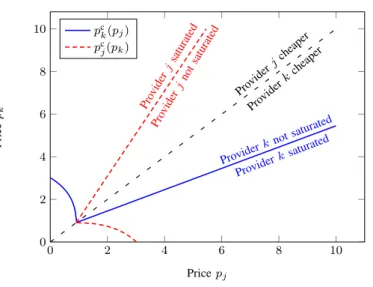
Figure 2 illustrates those different zones for the special case ⇢1 = ⇢2 = 11, c = 10, and w(p) = 1 − p/10. Figure 3
shows the corresponding different segments for Rj when
pk = 4, and Figure 4 for various prices pk of the competitor.
We observe that a revenue-maximizing price can belong to different segments, depending on the competitor’s price.
0 2 4 6 8 10 0 2 4 6 8 10 Provider k saturated Provider k notsaturated Provider kcheaper Provider jcheaper Pro vider jsaturated Pro vider jnot saturated Pricepj Price pk pc k(pj) pc j(pk)
Fig. 2. Capacity saturation prices, and the different zones where the
expressions of revenues vary.
V. PROVIDERS PRICING GAME
In this section we consider a non-cooperative game, where providers –the players– simultaneously choose their prices, trying to maximize their individual payoffs given by (2). Our aim is to find a Nash equilibrium (NE) of this game: a pair of prices(¯p1, ¯p2), such that no player could increase his revenue
by unilaterally changing his price. Further, we investigate the situation where providers would decide to cooperate, trying to maximize the sum of their individual revenues (as a monopoly would do). We analyze how much the providers lose in terms of total revenue by refusing to cooperate.
0 2 4 6 8 10 0 10 20 30 Providerj
saturated No providersaturated Competitorsaturated
Pro vider j cheaper Pro vider k cheaper Pricepj Re v enue
Fig. 3. Revenue of providerj as a function of his price pj, forpk = 4,
ρ1= ρ2= 11, c = 10 and w(p) =
10 −p
10 , illustrating the different segments.
0 2 4 6 8 10 0 10 20 30 40 Pricepj Re v enue pk= 3 pk= 4 pk= 5 pk= 8
Fig. 4. Revenue of providerj vs his price for different pk values, when
w(p) is linear. The different segments correspond to the zones delimited in
Figure 2 for each givenpk.
Below is a more formal definition of the Nash equilibrium in the pricing game.
Definition 2: A pair of prices(¯p1, ¯p2) is a Nash equilibrium
for the pricing game if
R1(¯p1, ¯p2) ≥ R1(p1, ¯p2) for all p12 (0, pmax],
R2(¯p1, ¯p2) ≥ R2(¯p1, p2) for all p22 (0, pmax].
Nash equilibria can be interpreted as predictions for the outcome of the competition between selfish entities, assumed rational and taking decisions simultaneously.
A. The case of large capacities
We first consider here that RSUs capacities are larger than the users flows (c ≥ ⇢j + ⇢k). So, for any price pair RSUs
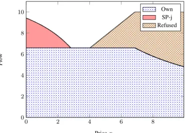
0 2 4 6 8 0 2 4 6 8 10 Pricepj Flo w Own SP-k Refused
Fig. 5. Flow served by providerj, for pk= 4. “Own” denotes the part of
original flowρjserved by providerj, “SP-k” the part from users who agreed
to paypkbut were unserved byk due to capacity constraints, and “Refused”
the part from users who refused to paypk
0 2 4 6 8 0 2 4 6 8 10 Pricepj Flo w Own SP-j Refused
Fig. 6. Flow served by providerk for pk= 4. “Own” denotes the part of
the original flowρkserved by providerk, “SP-j” the part from users agreeing
to paypjbut unserved byj due to capacity constraints, and “Refused” is the
part of users refusing to paypj.
Without loss of generality we consider that⇢1= ↵⇢2= ↵⇢,
for ↵ 2 (0, 1]. (The case ↵ = 0 is trivial and not considered here.) In all this subsection, we consider a linear willingness-to-pay function, i.e.,w(p) = 1 − p/pmax for somepmax> 0.
We consider two cases separately:
1) Whenp1 p2, the provider revenue functions are
(
R1= p1(w(p1)⇢(1 + ↵) − w(p2)⇢),
R2= p2w(p2)⇢.
After getting derivatives and equating them to zero, we get the following pair of prices, as a Nash equilibrium
candidate: ( ¯ p1=pmax2(1+↵)(↵+1/2), ¯ p2=pmax2 .
Note thatp¯2> ¯p1for all ↵ 2 (0, 1]. As can be checked
(see Appendix A in [7]), this pair of prices is indeed a Nash equilibrium for all↵ 2 (0, 1].
The corresponding total revenue is R = R1+ R2=
pmax⇢(↵2+ 2↵ + 5/4)
4(1 + ↵) .
2) When p1> p2, the revenue functions are:
(
R1= p1w(p1)↵⇢,
R2= p2(w(p2)⇢(1 + ↵) − w(p1)↵⇢),
giving the NE candidate (
¯
p1= pmax2 ,
¯
p2= pmax2(1+↵)(1+1/2↵).
Again, for all↵ 2 (0, 1], ¯p1 > ¯p2 is verified. But this
pair of prices is a Nash equilibrium only for↵ 2 [s, 1], wheres ⇡ 0.73 (the details are provided in Appendix A of [7]). The corresponding total revenue is
R = pmax⇢(5/4↵
2+ 2↵ + 1)
4(1 + ↵) .
Summarizing, with large capacities the pricing game has( 1 equilibrium if ↵ 2 (0, s),
2 equilibria if ↵ 2 [s, 1], with s ⇡ 0.73.
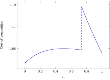
We now compare the minimum total revenue in the duopoly case with the revenue a monopolist would obtain, to evaluate the cost of competition. Following the literature on the Price of Anarchy [11], we use the ratio between the total revenue in the worst-case Nash equilibrium and the monopoly total revenue as the cost measure.
It is easy to check, that the second Nash equilibria high-lighted before –corresponding to the case p1 > p2– gives a
lower total revenue if it exists. Our cost of competition, as a function of ↵, therefore has two segments:
( 4(1+↵3 ) (3+4↵)(↵2+2↵+5/4) if↵ 2 (0, s), 4(1+↵3 ) (3+4↵)(5/4↵2+2↵+1) if↵ 2 [s, 1]. (11) Remark that if we consider only the best-case Nash equilib-rium (under a Price of Stability logic), then the first expression above applies for ↵ 2 [0, 1]. Figure 8 shows the cost of competition of (11), that is maximum for ↵ = s, i.e., when the second candidate becomes actually an equilibrium. For computation details see Appendix B in [7].
B. Homogeneous flows and arbitrary capacities
With arbitrary capacities, the model becomes intractable analytically. We treat here the special case when user flows are homogeneous, i.e., ⇢1 = ⇢2:= ⇢. In that case, we can prove
necessary conditions for a price profile to be an equilibrium.
Proposition 3: If (¯pj, ¯pk) is an equilibrium, then
¯
pj> pcj(¯pk),
¯
Proof:We first prove that if at least one provider –sayj– charges a price lower than or equal to his capacity saturation price, then the price profile is not an equilibrium. Assume that (¯pj, ¯pk) is an equilibrium, with ¯pj < pcj(¯pk): then provider j is
saturated and gets revenuep¯jc. But deviating to pcj(¯pk) would
improve his revenue toRj = pcj(¯pk)c, a contradiction.
Now we prove that there is no equilibrium where at least one provider charges his exact capacity saturation price. Again we assume that(¯pj, pck(¯pj)) is an equilibrium. From the result
above we necessarily have p¯j ≥ pcj(pck(¯pj)), hence ⇢spj = 0.
• We first show that ¯pj ≥ pck(¯pj): if it were not the case
(¯pj < pck, omitting writing p¯j in the saturation price of k)
thenw(¯pj) ≥ w(pck(¯pj)), yielding
⇢T
k(¯pj, pck) = w(pck)⇢ = c,
⇢T
j(¯pj, pck) = 2w(¯pj)⇢ − w(pck)⇢ = 2w(¯pj)⇢ − c c.
This implies w(¯pj) w(pck), therefore w(¯pj) = w(pck)
thus ⇢T
j(¯pj, pck) = c, yielding ¯pj pcj(pck(¯pj)). Since the
opposite inequality also holds we have p¯j = pcj(pck(¯pj)), i.e.,
each provider charges his saturation price. We then deduce that they are equal, because they are both maximum prices such that w(p)⇢ = c, which contradicts our assumption that ¯
pj < pck(¯pj).
• Therefore ¯pj ≥ pck(¯pj). Consider some p > ¯pj; we have
Rj(p, pck(¯pj)) = pw(¯pj)⇢ ⇣ 2 − c 2w(pc k)⇢ − w(¯pj)⇢ ⌘ . We now prove that this revenue, as a function of p, has a positive right-derivative atp = ¯pj. Differentiating, we get
R0 j(p, p c k(¯pj)) = (pw0(p)⇢ + w(p)⇢) ⇣ 2 − c 2w(pc k)⇢ − w(p)⇢ ⌘ −pw(p)⇢ cw 0(p)⇢ (2w(pc k)⇢ − w(p)⇢)2 . At(¯pj, pck(¯pj)) the flow of provider k equals c:
⇢T k(¯pj, pck(¯pj)) = w(pck)⇢ + (w(pck)⇢ − w(¯pj))⇢) = c, which implies R0 j(¯pj, pck(¯pj)) = w(¯pj)⇢ + ⇢¯pjw0(¯pj)(1 − w(¯pj)⇢/c). (12) If w0(¯p
j) = 0, R0j(¯pj, pck(¯pj)) is strictly positive. We now
show it is also the case ifw0(¯p j) < 0. • First, ifp¯j > pcj(pck(¯pj)), then
R0
j(¯pj, pck(¯pj)) = w(¯pj)⇢ + ⇢¯pjw0(¯pj)(1 − w(¯pj)⇢/c)
> w(¯pj)⇢ + ⇢¯pjw0(¯pj).
But as an equilibrium price, p¯j should maximize the
revenue of providerj over (pc
j(pck(¯pj)), pmax), and thus
¯
pj should make the derivative of Rj = pw(p)⇢ equal
to zero, giving w(¯pj)⇢ + ⇢¯pjw0(¯pj) = 0, which implies
R0
j(¯pj, pck(¯pj)) > 0 . • Second, ifp¯j= pc
k(¯pj), then w(¯pj)⇢ = c and the revenue
function derivative in (12) is equal toc > 0.
Thus by increasing his price Provider j could increase his revenue, therefore(¯pj, pck(¯pj)) is not an equilibrium.
Formally, in order to show that a pair of prices is an equilibrium, we have to compare the revenue they yield with the maximum revenues in all other zones (as defined in Subsection IV-B) for each provider. Proposition 3 reduces this search, to zones where both prices are strictly above capacity saturation prices. It can be easily checked that situations where providers charge equal prices cannot be equilibria. Therefore the equilibrium candidates remaining can be characterized by
8 > < > : p16= p2, p1> pc1(p2); p2> pc2(p1), R0 1(p1, p2) = 0; R02(p1, p2) = 0,
To show that such pairs are indeed Nash equilibria, we have to compare the revenue they give with the maximum revenue in other segments.
For a linear willingness-to-pay function, the system above only leaves two candidates
(¯p1, ¯p2) 2 {(1/2pmax, 3/8pmax), (3/8pmax, 1/2pmax)} (13)
Numerically, we found that these two pairs of prices are indeed equilibria only when ⇢/c t, with t ⇡ 1.23. Figure 7 shows the best-response curves when ⇢/c = t.
C. The cost of ignoring competition
In our scenario, providers may not be aware of the presence of each other (especially if they are located far from each other), and thus do not play a noncooperative game on prices. In that case each provider would treat users seeing him first the same way as he treats those coming from the competitor’s direction. We estimate here the cost of this ignorance in terms of revenue loss.
Then each providerj would believe his total flow to be ⇢1+
⇢2 independently ofpj, and would therefore simply select his
price so as to maximizepjmin(c, (⇢1+⇢2)w(pj)), leading to a
situation wherep1= p2= arg maxpp min(c, (⇢1+ ⇢2)w(p)).
But from that situation, one provider could decrease his price and also serve users from the competitor who found him too expensive. For a linear willingness-to-pay function, we found that in the symmetric-flow case, this price shift would yield a 12.5% revenue increase, and in the large capacity case with heterogeneous flows, an approximate 33% revenue increase for ↵ = 1/2 (see Appendix C in [7]).
VI. CONCLUDINGREMARKS
In this work, we have analyzed the price competition between roadside units operators which are providing wireless access to moving vehicles. In contrast to general work on pricing in wireless networks where wireless operators compete on price to attract “common” users, in the reference scenario competition arises due to vehicles mobility even if the roadside units do not have overlapped coverage areas. The strategic interaction between two roadside units operators is analyzed through game theoretic tools. Namely, the analysis of the best-response function having fixed the competitor’s price
0 2 4 6 8 10 0 2 4 6 8 10 Pricep1 Price p2 p1=BR1(p2) p2=BR2(p1)
Fig. 7. Best-response curves in the general case, whenpmax= 10, for the
maximum value ofρ/c such that an equilibrium exists. At the equilibrium
point (3.75, 5), the best-response function of Provider 2 is discontinuous: that provider is indifferent between the maximum in the segment where Provider 1 is saturated (⇡ 6.2) and the maximum in the segment where provider 1 is not saturated (3.75). 0 0.2 0.4 0.6 0.8 1 1.08 1.1 1.12 α Cost of competition
Fig. 8. Cost of competition for large capacities in the heterogeneous-flows
case (α small corresponds to high flow heterogeneity). The cost of competition function is discontinuous (because the least efficient equilibrium does not exist
for allα) and reaches its maximum at α = s.
sheds light on interesting and counterintuitive behaviors in the systems which lead one roadside unit operator to increase her price to induce higher interference onto the competitor, thus causing traffic spillover from the competitor’s side. The results from the best-response analysis are then leveraged to characterize the simultaneous competitive game between the two roadside units operators in terms of equilibrium existence and optimality. A natural follow-up for the present work includes the analysis of the scenario in which the strategy space of each roadside unit operator also includes the position of the roadside unit besides setting the price.
REFERENCES
[1] E. Altman, A. Kumar, C. Singh, and R. Sundaresan, “Spatial SINR games combining base station placement and mobile association,” in
Proc. of IEEE INFOCOM, 2009.
[2] J. Barrachina, P. Garrido, M. Fogue, F. Martinez, J.-C. Cano, C. Calafate, and P. Manzoni, “Road side unit deployment: A density-based ap-proach,” IEEE Intelligent Transportation Systems Magazine, vol. 5, no. 3, pp. 30–39, 2013.
[3] C. Berge, Topological spaces. Dover Publications, 1963.
[4] F. Borgonovo, A. Capone, M. Cesana, and L. Fratta, “ADHOC MAC: New MAC architecture for ad hoc networks providing efficient and reliable point-to-point and broadcast services,” Wirel. Netw., vol. 10, no. 4, pp. 359–366, Jul. 2004.
[5] E. S. Cavalcante, A. L. Aquino, G. L. Pappa, and A. A. Loureiro, “Roadside unit deployment for information dissemination in a VANET: An evolutionary approach,” in Proc. of GECCO Companion, 2012. [6] I. Filippini, F. Malandrino, G. Dan, M. Cesana, C. Casetti, and I. Marsh,
“Non-cooperative RSU deployment in vehicular networks,” in Proc. of
WONS, 2012.
[7] V. Fux, P. Maill´e, and M. Cesana, “Price competition between road side units operators in vehicular networks,” 2014. [Online]. Available: http://hal.archives-ouvertes.fr/hal-00967110
[8] V. Fux and P. Maill´e, “Incentivizing efficient load repartition in hetero-geneous wireless networks with selfish delay-sensitive users,” in Proc.
of ICQT, 2013.
[9] H. Hartenstein and K. Laberteaux, “A tutorial survey on vehicular ad hoc networks,” Communications Magazine, IEEE, vol. 46, no. 6, pp. 164–171, 2008.
[10] S. Kakutani, “A generalization of Brouwer’s fixed point theorem,” Duke
Mathematical Journal, vol. 8, pp. 457–459, 1941.
[11] E. Koutsoupias and C. Papadimitriou, “Worst-case equilibria,” in
Pro-ceedings of the 16th annual conference on Theoretical aspects of
computer science, 1999.
[12] U. Lee, E. Magistretti, M. Gerla, P. Bellavista, and A. Corradi, “Dissem-ination and harvesting of urban data using vehicular sensing platforms,”
IEEE Transactions on Vehicular Technology, vol. 58, no. 2, pp. 882–901,
2009.
[13] P. Maill´e and B. Tuffin, Telecommunication Network Economics: From
Theory to Applications. Cambridge University Press, 2014.
[14] D. Niyato and E. Hossain, “Competitive pricing in heterogeneous wire-less access networks: Issues and approaches,” IEEE Network, vol. 22, no. 6, 2008.
[15] ——, “A unified framework for optimal wireless access for data stream-ing over vehicle-to-roadside communications,” IEEE Transactions on
Vehicular Technology, vol. 59, no. 6, pp. 3025–3035, 2010.
[16] D. Niyato, E. Hossain, and P. Wang, “Competitive wireless access for data streaming over vehicle-to-roadside communications,” in Proc. of
IEEE GLOBECOM, 2009, pp. 1–6.
[17] D. Niyato, E. Hossain, and M. Hassan, Game-Theoretic Models
for Vehicular Networks. CRC Press, 2011. [Online]. Available:
http://dx.doi.org/10.1201/b10975-6
[18] M. J. Osborne and A. Rubinstein, A Course in Game Theory.
Cam-bridge, 1994.
[19] W. Saad, Z. Han, A. Hjorungnes, D. Niyato, and E. Hossain, “Coalition formation games for distributed cooperation among roadside units in vehicular networks,” IEEE JSAC, vol. 29, no. 1, pp. 48–60, Jan. 2011. [20] O. Trullols, M. Fiore, C. Casetti, C. Chiasserini, and J. B. Ordinas, “Planning roadside infrastructure for information dissemination in in-telligent transportation systems,” Computer Communications, vol. 33, no. 4, pp. 432 – 442, 2010.
[21] T. Yan, W. Zhang, G. Wang, and Y. Zhang, “Access points planning in urban area for data dissemination to drivers,” IEEE Transactions on
Vehicular Technology, 2013.
[22] K. Yang, S. Ou, H.-H. Chen, and J. He, “A multihop peer-communication protocol with fairness guarantee for IEEE 802.16-based vehicular net-works,” IEEE Transactions on Vehicular Technology, vol. 56, no. 6, pp. 3358–3370, 2007.
[23] X. Yang, J. Liu, N. Vaidya, and F. Zhao, “A vehicle-to-vehicle com-munication protocol for cooperative collision warning,” in Proc. of
MOBIQUITOUS, 2004, pp. 114–123.
[24] Y. Zhang, J. Zhao, and G. Cao, “On scheduling vehicle-roadside data
access,” in Proc. of ACM VANET. New York, NY, USA: ACM, 2007,