HAL Id: hal-01128761
https://hal-mines-paristech.archives-ouvertes.fr/hal-01128761
Submitted on 10 Mar 2015
HAL is a multi-disciplinary open access
archive for the deposit and dissemination of
sci-entific research documents, whether they are
pub-lished or not. The documents may come from
teaching and research institutions in France or
abroad, or from public or private research centers.
L’archive ouverte pluridisciplinaire HAL, est
destinée au dépôt et à la diffusion de documents
scientifiques de niveau recherche, publiés ou non,
émanant des établissements d’enseignement et de
recherche français ou étrangers, des laboratoires
publics ou privés.
Copyright
A model to take advantage of Physical Internet for
vendor inventory management
Yanyan Yang, Shenle Pan, Eric Ballot
To cite this version:
Yanyan Yang, Shenle Pan, Eric Ballot. A model to take advantage of Physical Internet for vendor
inventory management. 2015 IFAC Symposium on Information Control in Manufacturing (INCOM
2015), May 2015, Ottawa, Canada. �hal-01128761�
*MINES ParisTech, PSL Research University, CGS - Centre de Gestion Scientifique 60 Bd Saint-Michel, 75272 Paris Cedex 06, France
(Tel: +33- 140519197; e-mail: {yanyan.yang; shenle.pan; eric.ballot}@mines-paristech.fr).
Abstract: This paper investigates inventory management problems for fast-moving consumer goods (FMCG) with the Physical Internet (interconnected logistic services) where goods are stored and distributed in an interconnected and open network of hubs. Unlike current hierarchical inventory model where the source assignment is predetermined for each replenishment order either from the retailers or from the warehouses, the PI-inventory model enables multiple source selection options to each order and transshipments of inventories among hubs, resulting in complete pooling of inventories within the network. We adopt a continuous review (Q, R) ordering policy for each facility and propose four dynamic source selection strategies related to the supplying nodes’ inventory levels, the distance and lead time between the supplying and the ordering nodes. The objective is to determine the optimal replenishment policies for hubs in order to minimize the total logistic costs of the distribution system. A nonlinear optimization model is proposed and a heuristic using simulated annealing is applied. A simulation study based on two categories of FMCG is taken to evaluate the performance of the proposed inventory control policies. Our results suggest that compared to current centralized inventory control policy, the PI-inventory control model with proposed source selection strategies can significantly reduce the total costs as well as the average inventory level of the network of hubs while reaching the same end customer service level.
Keywords: Inventory control, Physical Internet, dynamic source selection, multiple sourcing, FMCG
1. INTRODUCTION
In the past decades, a great number of papers have dealt with inventory problems based on centralized or hierarchical inventory systems as inventory often accounts for a large proportion of a company’s supply chain management costs. In this paper, we study inventory problems in the recently proposed open and interconnected logistic network called Physical Internet. Inspired by the metaphor of Digital Internet, the Physical Internet (PI) aims to integrate logistics networks into an open and interconnected global system through standard containers and routing protocols (Ballot and Montreuil, 2014). Concerning inventory problems, unlike classical storage organization in actual logistic systems, the PI network enables a distributed storage of goods in hubs which may be managed by the Logistic Service Providers (LSP) and shared by companies including suppliers and their customers (retailers). The replenishment orders either from the hubs or from the retailers are no longer pre-assigned to specific supplying points and are dynamically decided according to different source selection strategies. Theoretically, each supplier can store their goods at any hub all around the network and each hub or customer can be served by any other hubs or directly by the supplier, which makes it feasible for the sharing of inventories and transportation, and also the multiple source options for replenishment orders. This system enables more supply strategies that will be used when needed. Thus, this kind of inventory management structure would potentially lead to lower inventory levels and improved customer service levels, resulting lower total cost. Under this structure, our research questions lie on: 1) how to respond to each
replenishment order with required constraints; 2) how to determine inventory replenishment policies for hubs under these source selection strategies.
Following the previous works studying inventory problems in Physical Internet, we can conclude three main characteristics of the inventory problems in the Physical Internet: 1) dynamic source selection; 2) multiple source selection options to one order; 3) transshipments of inventories among hubs. Therefore, in this paper, we investigate the inventory control models corresponding to these three main characteristics and analyse how they affect the whole supply chain. Our objective is to provide optimal replenishment policies for each hub under different source selection strategies and to compare the overall supply chain performance of our inventory control policies to the current inventory control policy with predetermined mono source selection strategy. The policies and the models proposed here can be further implanted as a decision-making tool.
To gain insight into this question, we study a single FMCG (fast moving consumer good) product inventory problem in a Physical Internet network of hubs supplying a group of retailers which face normal distributed end-customer demands. We adopt a centralized vendor-decision framework for the supplier who determines the inventory control policies for the warehouses or the hubs. The objective is to determine optimal inventory control policies for hubs to minimize the total cost of the distribution system while satisfying replenishment orders from retailers. We suppose the optimal replenishment parameters at retailers are obtained to minimize its own total cost under the assumption of infinite inventory
supplier. Four dynamic source selection strategies related to the inventory levels of the supplying points, the distance and lead time between the supplying and ordering points are proposed. A nonlinear optimization model is described and a heuristic using simulated annealing is applied. Policies are evaluated by simulation studies. Our results suggests that the PI-inventory model with dynamic source selection strategies can significantly reduce the supply chain management cost compared to current centralized predetermined inventory control strategy while reaching the same end customer service level at retailers (defined as the percentage of customer satisfied by inventory on hand).
Within the literature we found the following two inventory control models based on current hierarchical inventory system close to the PI inventory modality: i) inventory models with lateral transshipments that allow inventory movements among members of the same echelon; ii) inventory models with multi-sourcing options which enables a replenishment order to be satisfied by multiple supplying points. Recent comprehensive overview about lateral transshipment is provided by (Paterson et al., 2011). Two types of transshipments are often addressed according to the timing of the transshipments: 1) reactive transshipments in response to an existing stock-out as seen in (Krishnan and Rao, 1965), (Robinson, 1990), (Olsson, 2010); 2) proactive transshipments to prevent the future stock-out, as seen in (Gross, 1963), (Diks and De Kok, 1998), (Tagaras and Vlachos, 2002). The literature has shown that transshipment is quite profitable for retailers with long replenishment lead times from suppliers and who are located closer to one another or who have grand shortage penalty cost. In spite of the horizontal sharing of inventories in both transshipments and PI inventory model, the hubs in the Physical Internet are fully interconnected and the source selection is dynamically determined while in the lateral transshipments the source is pre-assigned and the transshipments are used as a support to regular replenishment orders.
The research of the multi-sourcing inventory model can be divided into two categories according to whether an order can be split into sub-quantities and met by several source supplying points: 1) without order splitting which focus on source substitution method, as seen in (Ng et al., 2001), (Çapar et al., 2011), (Veeraraghavan and Scheller-Wolf, 2008); 2) with order splitting which focus on inventory allocation method in addition to source substitution, as seen in (Sculli and Wu, 1981), (Ryu and Lee, 2003), (Song et al., 2014). The literature shows that the multi-sourcing can reduce the mean and variance of the effective lead time and a split order model always has lower stock levels than the equivalent non-split model. However, the sourcing options in current multi-sourcing models are only restricted between the upper level stocking points and their successive demanding points. The same echelon stocking points are independent and no products flow at the same echelon stocking points are allowed. Therefore we conclude that our model differs from inventory models existing in literature.
The rest of this paper is organized as follows: Section 2 presents details of the problem description and assumptions; Section 3 propose a non-linear optimization formulation and solution approach; Section 4 presents and analyses the
numerical results. Finally, Section 5 gives conclusions and remarks for the further research.
2. PROBLEM DESCRIPTION AND ASSUMPTIONS
2.1 The PI replenishment schemes
To simplify the problem without losing the generality, here we consider a single product PI-inventory system under continuous review with a plant (indexed by 0) supplying a network of M hubs (indexed by i) and Nr retailers/markets (indexed by j) which face independent normal distribution end customer demand, i.e. an example of three hubs and four retailers depicted in (Fig. 1. b). (Fig. 1. a) shows the corresponding replenishment scheme for classical centralized inventory model where a warehouse supplying two distribution centers belong to two different retailer companies with two points of sales. Localizations remain the same in all scenarios.
Fig. 1. Centralized inventory model VS PI inventory model As seen in (Fig. 1. a), under the classical inventory models, the product flow directions are predetermined. Each points of sales are pre-assigned to their own distribution center, i.e. R1 and R2 can only be supplied by DC1. The DCs’ replenishment order can only be met by the warehouse and no transhipments among DCs and direct shipments from the plant to the DCs under this inventory control policy are allowed. For example, under this hierarchical structure, if DC1 faces a stock-out, the replenishment orders from points of sales R1 and R2 cannot be satisfied even if the DC2 and the warehouse have high inventory levels. However, in the PI-inventory control model depicted in (Fig. 1. b), there exist no more echelons and the network of hubs are fully open and interconnected. The hub center coordinates the movement of stocks around the network to meet replenishment orders from points of sales. In detail, the replenishment orders from any of the points of sales can be served by any hub around the network and the hubs can be supplied by any other hub or the plant. Therefore, if the hub2 faces a stock-out, the replenishment orders from points of sales R1 or R2 can either be met by hub1 or hub3 under required
constraints by different source selection options, resulting in reduced lead times and reduced lost sales. Besides, the interconnected network also facilitate the mutualisation of transportation flows, resulting in reduced transportation cost and reduced total inventory level around the network by augmenting the transportation frequency between the plants and the distribution network. Based on the above analysis, we can see that the inventory decisions for this PI-inventory model concern to two parts: 1) source selection strategy for each replenishment order; 2) inventory control policies for hubs.
2.2 PI inventory control model
In this paper, four dynamic source selection options are proposed: 1) S1 - Minimum distance: among the supplying points with inventory level bigger than the ordering quantity, choose the nearest candidate to the ordering point; 2) S2 - Maximum stock on hand: among the supplying points with inventory level bigger than the ordering quantity, choose the candidate with the highest inventory level; 3) S3 - Maximum ratio of (inventory level/lead time): among the supplying points with inventory level bigger than the ordering quantity, choose the candidate with the maximum ratio of (inventory level/lead time between the candidate and the ordering point); 4) S4 - Maximum ratio of (inventory level/distance): among the supplying points with inventory level bigger than the ordering quantity, choose the candidate with the maximum ratio of (inventory level/distance between the candidate and the ordering point). The scenario of current pre-determined source selection method is also studied and indexed by S0. For the five scenarios, we adapt the following common assumptions: a) Each stocking facility including hubs and retailers applies a (R, Q) continuous review policy; b) The plant is assumed to always have adequate stocks to meet the demands and there is no capacity constraint for hubs; c) Unmet replenishment orders from retailers are considered with a penalty cost that is assumed to be proportional to the retailer’s average daily demand quantity and the product value; d) The lead times among all the interconnected facilities are given and assumed to be constant; e) The orders are served on a first-come-first-served basis; f) No partial delivery is allowed; g) End customer demands to retailers are uncertain and subject to normal distribution; h) Vendor makes all source selections to supply the retailers.
Within the economic scale, four logistic costs are considered: inventory holding cost, transportation cost, ordering cost and the penalty cost for unmet demands. The holding cost are charged for each unit in stock per time unit both at retailers and hubs. The transportation cost for each delivery of goods are considered and is a proportional function of the distance and quantity travelled. Besides, each replenishment order placed incurs a fixed ordering cost. Penalty cost for unsatisfied order from retailers and lost sales for unmet customer demands at retailers are considered and are proportional to the product value and unmet quantity.
We adopt a centralized vendor-decision framework for the hub system who distributes goods around the network of hubs, in order to meet the demands from the retailers where the inventory decisions are made by their own manager to
minimize its total cost of the same categories with required lead time constraints. In this paper, the optimal replenishment parameters (𝑞𝑗∗, 𝑠𝑗∗) for each retailer j are determined by the
algorithm proposed by (Giard, 2005). The optimal replenishment parameters (𝑞𝑗∗, 𝑠𝑗∗) for each retailer j are considered as input information for the hub system under all scenarios. With optimal replenishment policies and normal distributed daily demand, when the inventory position at retailer j drops below the reorder point 𝑠𝑗∗, it places an
replenishment order with quantity 𝑞𝑗∗ at the hub system. The
hub system choose among the candidate hubs to respond the demand according to different dynamic source selection strategies. The objective is determine the optimal replenishment parameters of hubs under different source selection methods to minimize the total cost including holding cost at hubs, transportation cost to satisfy the replenishment orders both from hubs and the retailers, penalty cost for unmet orders from retailers, and the fixed ordering cost for each replenishment order placed by hubs.
3. FORMULATION AND SOLUTION APPROACH
3.1 Formulation
We adapt a discrete event modelling method. To introduce the optimization model, we use the following notations. And we always refer to SKU to the minimum unit we consider in the model.
𝑀: set of hubs (plant index by 0). 𝑁𝑟: set of retailers.
𝑇: configuration time the inventory system, indexed by 𝑛 (1 year = 365 days).
𝑑𝑖𝑠𝑖𝑗: distance between hub 𝑖 ∈ 𝑀 and retailer 𝑗 ∈ 𝑁𝑟.
𝑑𝑖𝑠𝑘𝑖: distance between hub 𝑘 ∈ 𝑀 and hub 𝑖 ∈ 𝑀 .
𝑑𝑖𝑠0𝑖 : distance between hub 𝑖 ∈ 𝑀 and the plant 0.
(𝑢𝑗, 𝜎𝑗) : average and standard deviation of end customer
demand at retailer 𝑗.
(𝑞𝑗, 𝑠𝑗): replenishment policy of retailer 𝑗 - 𝑞𝑗 for batch size
and 𝑠𝑗 for reorder point.
𝐻𝑖: daily holding cost per SKU at hub 𝑖.
𝑐1: transportation cost per kilometer per SKU from the hubs to
retailer - computed by the cost for a full truckload divided by the number of SKU per full truckload.
𝑐2: transportation cost per kilometer per SKU from the plant to
hubs and among hubs - the same calculation as 𝑐1.
𝑝𝑗: daily penalty cost per SKU of unmet orders from retailer
𝑗 ∈ 𝑁𝑟.
𝐴: the fixed ordering cost per order.
𝐼𝐿𝑖𝑛/𝐼𝐿𝑗𝑛: inventory level at hub 𝑖 / retailer 𝑗 between 𝑛th and
(𝑛 + 1)th day.
𝐼𝑃𝑖𝑛/𝐼𝑃𝑗𝑛: inventory position at hub 𝑖 / retailer 𝑗 between 𝑛th
The parameters of the five scenarios are optimized. The decision variables are:
𝑅𝑖: hub 𝑖’s reorder point.
𝑄𝑖0: hub 𝑖’s batch size (order quantity) from the plant.
𝑄𝑖: hub 𝑖’s batch size (order quantity) from other hubs.
𝑥0𝑖𝑛: binary variable of whether choose plant 0 to satisfy the
demand of hub 𝑖 at time 𝑛th day, if so 𝑥0𝑖𝑛 = 1, otherwise 0;
𝑥𝑘𝑖𝑛: binary variable of whether choose hub 𝑘 ∈ 𝑀 to satisfy
the demand of hub 𝑖 (𝑖 ≠ 𝑘) at time 𝑛th day.
𝑥𝑘𝑗𝑛: binary variable of whether choose facility 𝑘 ∈ 𝑀 to
satisfy the demand of retailer 𝑗 at time 𝑛th day. The objective function:
𝑀𝑖𝑛𝑖𝑚𝑖𝑧𝑒 𝐶𝑡𝑜𝑡 = [∑ ∑ 𝐼𝐿𝑖𝑛𝐻𝑖 𝑇 𝑛=1 𝑀 𝑖=1 ] (1) + [∑ ∑ ∑ 𝑥𝑘𝑗𝑛𝑐1 𝑀 𝑘=1 𝑇 𝑛=1 𝑁𝑟 𝑗=1 𝑞𝑗𝑑𝑖𝑠𝑘𝑗] (2) + [∑ ∑ ∑ 𝑥𝑘𝑖𝑛(𝑐2𝑄𝑖𝑑𝑖𝑠𝑘𝑖+ 𝐴) 𝑀 𝑘=1,𝑘≠𝑖 𝑇 𝑛=1 𝑀 𝑖=1 ] (3) + [∑ ∑ 𝑥0𝑖𝑛(𝑐2𝑄𝑖0𝑑𝑖𝑠0𝑖+ 𝐴) 𝑇 𝑛=1 𝑀 𝑖=1 ] (4) + [∑ ∑ (1 − ∑ 𝑥𝑘𝑗𝑛 𝑀 𝑘=1 ) ∗ 𝑞𝑗 𝑁𝑟 𝑗=1 ∗ 𝑝𝑗 𝑇 𝑛=1 ] (5) Subject to: 0 ≤ ∑𝑀𝑘=1𝑥𝑘𝑗𝑛≤ 1 ∀𝑗 ∈ 𝑁𝑟, ∀𝑛 = 1 … 𝑇 (6) 𝑥𝑘𝑗𝑛∈ {0,1}, ∀𝑘 ∈ 𝑀, ∀𝑗 ∈ 𝑁𝑟, ∀𝑛 = 1 … 𝑇 (7) 0 ≤ ∑𝑀𝑘=0,𝑘≠𝑖𝑥𝑘𝑖𝑛≤ 1 ∀𝑖 ∈ 𝑀, ∀𝑛 = 1 … 𝑇 (8) 𝑥𝑘𝑖𝑛∈ {0,1}, ∀𝑖 ∈ 𝑀, ∀𝑘 ∈ 𝑀 ∪ {0}, 𝑖 ≠ 𝑘, ∀𝑛 = 1 … 𝑇 (9) 𝑅𝑖, 𝑄𝑖0, 𝑄𝑖:Integers, ∀𝑖 ∈ 𝑀 (10)
Where (1) represents the total annual holding cost at the hubs, (2) indicates the total annual transportation cost to satisfy replenishment orders from retailers, (3) describes the total annual transportation cost and fixed ordering cost to meet the replenishment orders of the hubs by other hubs, (4) presents the total annual transportation cost and fixed ordering cost to meet the replenishment orders of the hubs by the plant, (5) introduces the penalty cost for unmet replenishment orders from the hubs. Constraints (6) - (9) describe that the replenishment orders can only be met by one facility each time. Hence, order splitting is not allowed in the model. Constraint (10) indicates that the demanding quantity cannot be allowed fractional or partial.
3.2 Solution approaches
To solve the nonlinear global optimization problem, we use the source selection strategies to determine the source selection variables 𝑥0𝑖𝑛/𝑥𝑘𝑖𝑛/𝑥𝑘𝑗𝑛 and a simulated annealing algorithm
adapted to further optimize the replenishment parameters for hubs under each sourcing strategy. The following procedure calculates the annual total cost for each replenishment parameters of hubs (𝑄𝑖0, 𝑄𝑖, 𝑅𝑖) in the heuristic algorithm.
Simulation-based annual total cost calculation procedure:
Input: (𝑄𝑖0, 𝑄𝑖, 𝑅𝑖) and – the optimization computed by the
simulated annealing algorithm.
Step 1: Initialize 𝑛 = 1 (time), initial stock at every hubs to be 0 SKU and (𝑠𝑗+ 𝑞𝑗) for each retailer j.
Step 2: Randomly generate end customer demands according to normal distribution function respecting input parameters (𝑢𝑗, 𝜎𝑗) at retailer 𝑗 ∈ 𝑁𝑟 , update inventory level 𝐼𝐿𝑗𝑛 and
inventory position 𝐼𝑃𝑗𝑛, unmet end customers demands are considered as lost sales.
Step 3: For each retailer j, if inventory position 𝐼𝑃𝑗𝑛≤
𝑠𝑗, based on source selection strategy, determine the source 𝑖∗
( 𝑥𝑖∗𝑗𝑛= 1), update the inventory information of retailer j and
the source 𝑖∗.
Step 4: For each hub i, if inventory position 𝐼𝑃𝑖𝑛 ≤ 𝑅𝑖, based
on source selection strategy, determine the source 𝑘∗ ( 𝑥 𝑘∗𝑖𝑛=
1), update the inventory information of hub i and the source 𝑘∗.
Step 5: If 𝑛 ≤ 𝑇, 𝑛 + + and go to Step 2.
Step 6: Calculate and return annual total cost 𝐶𝑡𝑜𝑡.
4. NUMERICAL RESULTS
This section reports the results from a simulation study that evaluates logistic costs with the optimal replenishment parameters for the five source selection strategies obtained by a simulated annealing heuristic method.
Two cases studies have been taken: an example of mineral water where the transportation cost is much bigger than the holding cost and lost sales, and an example of washing products where the products value are 5 times more expensive than mineral water resulting in holding cost and lost sales more expensive. We test on a single product PI-inventory system with three hubs and four retailers. Daily demands at retailers are assumed to be same for all the experiments which follows normal distribution function (u, σ):(5, 3), (6, 3), (3, 1), (4, 2) expressed in SKU. The fixed ordering cost for each order is assumed to be 𝐴 = 20 (monetary unit) per order (or 0 if the order is not satisfied). The penalty cost for unmet orders from retailers to hubs is considered as 20% of the product value while it is 30% for the lost sales at retailers. The transportation cost from the plant to hubs and among hubs is assumed to be 1.4 per full truckload per kilometer and 2.0 per full truckload per kilometer from hubs to retailers. This assumption is based on the fact that the transportation cost for long-haul full truck-load is lower than that the last mile transportation cost. The lead time are assumed to be 5 days between the plant and hubs, 1 day between hubs and 2 days between hubs and retailers.
Table 1 presents the distance matrix of the network. With all these setups and the methods presented in (Giard, 2005), we can therefore obtain the optimal replenishment parameters (𝑞𝑗∗, 𝑠𝑗∗) for retailers, as depicted in Table 2.
Table 1. Distance (km) Plant H1 H2 H3 H1 200 0 160 155 H2 350 160 0 165 H3 325 155 165 0 R1 170 15 160 R2 140 165 15 R3 100 95 90 R4 90 100 105
Table 2. Optimal policies for retailers (𝒒𝒋∗, 𝒔𝒋∗) (SKUs)
Case Nodes Case 1 (product value =24 /SKU) Case 2 (product value = 120 /SKU) R1 (85, 16) (65,19) R2 (93, 19) (71, 21) R3 (65, 8) (50, 9) R4 (76, 12) (58, 14) From Table 2, we can see that the reorder points for retailers are bigger in Case 2 than in Case 1 since the product value is more expensive which results in more expensive holding cost and lost sales (recall that we assume they have the same demand rate). The optimal replenishment parameters for retailers are considered as input information for the hub system, in order to find the optimal values of (𝑄𝑖0∗, 𝑄𝑖∗, 𝑅𝑖∗) for
each hub i under each source selection strategy. We use a simulated annealing procedure for the optimization. The lower bound for each (𝑄𝑖0, 𝑄𝑖, 𝑅𝑖) is considered as 0 and the upper
bound is chosen as a big quantity (400 SKUs) that can satisfy all the demands from the retailers. All the experimental tests are developed in Mathematica 10.0. The convergence ratio, the maximum temperature and the maximum iteration number are set to be 3%, 60, and 8000.
Table 3 describes the optimal values of (𝑄𝑖0∗, 𝑄𝑖∗, 𝑅𝑖∗) for all the
five sourcing strategies. We can see that in all the instances the optimal value of the reorder point 𝑅𝑖∗ for hub i under dynamic
source selection strategies (S1, S2, S3 et S4) is lower than that under the pre-determined source selection strategy S0. It is a result of inventory sharing among the hubs. And as seen in the table, the lost sizes placed to other hubs under the sourcing strategy S2 are always to be 0. This is explained as the plant is always assumed to have the highest inventory level. Thus under the sourcing strategy 2, the hubs’ replenishment orders are always satisfied by the plant.
Table 3. Optimal policies for hubs
Node
Reorder point
Lot size from plant
Lot size from hubs/warehouse
C
ase1 Case2 Case1 Case2 Case1 Case2
S0 WH 114 138 210 168 DC1 102 78 108 108 DC2 102 90 72 78 S1 H1 78 78 120 144 0 0 H2 84 54 150 138 186 186 H3 78 66 174 132 222 0 S2 H1 108 102 90 150 0 0 H2 72 66 162 96 0 0 H3 90 84 150 90 0 0 S3 H1 108 126 126 108 0 0 H2 72 60 138 180 66 66 H3 72 60 90 132 66 90 S4 H1 102 120 138 114 180 0 H2 90 66 78 66 222 144 H3 96 66 108 138 234 0 With the optimal replenishment parameters for each source selection strategy, we simulated the total system for 100 times and obtain the average total cost of the hub system, the average total level of all hubs, and the average end customer level at retailers, as presented in Table 4 and Table 5. We adapt the performance ratio defined in (Ng et al., 2001) to compare the performance of scenarios. Here we use S0 (current predetermined inventory control strategy) as baseline and the performance ratio to other scenarios is the relative variation in total costs.
Table 4. Simulation results of average cost and performance ratio for Case 1
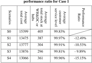
S ce n ar io s Av er ag e to tal co st Av er ag e to tal sto ck at W H& DC o r hubs Aver ag e cu sto m er ser v ice lev el Per fo rm an ce R atio S0 15399 405 99.83% S1 13475 387 99.97% -12.49% S2 13777 304 99.91% -10.53% S3 13876 296 99.81% - 9.89% S4 13066 361 99.96% -15.15%
Table 5. Simulation results of average cost and performance ratio for Case 2
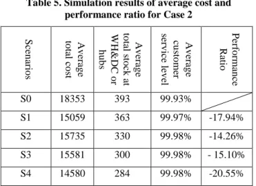
S ce n ar io s Av er ag e to tal co st Av er ag e to tal sto ck at W H& DC o r hubs Aver ag e cu sto m er ser v ice lev el Per fo rm an ce R atio S0 18353 393 99.93% S1 15059 363 99.97% -17.94% S2 15735 330 99.98% -14.26% S3 15581 300 99.98% - 15.10% S4 14580 284 99.98% -20.55% We can see that the average total cost of the hub system can be significantly reduced by the dynamic source selection strategies under the PI-inventory model compared to current pre-determined source selection strategy S0. And the strategy S4 (Maximum ratio of inventory on hand and distance) has the best performance compared to other strategies for both cases. Besides performance ratio increases with the product value, since the inventory holding cost, penalty cost and lost sales are very dependent on the product value. In addition, the average end customer service levels in case 2 are higher than in case 1 due to the higher product value and with the similar customer service level, the average inventory level at the hubs are reduced by the dynamic source selection strategy compared to deterministic sourcing strategy S0.
5. CONCLUSIONS
We have developed and evaluated four dynamic source selection strategies for a PI-inventory model with a plant supplying a network of hubs and retailers. The optimal replenishment policies for hubs are determined for each source selection strategy to minimize the annual total cost of the distribution system including holding cost, fixed ordering cost, transportation cost and penalty cost for unmet orders from retailers. A heuristic using simulated annealing is proposed to solve the optimization problem and then a simulation study is taken to evaluate the optimal policies under each sourcing strategy. The results show all the four dynamic source selection strategies in the PI-inventory model can significantly reduce the average total cost compared to current pre-determined source selection strategy while reaching the same end customer service levels. Besides, the advantage of the dynamic source selection strategies increases when the product value increases.
In this paper, we consider the optimal replenishment policies for retailers as the same as in current inventory models and study how the PI-inventory models affect the inventory control policies for the distribution system. Next step, we will consider the impact of PI-inventory models to the inventory control policies of retailers. Besides, the proposed heuristic algorithm is rather simple and converges slowly considering the problem scale of 9 decisions variables to each problem. Thus, an effort to develop the optimization algorithm with better performance is also an important research topic for the next. Last, only two
types of products have been studied in this paper. More experimentation is necessary to study the impact of PI on various FMCG, inventory control policy, variation in demand, network configuration, etc.
REFERENCES
BALLOT, E. & MONTREUIL, B. (2014). L'internet
physique, le réseau des réseaux des prestations logistiques, 29. Documentation Française, France.
ÇAPAR, İ., EKŞIOĞLU, B. & GEUNES, J. (2011). A decision rule for coordination of inventory and transportation in a two-stage supply chain with alternative supply sources. Computers & Operations Research, 38, 1696-1704.
DIKS, E. & DE KOK, A. (1998). Optimal control of a divergent multi-echelon inventory system. European
Journal of Operational Research, 111, 75-97.
GIARD, V. (2005). Gestion de la production et des flux 3e
Edition, 839. Economica, France
GROSS, D. (1963). Centralized inventory control in multilocation supply systems. Multistage inventory
models and techniques, 1, 47.
KRISHNAN, K. & RAO, V. (1965). Inventory control in N warehouses.
NG, C., LI, L. Y. & CHAKHLEVITCH, K. (2001). Coordinated replenishments with alternative supply sources in two-level supply chains. International Journal
of Production Economics, 73, 227-240.
OLSSON, F. (2010). An inventory model with unidirectional lateral transshipments. European Journal of Operational
Research, 200, 725-732.
PATERSON, C., KIESMÜLLER, G., TEUNTER, R. & GLAZEBROOK, K. (2011). Inventory models with lateral transshipments: A review. European Journal of
Operational Research, 210, 125-136.
ROBINSON, L. W. (1990). Optimal and approximate policies in multiperiod, multilocation inventory models with transshipments. Operations Research, 38, 278-295. RYU, S. W. & LEE, K. K. (2003). A stochastic inventory
model of dual sourced supply chain with lead-time reduction. International Journal of Production Economics, 81–82, 513-524.
SCULLI, D. & WU, S. (1981). Stock control with two suppliers and normal lead times. Journal of the
Operational Research Society, 1003-1009.
SONG, D.P., DONG, J.X. & XU, J. (2014). Integrated inventory management and supplier base reduction in a supply chain with multiple uncertainties. European
Journal of Operational Research, 232, 522-536.
TAGARAS, G. & VLACHOS, D. (2002). EFFECTIVENESS OF STOCK TRANSSHIPMENT UNDER VARIOUS DEMAND DISTRIBUTIONS AND NONNEGLIGIBLE TRANSSHIPMENT TIMES. Production and Operations
Management, 11, 183-198.
VEERARAGHAVAN, S. & SCHELLER-WOLF, A. (2008). Now or later: A simple policy for effective dual sourcing in capacitated systems. Operations Research, 56, 850-864.