Memory and performance issues in parallel multifrontal factorizations and triangular solutions with sparse right-hand sides
190
0
0
Texte intégral
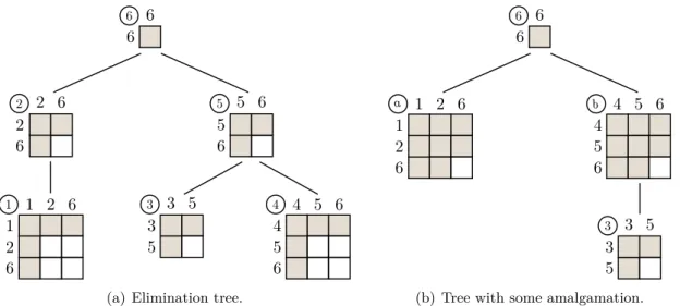
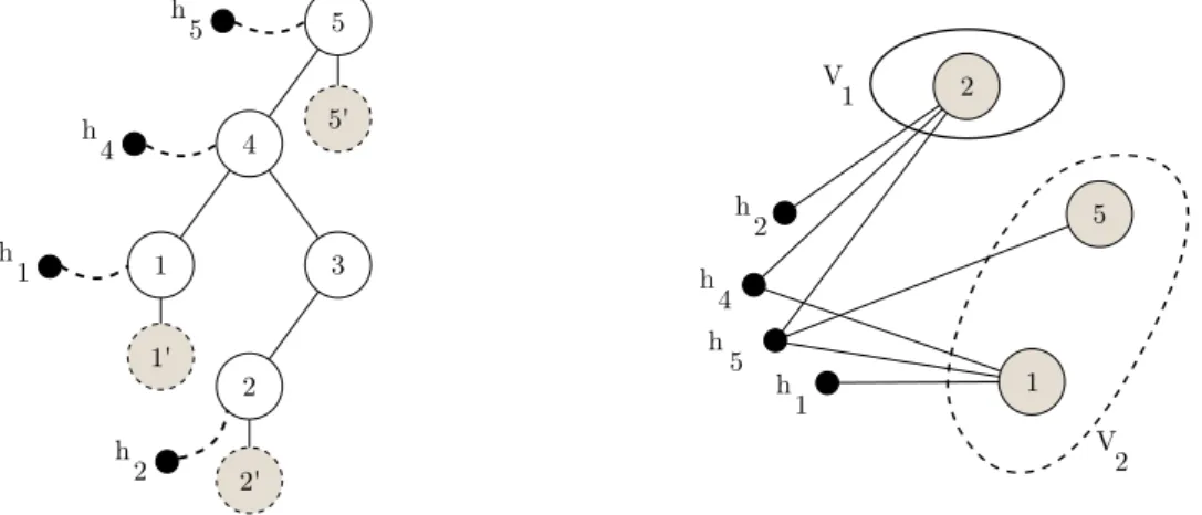
Figure

+7


Documents relatifs