Modeling SpaceWire networks with network calculus

To cite this document

: FERRANDIZ Thomas, FRANCES Fabrice, FRABOUL Christian.

Modeling SpaceWire networks with network calculus. In: 1st International Workshop on

Worst-Case Traversal Time (WCTT'11), 29 Nov 2011, Vienne, Autriche.

This is an author-deposited version published in:

http://oatao.univ-toulouse.fr/

Eprints ID: 5129

Any correspondence concerning this service should be sent to the repository administrator:

Modeling SpaceWire networks with Network Calculus

Thomas Ferrandiz

Univ. de Toulouse, ISAE France

[email protected]

Fabrice Frances

Univ. de Toulouse, ISAE France

[email protected]

Christian Fraboul

[email protected]

ABSTRACT

The SpaceWire network standard is promoted by the ESA and is scheduled to be used as the sole on-board network for future satellites. This network uses a wormhole routing mechanism that can lead to packet blocking in routers and consequently to variable end-to-end delays. As the network will be shared by real-time and non real-time traffic, network designers require a tool to check that temporal constraints are verified for all the critical messages.

Network Calculus can be used for evaluating worst-case end-to-end delays. However, we first have to model SpaceWire components through the definition of service curves. In this paper, we propose a new Network Calculus element that we call the Wormhole Section. This element allows us to better model a wormhole network than the usual multi-plexer and demultimulti-plexer elements used in the context of usual Store-and-Forward networks. Then, we show how to combine Wormhole Section elements to compute the end-to-end service curve offered to a flow and illustrate its use on a industrial case study.

Categories and Subject Descriptors

C.4 [PERFORMANCE OF SYSTEMS]: Performance attributes; C.3 [SPECIAL-PURPOSE AND

APPLICATION-BASED SYSTEMS]: Real-time and embedded systems

WCTT ’11November 29 2011, Vienna, UNK, Austria

Keywords

performance evaluation, real-time networks, SpaceWire, Net-work Calculus

1.

INTRODUCTION

SpaceWire [9], [3] is an on-board network for satellites designed by the European Space Agency and the University of Dundee. It uses high-speed serial, point-to-point links and simple routers to interconnect satellite equipment using arbitrary topologies. In the future, the ESA plans to use SpaceWire as the sole on-board network in their satellites. The idea is to use the same network for both the payload and command/control traffic. This will simplify the network architecture and reduce the costs of the satellites.

At the moment, SpaceWire provides enough bandwidth (up to 200 Mbps) to carry both types of traffic at the same time. However, in order to reduce memory size (radiation-hardened memory is very expensive), SpaceWire uses worm-hole routing to transmit the data packets across the network. The downside of this technique is that it can lead to blocked packets and thus huge variations in the end-to-end delays of those packets. Furthermore, SpaceWire does not provide built-in real-time mechanisms that guarantee the timely de-livery of urgent packets.

Thus, network designers need a tool to check that tempo-ral constraints are verified for urgent packets before SpaceWire can be used to carry command/control traffic. Using simu-lations is not possible because covering every scenario would be very long and costly. A better solution is to design an an-alytical model to compute an upper-bound on the worst-case end-to-end delay of a flow.

We proposed a first model in [5] that allowed us to com-pute such an upper-bound for a SpaceWire network. This model works well in most cases but has some limitations. As it did not require a specific model of input traffic, it was pessimistic when the network was not fully loaded.

As a consequence, we chose to create a new model based on Network Calculus theory [8]. It is a theory designed to study deterministic queueing systems which we have already successfully used in [7] to study the AFDX network. One strong point of Network Calculus is that it allows us to model the input traffic precisely by using traffic envelopes.

However, Network Calculus has been mostly used to study Internet components and not wormhole routers. As a con-sequence, the usual multiplexer and demultiplexer elements are not adequate to model a wormhole network. Thus, in Section 2, we propose a new network element we call a ”Wormhole Section”. We can then divide the path of a flow

αSin

i arrival curve of fiat the entrance of section S

αSout

i arrival curve of fi at the exit of section S

αji arrival of fiat port j

βdest

i service curve received by fiuntil its destination

(β)↑ max(sup0≤s≤tβ(s), 0)

(positive and non-decreasing upper closure)

δT δT(t) = 0 if t < T

δT(t) = +∞ if t ≥ T for any T ≥ 0

h(α, β) horizontal distance between the two positive,

non-decreasing curves α and β

Table 1: Notations used in the paper

into a series of Wormhole Sections to deduce an end-to-end service curve.

Then, in Section 3, we show how to use this element to compute an end-to-end service curve for a flow. Finally, we illustrate the use of this model on an industrial application provided by Thales Alenia Space in 4 and conclude in Sec-tion 5.

2.

THE WORMHOLE SECTION ELEMENT

A complete overview of Network Calculus would be be-yond the scope of this paper. Readers not familiar with this theory can refer to [1] for a short introduction.

Here, we just recall this fundamental theorem. Theorem 1. Concatenation of two systems

Assume that a flow traverses two systems S1 and S2 in

se-quence. Assume that S1 and S2 offer the service curves β1

and β2 respectively. Then the concatenation of the two

sys-tems offers the service curve β1⊗β2 to the flow. β1⊗β2(t) =

inf0≤s≤t{β1(t − s) + β2(s)} is the Min-Plus convolution of

β1 and β2.

This allows us to combine the network elements succes-sively traversed by a flow to obtain an end-to-end service curve offered to the flow by the network as a whole.

2.1

Assumptions

We consider a network composed of SpaceWire routers and terminals. Each terminal has only one SpaceWire inter-face but can be the source and/or destination of any number of flows. Each flow f is modeled by a source, a destination, a

path through the network and an arrival curve αf. Usually,

the arrival curve is a staircase function which gives a more precise model of the input traffic than an affine function.

Since SpaceWire routers use static routing, we consider only a static network. We also assume that the network is stable, i.e. that no link is required to transfer more data than its capacity. In Network Calculus terms, this can be

written as follows (see [2]). For each link j, we note Ij the

number of flows traversing that link and αj_i the arrival curve

of flow fiat link j. The stability condition is now:

∀j, ∀i ∈ {1, . . . , Ij}, lim

t→+∞[β j₋ Ij X i=1 αj_i](t) = +∞ (1)

Throughout the paper, we will use the notations in Ta-ble 1.

2.2

A new network element

To use Network Calculus theory, we first need to deter-mine a service curve for each element traversed by a flow. We can then compute an End-To-End (ETE) service curve using Theorem 1. However, in a wormhole network, the ser-vice offered by a router is not independent from the serser-vice offered by downstream routers. Because of the flow control, a router can output data at an average rate far inferior to its nominal capacity.

For this reason, we do not propose a classic multiplexer/ demultiplexer model of each router. Instead, we adopt a macroscopic view of the network which tries to optimize the ETE service curve of each flow while accounting for the in-terdependency between routers.

When a flow encounters interferences with other flows, the impact of each conflict is twofold. First, there is a delay when the flow is multiplexed with the interfering flow. Then, when the interfering flow is demultiplexed, the flow control mechanism will propagate its own delays backward to the studied flow.

To properly model this, we propose a new network element that we call a ”Wormhole Section” [4]. The basic idea is to divide the path followed by a flow into a serie of sections. Each section is composed of a set of successive output ports shared by the same flows. Thus, a Section corresponds to the arrival or the departure of an interfering flow from the path of the studied flow.

Each wormhole section offers a service curve that depends on the arrival curves of the interfering flows. Once we have computed the service curve of every section in the path of a flow, we can deduce the end-to-end service curve by using Theorem 1.

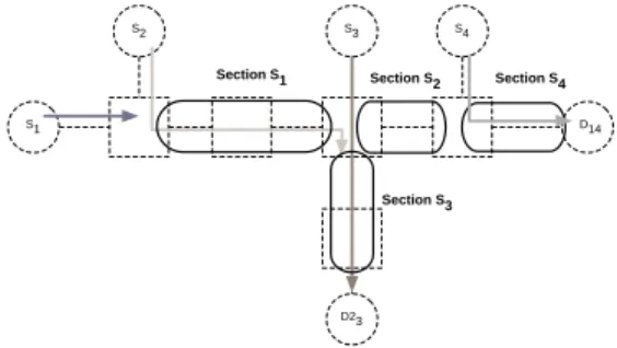
Of course, once an interfering flow has left the path of the studied flow, it will go through other wormhole sections before reaching its destination. The delays caused in those sections are those that will be carried over to the studied flow. S1 S2 S3 D23 D14 S4 Section S1 Section S2 Section S3 Section S4

Figure 1: A network divided into wormhole sections As an example, consider the network in Figure 1. Each

flow figoes from its source Sito its destination Di. When a

destination is shared by two flows i and j it is denoted Di,j.

Let us take a closer look at f1. f1has to go through three

wormhole sections (S1, S2, S4) to reach D1,4 with sections

S1 and S4 shared with other flows. S1 and S4 are thus the

two sources of direct delays for f1. In addition, since after

leaving S1, f2 traverses section S3 which it shares with f3,

S3will be another source of delay for f1but only indirectly.

As can be seen in this example, the wormhole section net-work element makes it easier to analyse the conflicts in a wormhole network. In the next section, we present a

de-tailed model of this new network element.

2.3

Section sharing

We will present the model when there is only one

interfer-ing flow. We note f1 the studied flow. f2 is the interfering

flow. fihas αSin

i as an arrival curve at the entrance of

sec-tion S. Let us assume that secsec-tion S comprises M routers.

For j = 1, . . . , M , βj is the service curve offered by the

output port of router Rj _{to the two flows. Because of the}

flow control mechanism, the amount of data which is

trans-mitted by the port may actually be inferior to βj. Thus, βj

should be seen as an intermediate parameter used to deter-mine the service guaranteed to a given flow by this section of the network. Once we have analysed the conflicts in each output port traversed by a flow, we can use Theorem 1 to compute a service curve for the section, then for the com-plete path. This end-to-end curve is now valid because it takes into account the influence of all the ports used by a

flow, including the indirect delays. As a consequence, it

represents the real end-to-end output of the network. Since all the routers in the section are shared between the two flows and no other interference occurs, we can view these

routers as a single router with service curve βS=NM_j=1βj.

SpaceWire routers use a simplified Round-Robin access scheme that guarantees that each input port gets a fair ac-ces to each output port. However, each packet can use the output port for an unlimited duration. The usual round-robin model attributes some weight to each flow and shares the bandwidth in proportion to those weights. Since the SpaceWire standard does not define such weights, we have no way of using this model and have to rely on the more pessimistic ”blind multiplexing” model [8], Theorem 6.2.1.

Thus, the service curve offered by the section to f1 is

βS1 = ( M O j=1 βj− αSin 2 )↑. (2)

(β)↑is the positive and non-decreasing upper closure of β

defined as (β)↑= max(sup0≤s≤tβ(s), 0).

βS

1 is a worst-case service curve that implies that all the

interfering flows have a higher priority than f1 and can

in-stantly preempt it. Of course, in reality the packets are not interrupted but this model ensures that we have a worst-case service curve for any possible scheduling of the packets.

2.4

Section demultiplexing

2.4.1

Limits of existing models

In a classic Store-And-Forward network model, the pack-ets are instantaneously demultiplexed. Furthermore, once a packet has left the router, the delays it can endure are not propagated backward on the network. Thus, the demulti-plexer has no impact on the delay (see [2] for example).

However, this is not true for a wormhole network. In fact,

after two flows f1 and f2 have been demultiplexed, f2 can

still have an impact on f1. This is because the flow control

mechanism will carry over the delays caused to f2 on the

end of its path backward to f1.

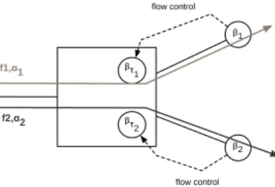
A possible way to model this phenomenon is given in [10]. In this paper, the authors consider the situation described on Figure 2. In this network, after they have been

demul-tiplexed both flows f1 and f2 have to go through a flow

βτ₂ βτ₁ β₁ β₂ flow control flow control f1,α₁ f2,α₂

Figure 2: Demultiplexing of two flows in a wormhole network

controller. Flow controller τi models the impact of the flow

control on the downstream output link on flow fi with a

service curve βτi_{. In turn, β}τi _{depends on the service curve}

of the downstream router.

The authors consider that, as far as the aggregate flow

f{1,2}is concerned, τ1 and τ2 are parallel traffic regulators.

As a consequence, the service offered to the aggregate flow

f{1,2} is β{1,2} = min(βτ1_{, β}τ2_{). This aggregate service is}

then shared between the two flows to derive the service of-fered to each individual flow.

This service is valid but is is very pessimistic. Let us

consider the example in Figure 2. The arrival curves are

affine: αi(t) = ri.t + bi and the service curves are linear:

βi(t) = Ci.t We use the following values:

f1 f2

ri(Mbps) 50 10

bi(bits) 1000 200

Ci (Mbps) 100 20

On the one hand, the service offered to f{1,2}is β{1,2}(t) =

min(C1, C2).t = C2.t. On the other hand, the arrival curve

of f{1,2} is α{1,2}(t) = α1(t) + α2(t) = r1,2.t + b1,2 with

r1,2= r1+ r2= 60 Mbps and b1,2= b1+ b2= 1200 bits.

The horizontal distance h(α{1,2}, β{1,2}) between the two curves is clearly infinite and we have to conclude that the network cannot carry both flows. This is very pessimistic because it is easy to see that this network can handle both flows.

Thus we need a new, more precise network model of worm-hole demultiplexer.

2.4.2

A new model of demultiplexing

Since both flows go in different directions in the network, we cannot determine an exact service for the aggregated flow. Each flow receives its own service but can still cause delays to the other flow thanks to the flow control mecha-nism.

The delay actually caused to an individual packet of f1 is

hard to determine because it depends on which exact con-flicts occur farther on the path of f2. However, we can de-termine an upper-bound on this delay.

In fact, the maximum delay caused by f2, which we will denote d2, is at most the maximum delivery delay from the

demultiplexer to the destination of f2. Thus,

d2= h(αSout

2 , β

dest

2 ) (3)

where αSout

2 is the arrival curve of f2 at the end of S and

β2dest the service curve offered to f2 between the end of S

Here, since we have assumed a blind multiplexing with f2 as the higher priority flow,

αSout 2 = α Sin 2  M O j=1 βj (4)

where (α  β)(t) = sup_s≥0{α(t + s) − β(s)} is the Min-Plus

deconvolution of α and β.

With this model, in the example in Figure 2 the delay

caused by f2 to f1 is only h(α2, β2) = 200₁₀7s = 10µs. As can

be seen, this model is far less pessimistic than the model from [10].

2.4.3

Complete service curve offered by a Wormhole

Section

We can combine the results from Subsection 2.3 and 2.4.2 to obtain the complete service curve offered by section S. When two flows share Section S, the service curve offered to f1 is βS1 = ( M O j=1 βj− αSin 2 )↑⊗ δh(αSout₂ ,βdest 2 ) . (5)

When there are N flows sharing a wormhole section, the service curve for flow k is

βkS= ( M O j=1 βj− N X i=1,i6=k αSin i )↑⊗ δdSk (6) with dS_k= N X i=1,i6=k di= N X i=1,i6=k h(αSout i , β dest i ).

3.

HOW TO COMPUTE AN END-TO-END

SERVICE CURVE

3.1

Model of the terminals

The first elements in the networks are the terminals them-selves. Since SpaceWire links are full-duplex, we consider that each terminal is composed of a source terminal and a destination terminal that we can model independently.

A source terminal has a FIFO input buffer that is shared by any number of applications running on the terminal. All the applications try to emit on the SpaceWire interface. For each application, we define a separate data flow. Since the flows share the output port of the terminal just like they would share the output port of a router, we consider that this output port is part of a Wormhole Section just like any routers’ output port.

A destination terminal has a reception buffer large enough to receive at least one full packet of the maximum size. It can impose a constant delay to each packet before reading it. It then reads this packet at a constant service rate, which is usually less than the speed of the links.

Thus, the service curve of a destination terminal D is

βD_{(t) = rD.(t − TD)}+ _{where rD is the service speed of D}

and TDthe delay it forces on the data.

3.2

Solving more complex interferences

The model presented in Section 2 can only be directly ap-plied when all the interfering flows arrive and depart from the same router. When it is not the case, we could simply

divide the path of the studied flow into many small worm-hole sections. We could even have a section for each router crossed by the flow.

However, this would give us a suboptimal result because we would have to count several times (once for each router) the influence of a flow that shares several consecutive routers with the studied flow. It is better to try and optimize the end-to-end service curve by combining a set of flows sharing some routers as an aggregate flow. We can then determine wormhole sections for this aggregate flow and deduce the service curves offered to it. Those service curves will then be shared between the individual flows composing the aggregate flow.

To automate this process, we use the interference patterns defined in [10] to determine the order in which the residual services are computed. The authors define three interference patterns describing how one studied flow and two interfering flows interact with one another. They also show that all conflicts, involving any number of interfering flows, can be solved once those three patterns are solved.

Below we define the interference patterns and the residual service curves for the studied flow in each case.

Let us call βj the service curve offered by router Rj. See

Table 1 for the other notations. We have di= h(αouti , β

dest

i ), i = 2, 3. We will explicit α

out i in each case since it depends on the interference between f2 and f3.

3.2.1

Nested interference pattern

R1 R2 R3 R4 R5

f1

f2 f3

Figure 3: Nested interference pattern

In this configuration (Figure 3), we first treat f1and f2as

an aggregate flow sharing the section comprising the output

port of R3with f3. Then, we consider that f1 and f2share

the section comprising the output ports of R2, R3 and R4.

The service curve offered to f1 by the section R1→ R5 is

thus β11→5=β1⊗ ([β2⊗ (β3− α33)↑⊗ δd3⊗ β 4 ] − α22)↑ ⊗ δd2⊗ β 5 (7) Here, αout 2 = α22 [β2⊗ (β3− α33)↑⊗ δd3⊗ β 4_{] and α}out 3 = α33 [(β3− α2)↑⊗ δ2]

3.2.2

Parallel interference pattern

R1 R2 R3 R4 R5

f1

f2 f3

Figure 4: Parallel interference pattern

In this configuration (Figure 4), f1shares the section

com-prising the output port of R2 with f2 and the section

com-prising the output port of R4 with f3. The other sections

R1 R2 R3 R4 R5 f1

f2a f2b f3

Figure 5: Crossed interfering pattern

The service curve offered to f1by the section R1→ R5 is

β11→5=β 1_{⊗ (β}2_{− α}2 2)↑⊗ δd2 ⊗ β3_{⊗ (β}4_{− α}4 3)↑⊗ δd3⊗ β 5 (8)

Here, α2out= α22⊗ β2and αout3 = α43⊗ β4.

3.2.3

Crossed interfering pattern

In this configuration (Figure 5), we have to split f2 into

two sub-flows f2a and f2b at R3. First, f1 shares the

sec-tion comprising the output port of R2 with f2a. Then, the

aggregate flow f1+ f3 shares the section composed of the

output port of R3 with f2b. Finally, f1 shares the section

comprising the output port of R3 andR4with f3.

In the end, the service curve offered to f1 by the section

R1→ R5 is β1→51 =β 1 ⊗ (β2− α22)↑ ⊗ ((β3− α32)↑⊗ δd2⊗ β 4 − α33)↑⊗ δd3 (9) Here, αout2 = α32  [(β3 − α33)↑⊗ δd3], α 3 2 = α22 β2, αout3 = α33 [(β3− α32)↑⊗ δd2⊗ β 4 ].

3.3

Computing the arrival curves of the

inter-fering flows

As seen above, we need to compute the arrival curves of all the interfering flows both at the beginning of the wormhole section where they meet the studied flow and at the end of this section.

For each interfering flow, the arrival curve at the beginning of the section depends on the arrival curve of the flow at the source and on the service received between the source and the beginning of the shared Wormhole Section. The arrival curve at the end of the section can then be computed from the arrival curve at the beginning of the section.

Therefore, the service received by the interfering flow is

itself dependent on other interfering flows. Furthermore,

since the service curve βdestdepends on the arrival curve of

other flows which may in turn depend on the studied flow, we risk being stuck with a circular-dependency problem.

3.4

Fixed-point method

To solve this problem, we use a fixed-point method. All the arrival curves at the sources and all the service curves of the output ports are known. In addition, the residual service curve of a port can be deduced immediately from the knowledge of the arrival curves of the conflicting flows at this port. Thus, we only have to determine the arrival curves at each output port to solve the problem.

We proceed iteratively. Let αi be the arrival curve of

flow fi at its source and αj_i be the arrival curve at port

j. We start with αj,(0)i = αi for all j. This is equivalent to

assuming that the burstiness of a flow does not increase as it traverses the network. Of course, this is an approximation.

Then, we express each αj,(n+1)i as a function of αi, of the

service curves βj_{and of any number of arrival curves α}l,(n)

k from the previous step. With each iteration, the computed arrival curves αj,(n)i increase, until they reach their real value at every point in the network.

At some point, there exists p such that ∀i, ∀j, αj,(p+1)_i =

αj,(p)i and the computation has converged toward a solution

for the system.

We have implemented and tested this method on several configurations. In each case, the computation converges in a few steps toward a solution, provided that the stability condition is respected (see 2.1).

4.

INDUSTRIAL APPLICATIONS

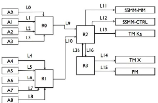
We will now present the results given by our model for an industrial configuration. This study was based on a network architecture provided by Thales Alenia Space (see Figure 6) and designed for use in an observation satellite. Our goal was to determine a worst-case end-to-end delay for each flow in the network.

4.1

Description of the network

Figure 6: Network of the industrial application As can be seen in Figure 6, the network is composed of two parts. The platform equipment on the right which includes a mass memory unit (SSMM-MM and SSMM-CTRL), a pro-cessor module (PM) and two Transmission Modules (TM Ka and TM X). The processor module monitors the other nodes and sends back commands. The mass memory is split in two parts. Data is stored in the MM module but must go through the controller unit first. Thus, other nodes send packets to the CTRL unit. This unit then processes the data during a constant delay and sends the packet to the MM unit. The CTRL unit only stores one packet at any

given time. On the left, the application terminals (A0 to

A8) represent the payload instruments. These include cam-eras and any kind of sensors. They send data packets to the CTRL unit and monitoring traffic to the PM unit.

All the links have the same capacity C = 50 M bps except

L13and L14which have a capacity Cslow= 20M bps.

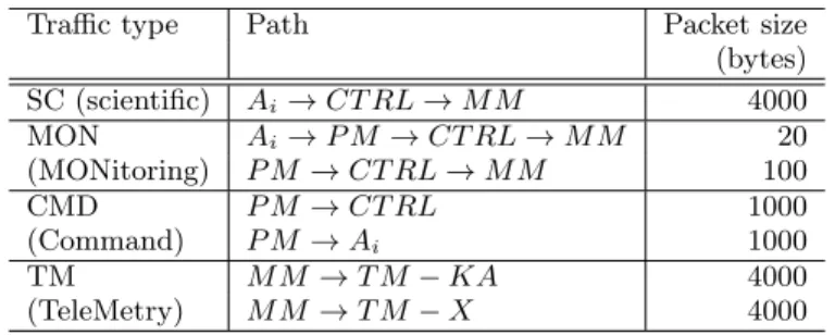
We can split the network traffic into four categories (see Table 2). The table gives the network path and the packet size for each type of traffic. Among all the nodes, only the CTRL and PM units introduce a delay for every packet they

receive. The delay is the same for both: DP M = DCT RL=

Furthermore, the PM reads data packets at 1250 bytes/s and the two TM units at 87.5 kbytes/s.

Traffic type Path Packet size

(bytes) SC (scientific) Ai→ CT RL → M M 4000 MON Ai→ P M → CT RL → M M 20 (MONitoring) P M → CT RL → M M 100 CMD P M → CT RL 1000 (Command) P M → Ai 1000 TM M M → T M − KA 4000 (TeleMetry) M M → T M − X 4000

Table 2: Network traffic

Some traffic is further divided into several flows according to the definition we used in Section 2.1. In that case, we simply take the summation of the delays for each included flow.

We implemented the model using MATLAB and the RTC Toolbox [11]. This toolbox implements all the common op-erations of Network Calculus like the min-plus convolution and deconvolution.

Our software takes a description of the network and of the network traffic as input and gives an upper-bound on the end-to-end delay of each flow as output. It implements the fixed-point method and all the computations based on the interference patterns.

4.2

Comparison with simulation results

To estimate the tightness of the bounds we computed, we compared them to the result of the simulations done by

Thales Alenia Space on this network. Those simulations

were implemented on Thales Alenia Space’s MOST simu-lator [6] that completely models the low-level behavior of SpaceWire.

The results are given in Table 3.

The critical traffic includes the CMD, TM and MON flows. The non-critical traffic includes all the SC flows.

As can be seen, the maximum delays observed during the simulations and the upper-bound computed using Network Calculus are in the same order of magnitude. This shows that our methods is not too pessimistic and gives exploitable results for a network designer.

It is also worth noting that we do not know if the max-imum observed delay is the worst-case delay or not. The real worst-case delay may be higher and, thus, closer to the bound we computed because worst-case delays are extremely rare events that are hard to observe with simulations.

For the non-critical traffic, the bound is less tight but it is not a problem fot this type of traffic. The only thing we are interested in for non-critical traffic is whether the bound is finite. If it is, it shows that the network is able to carry all the traffic in a finite time. This knowledge is sufficient for

Traffic type MOST NetCal

non-critical 16.6 102

critical 145 439

Table 3: Comparison between MOST results and our model (all results are in ms)

non-critical traffic.

5.

CONCLUSION

In this paper, we have defined a new Network Calculus el-ement that can be used to model a SpaceWire network more accurately than the usual multiplexer and demultiplexer el-ements. We call this new element a Wormhole Section since it represents a part of the path followed by a flow. The Wormhole Section should allow us to obtain tighter bounds by considering successive routers as only one element.

Furthermore, we also described a new way to compute the delay caused by a flow leaving a wormhole section. We showed on a simple example that our method is a lot less pessimistic than existing demultiplexer models for a worm-hole network.

Our model is based on the Network Calculus theory and uses the interference patterns defined in [10] by Qian et al to model complex dependencies with the interfering flows. Furthermore, it uses a fixed-point computation to solve cir-cular dependencies between the arrival curves of the various flows.

We evaluated our model on an industrial configuration in Section 4. On this example, we showed that the bounds obtained by our method are close to the maximum delay observed during the simulations.

In the future, we plan to pursue two objectives. The first goal is to formally prove the convergence of the fixed-point method use in Section 3. The second will be to find a more realistic model of the non-preemptive section sharing. This should allow us to tighten the upper-bounds even more.

Acknowledgment

This work was supported by a PhD grant from the CNES and Thales Alenia Space.

6.

REFERENCES

[1] J. L. Boudec and P. Thiran. A short tutorial on network calculus. i. fundamental bounds in

communication networks. Circuits and Systems, 2000. Proceedings. ISCAS 2000 Geneva. The 2000 IEEE International Symposium on, 4, 2000.

[2] R. L. Cruz. A calculus for network delay, part i: Network elements in isolation. IEEE Transactions on Information Theory, 37(1), Jan 1991.

[3] ECSS. Spacewire – links, nodes, routers and networks. Aug 2008.

[4] T. Ferrandiz, F. Frances, and C. Fraboul. Using network calculus to compute worst-case end-to-end delays in spacewire networks. ECRTS 11

Work-in-Progress session.

[5] T. Ferrandiz, F. Frances, and C. Fraboul. A method of computation for worst-case delay analysis on spacewire networks. Industrial Embedded Systems, 2009. SIES ’09. IEEE International Symposium on, 2009. [6] P. Fourtier, A. Girard, A. Provost-Grellier, and

F. Sauvage. Simulation of a spacewire network. Proceedings of the International SpaceWire Conference 2010, Oct 2010.

[7] F. Frances and C. Fraboul. Using network calculus to optimize the afdx network. ERTS 2006 : 3rd European Congress ERTS Embedded real-time software, Jan 2006.

[8] J. LeBoudec and P. Thiran. Network calculus a theory of deterministic queuing systems for the internet. Springer Verlag, (LNCS 2050), Apr 2004.

[9] S. M. Parkes and P. Armbruster. Spacewire: A spacecraft onboard network for real-time

communications. IEEE-NPSS Real Time Conference, (14), Feb 2005.

[10] Y. Qian, Z. Lu, and W. Dou. Analysis of worst-case delay bounds for best-effort communication in wormhole networks on chip. Proceedings of the 2009 3rd ACM/IEEE International Symposium on Networks-on-Chip-Volume 00, 2009.

[11] E. Wandeler and L. Thiele. Real-Time Calculus (RTC) Toolbox.