To cite this document:
Dang, Dinh Khanh and Mifdaoui, Ahlem Timing Analysis of
TDMA-based Networks using Network Calculus and Integer Linear Programming.
(2014) In: IEEE 22nd International Symposium on Modeling Analysis and Simulation of
Computer and Telecommunication Systems (MASCOTS), 9 September 2014 - 11
September 2014 (Paris, France).
O
pen
A
rchive
T
oulouse
A
rchive
O
uverte (
OATAO
)
OATAO is an open access repository that collects the work of Toulouse researchers and
makes it freely available over the web where possible.
This is an author-deposited version published in:
http://oatao.univ-toulouse.fr/
Eprints ID: 11568
Any correspondence concerning this service should be sent to the repository
administrator:
[email protected]
Timing Analysis of TDMA-based Networks using
Network Calculus and Integer Linear Programming
Dinh-Khanh Dang
University of Toulouse-ISAE [email protected]Ahlem Mifdaoui
University of Toulouse-ISAE [email protected]Abstract—For distributed safety-critical systems, such as
avionics and automotive, shared networks represent a bottleneck for timing predictability, a key issue to fulfill certification require-ments. To control interferences on such shared resources and guarantee bounded delays, the Time Division Multiple Access (TDMA) protocol is considered as one of the most interesting arbitration protocols due to its deterministic timing behavior and fault-tolerance features. This paper addresses the problem of computing the worst-case end-to-end delay bounds for traffic flows sharing a TDMA-based network using Network Calculus. First, we extend classic timing analysis to integrate the impact of non-preemptive message transmission and various service policies in end-systems, e.g., First In First Out (FIFO), Fixed Priority (FP) and Weighted Round Robin (WRR). Afterwards, the proposed models are refined using Integer Linear Programming (ILP) to obtain tighter end-to-end delay bounds. Finally, this general analysis is illustrated and validated in the case of a TDMA-based Ethernet network for I/O avionics applications. Results show the efficiency of the proposed models to provide stronger guarantees on system schedulability, compared to classic models.
I. INTRODUCTION
For safety-critical applications, such as avionic and auto-motive, guarantees on worst-case behavior are key issues to fulfill certification requirements. The main difficulty to conduct such an analysis arises from the increasing complexity of new generation safety-critical systems. These new systems are generally based on shared resources, such as networks for distributed end-systems. These shared networks represent the bottleneck for performance and timing predictability. To control interferences and guarantee bounded access delays, various arbitration mechanisms can be integrated.
Among existing arbitration protocols, Time Division Mul-tiple Access (TDMA) has been successfully used in various embedded networks, such as FlexRay [3] for automotive and more recently Time Triggered Ethernet [6] for avionics. TDMA consists of partitioning the network access over time, and assigning it to only one end-system during any particular time slot. The use of TDMA to control medium-access has many advantages due to its deterministic timing behavior and its contention-free and fault-tolerance features. However, TDMA may lead at the same time to increasing communication latencies, thus requiring real-time constraints be verified. To deal with the worst-case performance analysis of such systems, an appropriate timing analysis to provide worst-case end-to-end delay bounds has to be considered.
Many challenges arise from conducting such an analysis. First, safety-critical systems are based on non-preemptive
communication where a message transmission cannot straddle two slots, and consequently if the remaining time during a slot is not enough for a complete transmission, then the message has to wait for the next slot. Second, the communication networks in such systems are used to transmit traffic flows with different temporal constraints. This implies guaranteeing a delay bound for each data-type and proving the temporal isolation between flows. Third, the end-systems sharing the TDMA-based network implement service policies, such as First In First Out (FIFO), Fixed Priority (FP) and Weighted Round Robin (WRR) policies. The impact of such policies on the analysis of worst-case end-to-end delays needs to be integrated.
Among analytical methods to conduct worst-case perfor-mance analysis of distributed networks, Network Calculus [8] is well adapted to controlled traffic sources and provides upper bounds on delays for traffic flows. It has been used in many application fields, such as wireless sensor networks [5] [7], avionics [9] and space networks [4]. In the area of timing analysis for TDMA-based systems, some interesting work based on Network Calculus has been proposed [5] [7] [10]. These approaches are mainly based on fluid flow models which may result in optimistic end-to-end delay bounds, i.e., less than the delays that may actually occur. This fact may provide guarantees for messages that will actually miss their deadlines in the worst-case when considering packet flow models.
The contributions of this work are: (i) Efficient timing analysis using Network Calculus for a packet flow model under FIFO, FP and WRR policies sharing a TDMA-based network. To our knowledge, WRR modeling under these conditions has not been treated in the literature; (ii) Refining the proposed models for the different service policies using Integer Linear Programing (ILP) to compute tighter end-to-end delay bounds; (iii) The validation of such timing analyses in the case of a TDMA-based Ethernet network for I/O avionics applications. The efficiency of the proposed models to provide stronger guarantees on system schedulability is proved, with reference to classic models.
In the next section, we describe the basic concepts of Network Calculus framework, and we review the most relevant work in the area of timing analysis using Network Calculus of TDMA-based networks. Afterwards, the timing analysis of TDMA-based networks under various service policies is tackled as follows. First, the system modeling and schedula-bility analysis methodology are presented in Section III. Then, extended service curves based on packet flow models under various service policies are detailed in Section IV, and refined
using ILP in Section V. Finally, the validation of such timing analysis is illustrated within a realistic avionic application.
II. BACKGROUND ANDRELATEDWORK
A. Network Calculus Framework
The timing analysis of TDMA-based networks detailed in this paper is based on Network Calculus theory [8], providing upper bounds on delays and backlogs. Delay bounds depend on the traffic arrival described by the so called arrival curve
α, and on the availability of the traversed node described by the so called minimum simple or strict service curveβ. The definitions of these curves are explained as following.
Definition 1. (Arrival Curve) a functionα is an arrival curve
for a data flow with an input cumulative function R, such that R(t) is the number of bits received until time t, iff:
∀t, s ≥ 0, s ≤ t, R(t) − R(s) ≤α(t − s)
Definition 2. (Simple service curve) The function β is the
minimum simple service curve for a data flow with an input cumulative function R and output cumulative function R∗ iff:
R∗≥ R ⊗β where( f ⊗ g)(t) = inf0≤s≤t{ f (t − s) + g(s)}
Definition 3. (Strict service curve) The function β is the
minimum strict service curve for a data flow with an input cumulative function R and output cumulative function R∗, if for any backlogged period]s,t]1, R∗(t) − R∗(s) ≥β(t − s).
The delay bound D is the maximum horizontal distance betweenα andβ called h(α,β); whereas the backlog bound
B is the maximum vertical distance called v(α,β). Finally, to compute delay bounds of individual traffic flows, we need the residual service curve according to the following theorem.
Theorem 1. (Residual service curve - Blind Multiplex) [1]
let f1 and f2 be two flows crossing a server that offers a strict service curveβ such that f1isα1-constrained, then the
residual service curve offered to f2is: β2= (β−α1)↑
where f↑(t) = max{0, sup0≤s≤t f(s)}
B. Timing Analysis of TDMA-based Networks
A timing analysis of TDMA-based systems using Network Calculus aims to provide a method to compute end-to end delay bounds of transmitted messages. These obtained values are then compared to message deadlines to verify system schedulability.
In [5] [7], the authors applied Network Calculus to provide real-time guarantees for Wireless Sensor Networks (WSNs). The former work proposed an optimization approach to design a TDMA arbiter for generic sink-tree WSNs; whereas the latter focused on performance analysis of such networks considering the sink mobility. Another interesting work in this area was proposed by Wandeler et al. [10] where the authors proposed an approach to find the optimal cycle length as well as
1]s,t] is called backlogged period if R(τ) − R∗(τ) > 0,∀τ∈]s,t]
the minimum required bandwidth of TDMA resource under FIFO and FP service policies in end-systems. These different approaches are based on a fluid flow model which may lead to optimistic end-to-end delays when considering a packet flow model with non-preemptive message transmission.
In this paper, we provide extended timing analysis of such systems to integrate the non-preemption of message transmis-sion under various service policies such as FIFO, FP and WRR. Further, we refine the proposed models using Integer Linear Programming (ILP), using the same idea introduced in [2] for tandem networks under FIFO multiplexing, to compute tighter end-to-end delay bounds. Finally, we discuss the possible impact of such timing analysis in the case of a TDMA-based Ethernet network for I/O avionics applications. The efficiency of our proposed models to provide stronger guarantees on system schedulability compared to classic models is validated.
III. TIMINGANALYSISMETHODOLOGY
To conduct timing analysis of TDMA-based Networks us-ing Network Calculus, we first define the system scenario and assumptions. Then, we present the considered schedulability test and detail models of traffic flows, end-systems and the TDMA arbitration protocol.
A. System Scenario and Assumptions
The considered end-systems generate messages indepen-dently and transmit their generated traffic flows on the shared medium under various service policies: FIFO, FP or WRR.
The inter-communication between these end-systems is based on a TDMA network and follows a static TDMA schedule. A TDMA schedule is defined as a sequence of time slots repeated each cycle with a fixed duration, called c. During each cycle, each end-system can only transmit during a predetermined time interval, called TDMA time slot s. We consider the general case where the time slots associated to end-systems have not necessarily equal durations. The message transmission on this TDMA-based network is non-preemptive. Consequently, if the remaining time during a slot is insufficient for a complete message transmission, then the message has to wait for the next slot. Hence, the cycle duration is as follows:
c=
M
∑
k=1
sk+ tsync (1)
where M is the number of end-systems, and tsync the duration
of the synchronization phase.
B. Sufficient Schedulability Test
Using Network Calculus, an upper bound on end-to-end delay of each transmitted message m, Deedm , is computed and then compared to its respective temporal deadline, Dlm.
Hence, this schedulability test results in a sufficient but not necessary condition due to the pessimism introduced by the upper bounds. Nevertheless, we can still infer the traffic schedulability as follows:
∀m ∈ messages,
Deed
The end-to-end delay of each transmitted message m con-sists mainly of three parts:
• arbitration delay that corresponds to the maximum waiting time since the arrival instant of the mes-sage until it starts being transmitted on the network medium. This delay is due to interference caused by other messages from the same end-system, and the waiting time due to TDMA arbitration protocol; • transmission time that corresponds to the
communica-tion time of the message on the medium; it depends on the message size and the medium transmission capacity;
• propagation delay needed to propagate a signal from a source to its final destinations. In our case, this delay is considered insignificant.
C. System Modeling
To compute upper bounds on end-to-end delays of transmit-ted messages using Network Calculus, we need to model each message flow to compute its maximum arrival curve, and the behavior of end-systems and the TDMA arbitration protocol to compute the minimum service curve.
The characteristics of an aggregate traffic flow figenerated
by an end-system are defined as (ni, Ti, Dli, Li, ei) for the
number of message flows, the message period (and minimum inter-arrival time for sporadic flow), deadline (equal to Ti
unless otherwise explicitly specified), frame size integrating the protocol overhead and delivery time (i.e., ei= Li/B where
B is the medium transmission capacity), respectively.
The arrival curve of traffic flow i, based on a packetized model is as follows.
αi(t) = niLi⌈
t Ti
⌉ (2)
For end-systems and TDMA protocol modeling, first we present existent classic models based on a fluid flow model for FIFO and FP policies. However, to our best knowledge, no model for WRR policy combined with TDMA protocol currently exists. These models will be then extended in the next sections to integrate the impact of non-preemptive message transmission.
The classic service curve for a fluid flow model when FIFO policy is implemented in the end-system has the following analytical expression: βc,s(t) = B max(⌊ t c⌋s,t − ⌈ t c⌉(c − s)), ∀t ≥ 0 (3)
The main idea is based on the fact that an end-system with a time slot s may not have access to the shared network during at maximum c− s. After this maximum duration, the end-system has exclusive access to the medium during its time slot
s to transmit with the medium transmission capacity, B. When
considering FP policy, each traffic flow will be transmitted before all lower priority flows and after all higher priority flows. Consider N traffic flows f1, .., fN where fi has higher
priority than fj if i< j. The residual service curve offered to
traffic flow fi using Theorem 1 has the following analytical
expression:
βi(t) = (βc,s(t) −
∑
1≤ j≤i−1αj(t))↑ (4)
D. Computing Upper Bounds on End-to-End Delays
Upper bounds on end-to-end delays can easily be computed as the maximum horizontal distance between the maximum arrival curve of the traffic and the minimum service curves guaranteed by each end-system when implementing FIFO, FP or WRR policies.
Consider an end-system generating N traffic flows and each flow fi characterized with the maximum arrival curve αi(t),
the upper bound end-to-end delay Deedi associated to flow fi
depends on the implemented service policy in the end-system: • with FIFO policy, Deed
i is the upper bound on
end-to-end delay guaranteed to the aggregate traffic flow generated by the same end-system when considering the minimum service curveβ(t). Hence,
∀i Deedi = h(α,β) whereα(t) = N
∑
i=1
αi(t) (5)
• with FP and WRR policies, Deedi is the maximum hor-izontal distance between the maximum arrival curve
αi(t) and the guaranteed residual service curve βi.
Hence,
∀i Deedi = h(αi,βi) (6)
IV. PACKETSERVICECURVES USINGNETWORK CALCULUS
In this section, the extended service curves based on a packet flow model are detailed and proved under various service policies, i.e., FIFO, FP and WRR.
A. FIFO Policy
The maximum waiting time to access the medium and the lower bound of offered TDMA time slot have to be adjusted in case of non-preemptive message transmission, and then used to extend the service curve guarantee.
Consider an end-system with a TDMA time slot s during each TDMA cycle c. This end-system generates N traffic flows with associated maximum and minimum delivery times
emax and emin, respectively. Based on the worst-case scenario
illustrated in Figure 1, the corresponding parameters are as following.
−
ε
−
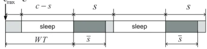
Figure 1. Worst case scenario with FIFO policy
• The maximum waiting time W T occurs when the first message of a backlogged period has a maximum delivery time
emax and arrives just at the instant when the remaining time
during the current slot is slightly less then the required delivery time, i.e., emax−ε(0 <ε<< 1). In this case, the message has
to be delayed until the next slot and the maximum waiting time is then W T= emax+ c − s instead of c − s in the classic model.
• The lower bound of offered TDMA time slot s depends on message flows characteristics. If generated messages are homogeneous, i.e., all the messages have the same delivery time e, then the end-system can send at maximum ⌊s
e⌋
messages during its respective time slot s. Else, the idle time is always less than emax and the lower bound of offered TDMA
time slot is always greater than emin. Hence, s is as follows:
s= (
⌊s
e⌋e if emax= emin= e
max{s − emax, emin} Otherwise
(7)
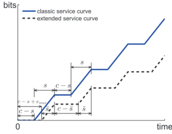
The maximum waiting time W T may occur only at the beginning of the backlogged period. Then, during the next cycles the node may wait at most c− s to access to the network and transmit messages. Hence, the strict service curve guaranteed in this case isβ(t) =βc,s(t − (W T − (c− s))) which represents the curve shifted to the right with the positive duration W T− (c − s) of βc,s(t) defined in Eq. 3.
This is explicitly defined in the following theorem. The corresponding proof is detailed in Appendix VIII-A.
Theorem 2. Consider an end-system having a lower bound
of offered time slot s, generating N traffic flows and imple-menting a FIFO policy. The offered strict service curve when considering non-preemptive message transmission is:
β(t) =βc,s(t − W T + (c − s)), ∀t ≥ 0 where W T= emax+ c − s, and s= ( ⌊s
e⌋e if emax= emin= e
max{s − emax, emin} Otherwise
The extended service curve for a packet flow model is illus-trated in Figure 2. Notice the extended service curve is lower than the classic one, described in Eq. 3. This difference leads to greater delay bounds, mainly due to the non-preemptive message transmission.
B. FP Policy
As for the FIFO policy case, the maximum waiting time to access to the medium and the lower bound of offered TDMA
time slot for transmission have to be adjusted in case of
non-preemptive message transmission. First, we compute the offered service curve for aggregate traffic flow f≤i including traffic flows f1,.., fi with priorities higher or equal to i. Then,
we deduce the individual service curve for each traffic flow
fi applying Theorem 1. Based on the worst-case scenario
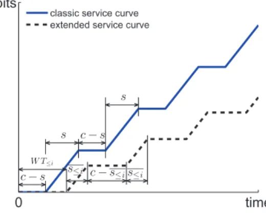
illustrated in Figure 3, the corresponding parameters are as follows:
• The maximum waiting time W T≤i occurs when the first message of the aggregate message flow f≤i arriving at the
0 time bits c − s c − s + emax c − s s c − ¯s ¯s ¯ s s
classic service curve extended service curve
Figure 2. Classic vs extended service curves with FIFO policy ε ≤ ≤ −
−
≤ ≤ ε < ≤ − ≤Figure 3. Worst case scenario with FP policy
beginning of a backlogged period and having a maximum delivery time e1≤ j≤imax is blocked during the transmission time
of a message with lower priority and maximum delivery time. This blocking time corresponds to eimax< j≤N−ε(0 <ε<< 1).
Furthermore, after that blocking time, the remaining time during the current slot is slightly less then the required delivery time of the considered message and is equal to e1≤ j≤imax −ε(0 <
ε<< 1). In this case, this message has to wait until the next slot to be transmitted. The maximum waiting time is then bounded by eimax< j≤N+ e1≤ j≤imax + c − s. However, if TDMA time
slot s< eimax< j≤N+ e1≤ j≤imax , then the maximum waiting time is
reduced to one cycle c(= s + c − s). Hence, for aggregate flow
f≤i, the maximum waiting time is as follows:
W T≤i= min(eimax< j≤N+ e1≤ j≤imax + c − s, c) (8)
• The lower bound of offered TDMA time slot associated to aggregate message flow f≤i, called s≤i, can be deduced from Eq. 7 by considering only aggregate flow f≤iinstead of all the generated flows. Hence, s≤i associated to aggregate flow f≤i is as follows: s≤i= ( ⌊s e⌋e if e 1≤ j≤i
max = e1≤ j≤imin = e
max(e1≤ j≤imin , s − e1≤ j≤imax ) Otherwise
(9)
The extended service curve with FP policy is defined in the following theorem and the mathematical proof is detailed in Appendix VIII-A.
Theorem 3. Consider aggregate traffic flow f≤i having a
lower bound of offered TDMA time slot s≤i, transmitted by an
end-system implementing FP policy. The strict service curve guaranteed to f≤i when considering non-preemption feature
is:
where
W T≤i= min(eimax< j≤N+ e1≤ j≤imax + c − s, c),
and s≤i= ( ⌊s e⌋e if e 1≤ j≤i
max = e1≤ j≤imin = e
max(e1≤ j≤imin , s − e1≤ j≤imax ) Otherwise
Hence, using Theorems 1 and 3, the residual service curve offered to message flow fi is as follows:
βi(t) = (βc,s≤i(t − W T≤i+ (c − s≤i)) −
i−1
∑
j=1
αj(t))↑ (11)
This extended service curve is illustrated in Figure 4. Extended service is lower than the classic service which leads to greater delay bounds due to the non-preemptive message transmission. 0 time bits c − s W T≤i c − s s c − s≤is≤i s≤i s
classic service curve extended service curve
Figure 4. Classic vs extended service curves with FP policy
C. WRR Policy
As a first step, we detail a service curve model for WRR policy combined with TDMA protocol for a fluid flow model, which to our knowledge has not been investigated in literature. Then, we extend this model to the packet flow model.
−
− +
−
Figure 5. Access-time distribution with preemptive WRR over TDMA
As illustrated in Figure 5, for each flow fi in an
end-system, we consider a respective access time to the medium, called wi during each WRR round, where ∑Ni=1wi= s. During
a backlogged period of a flow fi, the maximum waiting time
occurs when it is blocked by all other flows having their back-logged period simultaneously. Hence, the maximum waiting
time is bounded by ∑Nj=1, j6=iwj+ c − s = c − wi. Then, flow fi
receives the right to send during its respective access time wi.
This behavior is repeated according to weighted round-robin scheduling and the analytical expression is given in Theorem 4.
Theorem 4. The strict service curve for flow fitransmitted by
a node implementing a preemptive WRR combined with TDMA system, with a respective access time to the medium wi such
that ∑N
i=1
wi= s is
βi(t) =βc,wi(t) (12)
Proof: During any duration c, flow fi can access and
transmit messages during at least wi. Hence, the minimum
service curve of fi is given byβi(t) =βc,wi(t).
Then, we extend this first model to integrate the non-preemption. This condition impacts the maximum waiting time and the respective access time to the medium wi for each flow
fi. As shown in Figure 6,
ε
−
− = ≥ + − + − = − = −Figure 6. Worst case scenario with WRR policy
• The respective access time to the medium of flow
fi corresponds to the amount of time to transmit
completely⌊wi
ei⌋ messages within a slot duration that
is equal to wi= ⌊weii⌋ ∗ ei.
• The maximum waiting time occurs when flow fistarts
its backlogged period and it is blocked by all the other backlogged flows during the slot. The maximum
waiting time also has to integrate the remaining idle
time between two slots due to flow fk as shown
in Figure 6, which is slightly less than emax.
Con-sequently, the flow has to be delayed to the next slot. Hence, the maximum waiting time is bounded by emax+ c − s + ∑Nj=1, j6=iwj. It is worth noting that
during any period c= emax+ c − s + ∑1≤ j≤Nwj, the
backlogged flow fi can transmit at least ⌊wei
i⌋
mes-sages.
The analytical expression of this offered service curve in this case is given in Theorem 5 and the proof is detailed in Appendix VIII-B.
Theorem 5. The strict service curve for fi, transmitted by
a node implementing a non-preemptive WRR combined with TDMA system is βi(t) =βc,wi(t) (13) where wi= ⌊ wi ei ⌋ ∗ ei, and c = emax+ (c − s) + N ∑ j=1 wj.
D. Numerical Results
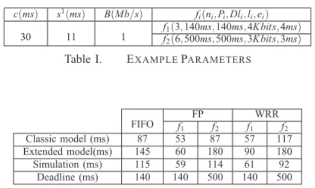
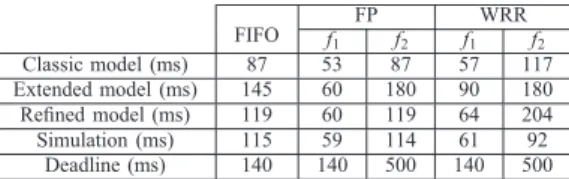
We consider the example described in Table I to compute end-to-end delay bounds for traffic flows generated by node 1 when implementing FIFO, FP or WRR service policies, and having an associated slot s1= 11 during a cycle c = 30. For WRR, a heuristic weight allocation is considered based on traffic rates. The obtained upper bounds on end-to-end delays under FIFO, FP and WRR scheduling policies with the classic and extended models are described in Table II, with reference to worst-case simulation results.
c(ms) s1(ms) B(Mb/s) f
i(ni, Pi, Dli, li, ei)
30 11 1 ff12(3, 140ms, 140ms, 4Kbits, 4ms)(6, 500ms, 500ms, 3Kbits, 3ms)
Table I. EXAMPLEPARAMETERS
FIFO f1 FP f2 f1WRRf2
Classic model (ms) 87 53 87 57 117 Extended model(ms) 145 60 180 90 180 Simulation (ms) 115 59 114 61 92
Deadline (ms) 140 140 500 140 500
Table II. DELAYS WITH CLASSIC AND EXTENDED MODELS
Upper bounds on end-to end delays obtained with classic models under the different service policies infer that the system schedulability is verified. However, with reference to worst-case simulation results, we notice that classic models lead to optimistic upper bounds on end-to end delays under the different service policies. Consequently, ignoring the non-preemptive message transmission in the model may lead to wrong decision concerning system schedulability.
However, we notice that upper bounds on end-to-end delays obtained with extended models are always greater than worst-case simulation results, and infer that the system schedulability is not proved under FIFO policy, where the delay is greater than the deadline.
V. REFINEDSERVICECURVES WITHINTEGERLINEAR PROGRAMMING
To compute tighter upper bounds on delays, we refine in this section the service curves under the different policies based on ILP. First, analytical formulations of the optimization problems corresponding to the service policies are detailed. Then, the obtained parameters are integrated in the refined service curves.
A. Problem Formulation for FIFO and FP policies
Before going through the analytical formulation of the optimization problem, consider again the example in Table I under FIFO multiplexing to show the pessimism of the considered offered TDMA time slot allocated to node 1 in the extended model. According to Eq.7, the lower bound of offered
TDMA time slot is s= max{s − e1, e2} = 7ms.
However, there are actually three possible scenarios to transmit messages of traffic flows f1and f2during the TDMA time slot of node 1: (i) 2 messages of flow f1 and 1 message of flow f2, (ii) 2 messages of flow f1, (iii) 1 message of flow
f1 and 2 messages of flow f2, (iv) 3 messages of flow f2. As we can see, the minimum offered TDMA time slot is actually equal to 8 ms which corresponds to scenario (ii). This value is consequently greater than the computed one with Eq.7, 7ms. Hence, we can clearly see that this computed value may lead to pessimistic delay bounds, i.e., more than the worst-case delays that may actually occur.
To obtain the minimum duration of the offered TDMA time slot, we first formulate the problem under FIFO multiplexing. Then, we extend this formulation under FP multiplexing. Our objective is to find the minimum of offered TDMA time slot s.
For each end-system generating N traffic flows, we consider
xi the number of messages of traffic flow fi that can be
transmitted within a time slot s. The respective ILP problem is as follows: minimize s= ∑N i=1xi∗ ei (14) subject to: ∑Ni=1xi∗ ei≤ s (14a) s− (∑Ni=1xi∗ ei) < emax (14b) xi∈ N, 1 ≤ i ≤ N (14c) where,
• the objective is to minimize the offered TDMA time slot when transmitting a variable number of messages of the different flows (1≤ i ≤ N) in order to maximize the remaining time and cover the worst-case scenario; • constraint (14a) guarantees that the offered TDMA time slot s is smaller than the allocated TDMA time slot s;
• constraint (14b) guarantees that the remaining time with the minimum offered TDMA time slot is smaller than the maximum message delivery time emax;
• constraint (14c) guarantees that the number of trans-mitted messages xi of each traffic flow fi is
non-negative integer.
The minimum offered TDMA time slot that results from this ILP problem s is integrated in the extended service curve model described in Theorem 2 to obtain the refined service curve model detailed in the following corollary.
Corollary 1. Let consider an end-system having the minimum
offered TDMA time slot s, a refined strict service curve guaranteed on TDMA-based network under FIFO multiplexing is
β(t) =βc,s(t − W T + (c − s))
This ILP formulation can be easily extended under FP policy. To find the minimum offered TDMA time slot s≤i of the aggregate flow f≤i, we need to consider only the subset of traffic flows { f1, f2, .., fi} instead of all traffic flows N in
the ILP problem formulation (14). The obtained minimum offered slot s≤iis then integrated in the extended service curve
described in Theorem 3 to obtain the refined service curve detailed in the following corollary.
Corollary 2. Let consider aggregate flow f≤ihaving the
mini-mum offered TDMA time slot s≤i, a refined strict service curve
guaranteed on TDMA-based network under FP multiplexing is β≤i(t) =βc,s≤i(t − W T≤i+ (c − s≤i))
Using Theorem 1 and Corollary 2, a refined service curve for flow fi is given by:
βi(t) = (β≤i(t) −
i−1
∑
j=1
αj(t))↑ (15)
The optimization problem can be seen as a bin-packing problem which is known to be NP-hard. However, from a practical point of view, if the number of traffic flows is not too large (less than 100), we can solve this optimization problem efficiently in a short time.
B. Problem Formulation for WRR policy
First, we show through the example described in Table I that we can obtain tighter delay bounds if we accurately select the respective transmission time w for each flow. Then, we try to find the best slot-distribution between the different flows to respect their stability condition and to reduce the delay bounds pessimism.
Revisiting the example, we simply transformed the respec-tive access times w1= 7.7, w2= 3.9 of flows f1and f2 to the refined weights w1= 4 (1 message m1), w2= 3 (1 message m2) for non-preemptive transmission. This transformation leads to the unfair treatment for flow f1. However, if we consider instead w1= 8 (2 message m1) for flow f1, then the delay bound becomes D1= 64 which is lower than the one obtained with the extended model. This change shows the impact of time-access distribution between the flows on the delay bounds tightness. Hence, we will try to find the most accurate respective access time for each flow using ILP.
The ILP formulation for WRR is as follows: minimize ∑Ni=1|wi− xi∗ ei| (16) subject to: emax+ c − s + ∑Ni=1xi∗ ei= c (16a) ∑Ni=1xi∗ ei≤ s (16b) xi∗ ei∗ B c ≥ ri, ∀1 ≤ i ≤ N (16c) xi∈ N+, ∀1 ≤ i ≤ N (16d) where,
• the objective function is to minimize the difference between the offered access times in preemptive and non-preemptive cases for all flows;
• constraint (16a) guarantees the respect of the maxi-mum round robin cycle duration c;
• constraint (16b) guarantees that the sum of all respec-tive access time is smaller than the initial slot duration; • constraint (16c) is needed to guarantee the stability condition of any flow i where the offered service rate has to be greater than the traffic rate ri.
• constraint (16d) guarantees that the number of trans-mitted messages xi of each traffic flow fi is a positive
integer.
Let (x∗1, x∗2, .., x∗N) be the optimal solution of the optimiza-tion problem above. Flow fi is allowed to transmit up to
x∗i messages during each WRR round. Hence, the respective access time is wi= x∗i∗ ei to obtain the refined service curve
defined in the following corollary.
Corollary 3. The strict service curve guaranteed on
TDMA-based network under non-preemptive WRR multiplexing is βi(t) =βc,wi(t) (17)
where wi= x∗i∗ ei and c= emax+ c − s + ∑Nj=1wj
C. Numerical Results
We consider again the example in Table I and recompute the obtained delay bounds for traffic flows f1 and f2 under FIFO, FP and WRR policies using the refined service curve models. The obtained delay bounds using refined service curve models are described in Table III.
FIFO f1 FP f2 f1WRRf2 Classic model (ms) 87 53 87 57 117 Extended model (ms) 145 60 180 90 180 Refined model (ms) 119 60 119 64 204 Simulation (ms) 115 59 114 61 92 Deadline (ms) 140 140 500 140 500
Table III. DELAY BOUNDS WITH DIFFERENT MODELS
As we can see, the delay bounds with the refined model are tighter than the extended model under FIFO, FP and WRR multiplexing and greater than worst-case simulation results. Further, the new upper bounds with refined models infer system schedulability under FIFO, which was not proved with the extended model. This fact highlights the importance of the used model and its impact on the system schedulability guarantees.
VI. VALIDATION
In this section, we evaluate the efficiency of our proposed analytical framework for timing analysis of safety-critical systems based on TDMA arbitration through a realistic avionic case study. The impact of the analytical model on the system schedulability is discussed herein with reference to simulation results.
A. Case Study
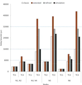
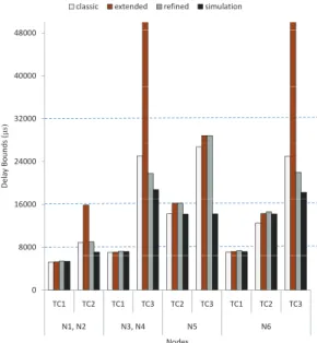
Our case study is a representative avionic sensors/actuators network based on TDMA-based Ethernet at 100Mbps inter-connecting seven I/O modules and an avionic controller, as illustrated in Figure 7. We consider three scenarios where all
the nodes use either FIFO, FP or WRR. We have an equal time slots allocation among the different I/O modules where TDMA time slot duration s= 256 µs and TDMA cycle c= 1792µs. There are three types of aggregate traffic flows generated by the different I/O modules and described in Table IV. Then, the numbers of messages in each aggregate traffic flow for each node are described in Table V.
Figure 7. Network Architecture
Traffic flow Period (µs) Deadline (µs) delivery time (µs) TC1 8000 8000 60 TC2 16000 16000 49 TC3 32000 32000 41
Table IV. TRAFFICFLOWSPARAMETERS
Node Ids Traffic flow types Number of messages N1, N2 TC1 6 TC2 9 N3, N4 TC1 12 TC3 12 N5 TC2 17 TC3 47 N6 TC1 4 TC2 15 TC3 23 N7 TC1 17
Table V. GENERATEDMESSAGESNUMBERS
B. Worst-case Simulation process
The worst-case simulation is performed as following. All messages of each traffic flow are the generated at the same instant, while the arrival instants of different traffic flows are randomly generated in a very small interval to capture the worst-case scenario. Under FIFO multiplexing, all messages are buffered in the same queue according to their arrival instants (First In First Out); whereas, under FP and WRR mul-tiplexing, the messages of different traffic flows are buffered in different queues according to their traffic classes. To transmit a message, we have to check different conditions: (i) no other message is under transmission to respect the non-preemption feature; (ii) the remaining time of the TDMA slot is enough to transmit the considered message; (iii) under FP multiplexing, no higher priority message is in the queue; (iv) under WRR multiplexing, the token is assigned to its queue. The simulation results are used herein to have an idea on the tightness of the analytical delay bounds.
C. Performance Evaluation
. . .
Figure 8. Delay bounds with FIFO policy
Figure 9. Delay bounds with FP policy
Comparative analysis of different models
To validate the efficiency of our proposed timing analysis, we conduct a comparative analysis of obtained delay bounds for our case study with the different service curve models detailed in the paper: classic, extended and refined models. Then, we refer to simulation results to have an idea on the tightness of obtained delay bounds.
The obtained delay bounds under FIFO, FP and WRR policies are illustrated in Figures 8, 9 and 10, respectively. These results confirm the first conclusions obtained for the example described in Table I: (i) classic models under FIFO, FP and WRR policies lead sometimes to optimistic delay bounds compared to simulation results; (ii) unlike the classic models, the extended models cover the worst-case scenario and
Figure 10. Delay bounds with WRR policy
provide stronger guarantees on system schedulability; however, they can sometimes lead to over-pessimistic delay bounds; (iii) refined models reduce the pessimism of delay bounds compared to extended models and consequently provide more reliable guarantees on system schedulability.
It is worth noting that the obtained delay bounds with extended and refined models are the same when we have homogeneous traffic, i.e., all the generated messages of traffic flows have the same delivery time, such as for I/O module N7. Furthermore, these obtained delays are the same for highest priority traffic under FP and WRR policies for the different I/O modules.
Impact of used models on System Schedulability
There are two main interesting conclusions from these obtained results concerning system schedulability when using different models.
• The first conclusion concerns the optimistic results of classic models that can lead to a wrong decision concerning the system schedulability. In fact, for the I/O module N7 under FIFO policy, we obtain with classic model a delay bound less than the deadline which infers that the system is schedulable. However, as we can see, the obtained delay with simulation> 8 ms which means that the system is non-schedulable. Hence, the optimistic delay bounds obtained with classic models based on Network Calculus provide guarantees for messages that will actually miss their deadlines in the worst-case. This situation can result in catastrophic consequences for safety-critical systems. It is worth noting that the delay bounds obtained with the extended model for the same node and the same traffic flow is > 8 ms which infers that the system schedulability is not proved.
• The second conclusion concerns the over-pessimism of delay bounds obtained with extended models that
can also lead to the non verification of the suffi-cient schedulability condition, and consequently do not prove the system schedulability. In fact, for I/O modules N1and N2under FIFO policy, we obtain with extended model a delay bound greater than the dead-line (8 ms) which means that the system schedulability is not proved. However, when considering the obtained delay bounds with the refined model, the sufficient schedulability condition becomes verified and the sys-tem schedulability is guaranteed. The same remark is true under FP and WRR policy for I/O modules N3
N4 N6 when considering TC3. The delay bound of extended model is greater than the deadline 32ms and smaller with refined model. Hence, the use of refined models based on Network Calculus avoids the over-pessimism of delay bounds, and can provide stronger guarantees on the system schedulability compared to extended models.
VII. CONCLUSION
In this paper, we introduced an efficient timing analysis using Network Calculus and ILP of safety-critical systems implementing TDMA arbitration and considering the non-preemption feature impact on the obtained delay bounds under various service policies.
We first extended classic models based on a fluid flow model to a packet flow model under FIFO, FP and WRR policies. Afterwards, we refined these models based on ILP to avoid the over-pessimism of delay bounds obtained with extended models. The results for a representative avionic case study show the efficiency of our proposed models to provide stronger guarantees on system schedulability, compared to classic models.
VIII. APPENDICES
A. Appendix A
The proof of Theorem 2 is as follows.
Proof: Let R(t), R∗(t) be the input and output cumulative function of the total flow, respectively. In order to prove that the obtained curve is a strict service curve, we have to prove as specified in Definition 3 that for all backlogged period]τ,t]:
R∗(t) − R∗(τ) ≥β(t) =βc,s(t −τ− W T + (c − s)) We will verify Definition 3 for all the possible values of t and
τ giving W T and s, as follows:
• if t−τ≤ W T , R∗(t) − R∗(τ) ≥ 0 =β(t −τ) • If W T ≤ t −τ≤ W T + s,
let u = infw{w ∈]τ,t]|R∗(w) < R∗(w +ε), ∀ε > 0},
where u is the starting time to serve flow f and
R∗(u) = R∗(τ). There are two cases:
Case 1: u>τ. We have u≤τ+ W T , then
R∗(t) − R∗(τ) = R∗(t) − R∗(u)
≥ R∗(t − (τ+ W T − u)) − R∗(u) = B(t −τ− W T ) =β(t −τ)
Case 2: u=τ. Let v= inf{w ∈]τ,t]|R∗(w) = R∗(w +
ε), ∀ε> 0}, where v is the ending time of a offered slot. ⊲If t≤ v, R∗(t) − R∗(τ) = B(t −τ) >β(t −τ) ⊲If v< t ≤ v + c − s, R∗(t) − R∗(τ) ≥ R∗(v) − R∗(τ) = B(v −τ) =β(v + c + emax− s −τ) ≥β(v + c − s −τ) ≥β(t −τ) ⊲If v+ c − s < t ≤τ+ W T + s, let u′ = inf{w ∈]v,t]|R∗(w) < R∗(w +ε), ∀ε > 0}, where u′ is the beginning time of a slot. We have
u′≤ v + c − s. If t ≤ u′+ s, R∗(t) − R∗(τ) = R∗(t) − R∗(u′) + R∗(v) − R∗(τ) = B(t − u′) + B(v −τ) ≥ B(t − (v + c − s) + v −τ) = B(t −τ− (c − s)) ≥β(t −τ) Otherwise, R∗(t) − R∗(τ) ≥ R∗(u′+ s) − R∗(u′) = Bs ≥ β(t −τ)
• If W T + s < t −τ, there must exist t′ such that t = t′+ mc, (m ∈ N+) and W T − (c − s) =
emax − (s − s) ≤ t′ −τ < W T + s. Consider an
arbitrary backlogged period ]t′+ ic,t′+ (i + 1)c] where 0≤ i ≤ m and i ∈ N. The node can serve the aggregate flow at least during c− s, then
R∗(t′+ (i + 1)c) − R∗(t′+ ic) ≥ Bs
Hence, R∗(t) − R∗(τ) = R∗(t) − R∗(t′) + R∗(t′) − R∗(τ) ≥ Bms +β(t′−τ) =β(t −τ) Definition 3 is then verified for the different values of t andτ giving W T and s which finishes the proof.
The proof of Theorem 3 is as follows.
Proof: The proof is similar to the proof of Th. 2. We have
only to replace the parameters W T and s in the first proof by the parameter W T≤i and s≤i, respectively.
B. Appendix B
The proof of Theorem 5 is as follows.
Proof: Let R(t), R∗(t) be the input and output cumulative function of flow fi, respectively. Consider an arbitrary
back-logged period]τ,t], we prove that R∗(t) − R∗(τ) ≥β
i(t −τ).
• If 0≤ t −τ≤ c − wi, R∗(t) − R∗(τ) ≥ 0 =βi(t −τ)
• If c− wi< t −τ≤ c, there are 3 cases: 1) There is a
complete slot s inside]τ,t]. Within this slot fi can be
transmitted⌊wi
ei
⌋ messages because the other flows can only be served in maximum amount of time ∑N
j=1, j6=i
wj.
R∗(t) − R∗(s) ≥ B ∗ ⌊wi
ei
⌋ ∗ ei= B ∗ wi≥βi(t −τ)
2) There is a partial slot s inside]τ,t]. The maximum time where fi is blocked is bounded by
c− s + ∑N j=1, j6=i wj, then R∗(t) − R∗(τ) ≥ B(t −τ− (c − s + N
∑
j=1, j6=i wj)) > B(t −τ− (c − wi)) =βi(t −τ)3) There are 2 partial consecutive slots within ]τ,t]. The maximum time where fi is blocked is bounded
by c− s + emax+ N
∑
j=1, j6=i
wj. The difference with case 2
is the impact of emax which represents the worst case
of idle remaining time between two consecutive slots. Hence, R∗(t) − R∗(τ) ≥ B(t −τ− (c − s + emax+ N
∑
j=1, j6=i wj)) = B(t −τ− (c − wi)) =βi(t −τ)• If c< t −τ, there must exist t′ such that
t= t′+ mc, (m ∈ N+) and 0 ≤ t′−τ< c. Hence, R∗(t) − R∗(τ) = (R∗(t) − R∗(t − c)) + (R∗(t − c) − R∗(t − 2c)) + ... + (R∗(t′) − R∗(τ)) ≥ m ∗ B ∗ wi+βi(t′−τ) =βi(t −τ) REFERENCES
[1] A. Bouillard, L. Jouhet, E. Thierry, et al. Service curves in network calculus: dos and don’ts. 2009.
[2] A. Bouillard and G. Stea. Exact worst-case delay for FIFO-multiplexing tandems. ValueTools, 2012.
[3] F. Consortium et al. Flexray communications system. Protocol Specification Version, 2, 2005.
[4] T. Ferrandiz, F. Frances, and C. Fraboul. A Network Calculus Model for SpaceWire Networks. RTCSA, 2011.
[5] N. Gollan and J. Schmitt. Energy-efficent tdma design under real-time constraints in wireless sensor networks. MASCOTS, 2007.
[6] K. Hermann, A. A., G. P., and K. Steinhammer. The time-triggered Ethernet (TTE) design. Eighth IEEE International Symposium on Object-Oriented Real-Time Distributed Computing, 2005.
[7] A. Koubˆaa, M. Alves, E. Tovar, and A. Cunha. An implicit gts allocation mechanism in ieee 802.15.4 for time-sensitive wireless sensor networks: theory and practice. Real-Time Systems, 39(1-3).
[8] J. Le Boudec and P. Thiran. Network calculus: a theory of deterministic
queuing systems for the internet. springer-Verlag, 2001.
[9] A. Mifdaoui, F. Frances, and C. Fraboul. Performance analysis of a Master/Slave switched Ethernet for military embedded applications.
IEEE Transactions on Industrial Informatics, 6, November 2010.
[10] E. Wandeler and L. Thiele. Optimal tdma time slot and cycle length allocation for hard real-time systems. Proceedings of the 2006 Asia and South Pacific Design Automation Conference, 2006.