Theoretical study of slope effects in resistivity surveys and applications
14
0
0
Texte intégral
(2) 796. H. Sahbi, D. Jongmans and R. Charlier. to the strike, they concluded that topographic resistivity anomalies are significant for slope angles higher than 108. Holcombe and Jiracek (1984) performed 3D computer modelling experiments, which demonstrated the possibility of removing the effect of topography on resistivity data. For 2D surfaces they showed that terrain effects are minimized by alignment of the arrays parallel to the strike of the topography and that they are much more pronounced in the case of arrays perpendicular to the topography. More recently, Queralt et al. (1991) presented a 2D modelling approach for Schlumberger arrays parallel to the strike direction. Their study was however, limited to the case of a vertical cliff. For a homogeneous ground, they showed that apparent resistivity anomalies due to topographic effects may be as high as two times the correct values. We present a systematic study of the topographic effect of a simple 2D slope (defined by its angle and its height) on resistivity measurements performed with electrode arrays parallel to the strike. This layout is the usual field practice to minimize the topography effect. Since the source is 3D and the topography geometry is 2D (infinite strike), the problem is actually 2.5D. Thus a 3D finite element program is necessary to compute the anomalies. Our results are presented as nondimensional curves which can be used by field geophysicists to evaluate simple topographic effects quickly. Different field cases are described and the application of the proposed curves for removing topographic effects are illustrated in homogeneous and layered media. Theoretical aspects Fundamental equations The electricity propagation obeys both Ohm’s constitutive law, j ¼ je ¼ ¹j= V ;. ð1Þ. and the continuity equation, =T j ¼ 0;. ð2Þ. with the boundary conditions jT n ¼ q over. Gq. ð3Þ. Gv ;. ð4Þ. and V ¼ V0. over. where V is the electric potential, j is the current density, e is the electric field, j is the electric conductivity, G ¼ Gq ∪ GV is the boundary of the studied domain Q, n is the outward normal of G, V0 and q are assumed values of the potential and the normal component of current across G, and = is the gradient operator. At the earth/air interface, the boundary conditions for electric sounding are the homogeneous. q 1997 European Association of Geoscientists & Engineers, Geophysical Prospecting, 45, 795–808.
(3) Slope effects in resistivity surveys 797. Neumann condition (q ¼ 0) with local current injection Id(xI) at point xI, where d(xI) is the Dirac delta function. The continuity equation, which is a local one, can be transformed in a global equation using the weighted residuals, a variational form or the virtual power equation (Zienkiewicz 1989). The resulting mathematical expression is. . ð¹=Vˆ ÞT jdQ þ Q. . Gq. Vˆ qdG þ I Vˆ dðx1 Þ ¼ 0. ð5Þ. ˆ. for any virtual electric potential V Finite-element numerical modelling The finite-element method enables us to approach a solution for a differential equation problem whose analytical solution cannot be found. The solution is approximated by a piecewise polynomial solution defined on the so-called finite elements (Zienkiewicz 1989). For the present problem the electric field is discretized, element by element, using the isoparametric concept, V ¼. X X. fL VL ;. L. x¼. ð6Þ fL xL ;. L. where fL are the shape functions, VL and xL are the potential and the coordinates at the nodes. The virtual electric potential is assumed to be of the same form, Vˆ ¼. X. fL Vˆ L ;. ð7Þ. L. By introducing these expressions in (5), the global equation of the discretized problem is obtained,. X. Ki j Vi ¼ Ij ;. ð8Þ. i. which determines the nodal potential Vi. The conductivity matrix Kij of the discretized problem is computed element by element, using Kieltj ¼. . Qelt. ð=fi ÞT jð=fj Þ dQ:. ð9Þ. The finite-element method, as well as the finite-difference technique, allows us to study the response of complex geometry. In the last 20 years, different algorithms have been proposed to model 2D (Coggon 1971; Dey and Morrison 1979a; Fox et al. 1980; Molano, Salamanca and Van Overmeeren 1990; Queralt et al. 1991) and 3D structures (Dey and Morrison 1979b; Pridmore et al. 1981; Holcombe and Jiracek 1984). In the present study, we have used hexahedral isoparametric finite elements of the. q 1997 European Association of Geoscientists & Engineers, Geophysical Prospecting, 45, 795–808.
(4) 798. H. Sahbi, D. Jongmans and R. Charlier. Figure 1. The topography studied, defined by its dip a and its height H. The electric sounding location is defined by X.. first degree with eight nodes and eight Gauss integration points for the simulation of 3D structures. Contrary to the iterative method used by Pridmore et al. (1981), the system matrix is solved directly. Over the limits of the model, we have applied a Dirichlet condition (eqn 4) in a manner similar to Pridmore et al. (1981). The boundary electric potentials are calculated for an appropriate homogeneous half-space and are imposed at fixed distances from the source. This condition assumes that the potential decreases with an asymptotic 1/r behaviour from the source. Although this procedure is not correct from a theoretical point of view, it was successfully tested on several cases and enabled us to limit the number of elements dramatically. The boundaries parallel to the studied section are located at a distance of at least AB (external electrode) and the mesh size increases with the distance from the injections in order to simulate the Schlumberger electrode configuration. For the 3D simulations performed in this study, the maximum number of elements was around 8000 and the computation time was about 800 s on an IBM Risc 6000 workstation. Our numerical solutions were checked with analytical solutions (Koefoed 1976) in the case of a flat surface and horizontal layers, and with published numerical results (Queralt et al. 1991) for an irregular terrain. For the conditions mentioned above, the computation error is less than 2%. Slope in a homogeneous medium Simulation results The effect of the simple topographic feature shown in Fig. 1 has been systematically. q 1997 European Association of Geoscientists & Engineers, Geophysical Prospecting, 45, 795–808.
(5) Slope effects in resistivity surveys 799. Figure 2. Non-dimensional curves for Schlumberger sounding parallel to strike performed on the flat part at the top of the slope. The curves have been computed for 4 dip values (a¼p/6,p/ 4,p/3 and p/2) and different H/X ratios. The vertical scale of the normalized apparent resistivity (ra/r1) has been enhanced.. studied for Schlumberger soundings parallel to the strike. The topography under consideration is a slope in homogeneous ground, which is defined by its angle a and its height H. The other parameters are the ground resistivity r1 and the distance X between the electric profile parallel to the strike and the slope limit. Some computations were made by Queralt et al. (1991) for a vertical cliff. In our study, we considered all the parameters, including the slope angle. The curves for Schlumberger soundings performed at the top and the bottom of the topography are given in Figs 2 and 3, respectively, for four different slope-angle values. The results are presented as nondimensional graphs where the abscissa is AB/2X and the ordinate is the ratio of the apparent resistivity to the ground resistivity. For each angle value, the anomaly curves corresponding to the nondimensional parameter H/X ranging from 2 to infinity, are drawn. These figures can be used to evaluate the topographic effect for any parameter combination. When the electric sounding is on the upper flat part of the slope (Fig. 2), the calculated effect of a vertical cliff (a ¼ p/2) on the apparent resistivity curve is totally consistent with the results of Queralt et al. (1991). In the case of an infinite height, the. q 1997 European Association of Geoscientists & Engineers, Geophysical Prospecting, 45, 795–808.
(6) 800. H. Sahbi, D. Jongmans and R. Charlier. Figure 3. The same as Fig. 2 for Schlumberger soundings parallel to strike located on the flat part at the bottom of the slope. The vertical scale of the normalized apparent resistivity has been enhanced.. apparent resistivity anomaly is similar to a two-layer model curve with a resistivity contrast of two. This last result had already been obtained by Hedstro¨m (1932) using the method of images, and was demonstrated analytically by Logn (1954) and Cecchini and Rocroi (1980). In our computations, the apparent resisitivity tends to a value which is slightly higher (2.04) than two times the resistivity of the homogeneous medium. This slight discrepancy (2%) results from the use of a coarse mesh close to the boundaries. A one-dimensional interpretation of the apparent resistivity curve could then lead to erroneous results, introducing a fictitious deep layer. When the height is limited, resistivity values first increase with the electrode spacing and then decrease to the ground resistivity for large spacing values. Such a bell shape may be explained as follows. For small electrode spacing values (AB/2 less than X), the electric sounding is performed in a half-space and the resistivity value is that of the ground. When AB/2 becomes greater than X, the cliff perturbs the current lines and, as the air resistivity is infinite, the calculated apparent resistivity increases. If the height is limited, this topographic effect diminishes with the increase of the current electrode spacing. The maximum apparent resistivity value is. q 1997 European Association of Geoscientists & Engineers, Geophysical Prospecting, 45, 795–808.
(7) Slope effects in resistivity surveys 801. Figure 4. Location of the Schlumberger soundings (BL1 to BL5) at the Blegny site. (a): Map view; (b) cross-section along the line I-II.. observed for electrode spacing close to the cliff height. When changing the slope (Fig. 2), the topographic effect diminishes with the value of a, but the main features observed for the cliff are conserved. If the electric sounding is located on the lower part of the slope, the apparent resistivity curves present anomalies very similar to the ones described above, except that the apparent resistivity values are less than the ground resistivity. Figure 3 illustrates the influence of the slope on Schlumberger soundings performed at the bottom of the topography, for the same parameters as in Fig. 2. In this case, the minimum apparent contrast of resistivity is around 0.65. Field examples In order to test our theoretical results, we performed several field experiments in different geological and geometric conditions. The first site (Blegny) is a tailing heap mainly made of shale and resulting from coal mining. Figure 4 shows the geometry of the dump which is 55 m high and whose slope angle is between 308 and 458. Some resistivity profiling tests were performed, showing that the heap resistivity is around 110 Qm. Five different Schlumberger soundings were carried out on the upper surface of the heap, with a maximum electrode spacing of 80 m (Fig. 4). With such a configuration, the slope height can be considered as infinite. The first two soundings. q 1997 European Association of Geoscientists & Engineers, Geophysical Prospecting, 45, 795–808.
(8) 802. H. Sahbi, D. Jongmans and R. Charlier. Figure 5. Apparent resistivity curves measured at the Blegny site (BL1 to BL5). The vertical scale of the normalized apparent resistivity has been enhanced.. (BL1 and BL2) were performed along strike at distances of 2.5 m and 5 m, respectively, from a slope of 308, while the other three were carried out at distances of 2.5 m, 10 m and 15 m from a slope of 458. Figure 5 presents the apparent resistivity curves measured for the five soundings. Although the heap material can be considered as homogeneous, a clear increase of apparent resistivity values can be seen in Fig. 5, resulting from the slope influence. The most important effect is observed for the sounding BL3 located at 2.5 m from the slope of 458 while the furthest sounding (BL5) is little influenced by the same slope. These experimental data are compared to numerical simulation results on nondimensional graphs (Fig. 6). The fitting is usually very good. As already mentioned, the experimental data do not exhibit the resistivity decrease because the electrode spacing is too short compared to the slope height. In order to study this point, we performed electric profiles in a chalk quarry (Hallembaye) with vertical benches of 12 m to 15 m high. The chalk layer is almost flat and more than 60 m thick. Several soundings were made at the top and at the bottom of the benches (Fig. 7). The results are directly compared with the nondimensional curves in Fig. 8. In this case, the AB/2X values are higher than 10 and the experimental data also exhibit a bell shape. If some discrepancies, probably due to heterogeneities such as chert levels, appear locally on Fig. 8, the agreement between the observations and the computations is generally very good. This illustrates the relevance of the nondimensional curves presented in Figs 2 and 3. Slope in a layered medium Simulation results In a real application of the resistivity method, the medium is assumed to be horizontally layered and the influence of the topography on apparent resistivity values may lead to an erroneous interpretation, as already shown in the homogeneous case. Fox et al. (1980) proposed a technique for correcting apparent resistivity for. q 1997 European Association of Geoscientists & Engineers, Geophysical Prospecting, 45, 795–808.
(9) Slope effects in resistivity surveys 803. Figure 6. Comparison between the experimental data (Blegny site) and the simulation results in a nondimensional graph. The vertical scale of the normalized apparent resistivity has been enhanced.. topographic effects. The terrain profile is modelled for a 1 Qm homogeneous medium, and the measured apparent resistivity is divided by its corresponding computed value. This procedure was tested numerically by Holcombe and Jiracek (1984), who concluded that the technique can effectively remove significant 3D terrain anomalies from data. Thus, numerical modelling appears to be a straightforward tool for correcting apparent resistivity for topography effects, and the nondimensional curves presented on Figs 2 and 3 can be used for any layered structure with a slope terrain feature. The method is illustrated using numerical results for a vertical cliff in a two-layer structure. Figure 9 shows the two configurations where the surficial layer is more and less resistive than the deeper layer. Each diagram shows the apparent resistivity curves affected by the topography in a two-layer ground (A) and in a homogeneous medium (B), as well as the results with a flat-earth topography in the two-layer ground (C). The result of dividing the curve A by the curve B is given on the same figure and is similar to the response calculated using a flat-earth model (curve C). The comparison of curves A and C for both resistivity contrast cases shows that the lack of topographic corrections could lead to erroneous interpretations and to the addition of 1 or 2 fictitious layers in a layered model. This correction procedure has also been tested. q 1997 European Association of Geoscientists & Engineers, Geophysical Prospecting, 45, 795–808.
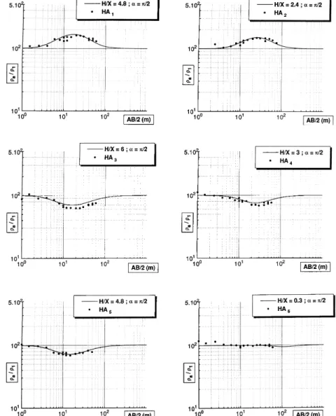
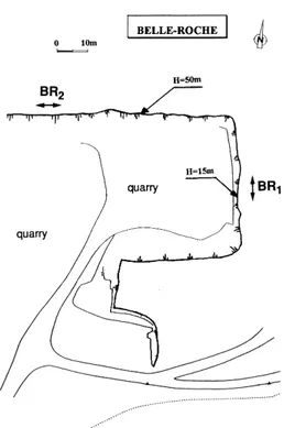
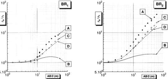
(10) 804. H. Sahbi, D. Jongmans and R. Charlier. Figure 7. Location of the Schlumberger soundings (HA1 to HA6) at the Hallembaye site. (a): Map view; (b): cross-section along the line I-II.. with other models, including three-layer cases with different resistivity conditions. For all the models tested, the difference between the results after correction and the 1D theoretical curve is less than 2%.. Field example The correction procedure has been tested in a limestone quarry (Belle-Roche) during resistivity measurements. Several Schlumberger tests were conducted parallel to an old exploitation face whose height varies between 15 m and 50 m (Fig. 10). The solid rock is overlain by a weathered layer and by a clay overburden a few metres thick. The first electric sounding (BR1) was performed on a surface where the overburden was removed, while the second one (BR2) was located on the natural ground. The two soundings were located at 4 m (BR1 ) and 2.5 m (BR 2 ) from the cliff. The measured apparent resistivity values for the two soundings are drawn on Fig. 11. The curves are normalized with the resistivity in the clay layer (45 Qm). In a bilog diagram, the slope of the two experimental curves (A) for a spacing over 10 m is higher than 458, which makes any fitting with a horizontally layered model impossible. This is clearly a topographic effect, which has been removed by numerical modelling. The correction curves (B) and the corrected apparent resistivity values (C) are shown in the same figure. In both cases, the correction effect is to decrease the resistivity values and to reduce the slope angle. For BR1, a striking feature is that the initial curve (A) shows a slope variation at AB/2 ¼ 30 m, which corresponds to the maximum of the correction curve (B) and. q 1997 European Association of Geoscientists & Engineers, Geophysical Prospecting, 45, 795–808.
(11) Slope effects in resistivity surveys 805. Figure 8. Comparison between the experimental data (Hallembaye site) and the simulation results in a nondimensional graph. The vertical scale of the normalized apparent resistivity has been enhanced.. which has disappeared on the final curve (C). Within a layered model, the interpretation of curve (C) gives a weathered limestone layer with a resistivity of 1250 Qm and a thickness of 7 m, overlying a limestone bedrock characterized by a resistivity of 10 000 Qm. The small resistivity decrease observed on curve (C) for AB/2 around 8 m is thought to be a 3D effect generated by the presence of a clay pocket.. q 1997 European Association of Geoscientists & Engineers, Geophysical Prospecting, 45, 795–808.
(12) 806. H. Sahbi, D. Jongmans and R. Charlier. Figure 9. Theoretical topographic effect of a cliff (H ¼ 100 m) in a two-layer medium. The surficial layer thickness T is 10 m. The vertical scale of the apparent resistivity has been slightly enhanced. Left: the resistivity of the surficial layer (r1 ¼ 1Qm) is lower than that of the deep layer ( r2 ¼ 10 Qm). Right: the resistivity of the surficial layer (r1 ¼ 10 Qm) is higher than that of the deep layer ( r2 ¼ 1Qm). A: apparent resistivity curve in a two-layer ground with a cliff; B: apparent resistivity curve in a homogeneous ground with a cliff; C: apparent resistivity curve in a flat two-layer ground.. Figure 10. Location of the Schlumberger soundings (BR1 and BR 2 ) at the Belle-Roche site.. q 1997 European Association of Geoscientists & Engineers, Geophysical Prospecting, 45, 795–808.
(13) Slope effects in resistivity surveys 807. Figure 11. Apparent resistivity curves measured at the Belle-Roche site (BR1 and BR2) and simulation results. A: experimental apparent resistivity curves; B: correction curves; C: apparent resistivity curves corrected for the topographic effect; D: 1D interpretation.. After correction, the sounding BR2 has pointed out a three-layer structure consisting of a 3 m thick clayey overburden (40 Qm) overlying 5.5 m of weathered limestone (1250 Qm) and the unweathered bedrock (10 000 Qm). Without correction, it would have been impossible to get good agreement between experimental data and a three-layer model curve.. Conclusions A 3D computer algorithm has been used for simulating the topographical effect in the case of a 2D slope, when Schlumberger soundings are parallel to the strike. The slope is defined by its angle and height. The results are presented as nondimensional curves (Figs 2 and 3) which can be used for evaluating terrain effects in any configuration. Using the method initially proposed by Fox et al. (1980), we showed on synthetic cases that the topographic effect can be correctly removed from Schlumberger sounding data. In order to test our theoretical results, field experiments were performed in different geological conditions including a tailing heap and quarries. In homogeneous ground, the validity of the theoretical nondimensional curves has been confirmed by the field data. In a layered medium, the measured resistivity curves appeared to be significantly disturbed by topographic effects and 1D interpretation may clearly lead to erroneous results, even with electrode arrays parallel to the strike. Using the nondimensional diagrams, these curves have been successfully corrected to obtain the layered ground characteristics.. q 1997 European Association of Geoscientists & Engineers, Geophysical Prospecting, 45, 795–808.
(14) 808. H. Sahbi, D. Jongmans and R. Charlier. References Cecchini A. and Rocroi J.P. 1980. Effet topographique en prospection e´lectrique. Geophysical Prospecting 28, 977–993. Coggon J.H. 1971. Electromagnetic and electrical modelling by the finite element method. Geophysics 36, 132–156. Dey A. and Morrison H.F. 1979a. Resistivity modelling for arbitrarily shaped two-dimensional structures. Geophysical Prospecting 27, 106–136. Dey A. and Morrison H.F. 1979b. Resistivity modelling for arbitrarily shaped threedimensional structures. Geophysics 44, 753–780. Fox R.C., Hohmann G.W., Killpack T.J. and Rijo L. 1980. Topographic effects in resistivity and induced-polarization surveys. Geophysics 45, 75–93. Hedstro¨m H. 1932. Electrical prospecting for auriferous quartz veins and reefs. Mining Magazine 46, 201–213. Holcombe H.T. and Jiracek G.R. 1984. Three dimensional terrain corrections in resistivity surveys. Geophysics 49, 439–452. Koefoed O. 1976. Progress in the direct interpretation of resistivity sounding: An algorithm. Geophysical Prospecting 24, 233–240. ¨ . 1954. Mapping nearly vertical discontinuities by earth resistivities. Geophysics 19, 739– Logn O 760. Molano C.E., Salamanca M. and Van Overmeeren R.A. 1990. Numerical modelling of standard and continuous vertical electrical soundings. Geophysical Prospecting 38, 705–718. Pridmore D.F., Hohmann G.W., Ward S.H. and Sill W.R. 1981. An investigation for finiteelement modelling for electrical and electromagnetic data in three dimensions. Geophysics 46, 1009–1024. Queralt P., Pous J. and Marcuello A. 1991. 2-D resistivity modelling: an approach to arrays parallel to the strike direction. Geophysics 49, 439–452. Telford W.M., Geldart L.P. and Sheriff R.E. 1990. Applied Geophysics, 2nd edn. Cambridge University Press. Zienkiewicz O.C. 1989. The Finite Element Method, 4th edn. McGraw¹Hill Book Co.. q 1997 European Association of Geoscientists & Engineers, Geophysical Prospecting, 45, 795–808.
(15)
Figure
Documents relatifs
Influence of sliding interfaces on the response of a layered viscoelastic medium under a moving load
Mechanical response under a moving load of a viscoelastic four-layer structure with a bonded or a slip boundary between layers 2 and 3: influence of the velocity on the normal
The effect of particle shape and orientation on the effective resistivity of a heterogeneous medium was simulated for laboratory or field measurements, as shown in Figure
Rate coefficients for temperatures ranging from 5 to 150 K were computed for all hyperfine transitions among the first 15 rotational energy levels of both ortho- and para-NH 2
The final filter design uses a geneva drive to index wheels containing pairs of high-pass and low-pass filters into the light path between the light source and the test specimen..
These studies demonstrated that the increase of the specific surface area (higher silanol concentration 12 ) and pore volume of bioactive glasses has an effect
On the other hand, one of the most fascinating properties of spin glasses, which makes this state of matter a very peculiar one, is the onset of remanence effects for very weak
The first step was to calculate, using the density functional formalism [10, 11], the displaced electron densities around a nucleus embedded in a jellium vacancy for
But, in this case, in the institutionalization phase the teacher could have used the students’ explanation of their strategy and the fact that students mention that
