par
Guennadi Chitov
These presentee au departement de Physique en vue de 1'obtention du grade de Docteur es sciences (Ph.D.)
FACULTE DES SCIENCES
UNIVERSITE DE SHERBROOKE
Sherbrooke, Quebec, Janvier 1998
//
o?
^
'V, ^5^//^
/"? /-/ r-i!Js'r'^//'-^
THE FERMI LIQUID AS
A RENORMALIZATION
GROUP FIXED POINT
1*1
of Canada Acquisitions and Bibliographic Services 395 Wellington Street Ottawa ON K1AON4 Canada du Canada Acquisitions et services bibliographiques 395, rue Wellington Ottawa ON K1AON4 CanadaYour file Votre reference
Our file Notre reference
The author has granted a
non-exclusive licence allowing the
National Library of Canada to
reproduce, loan, distribute or sell
copies of this thesis in microform,
paper or electronic formats.
The author retains ownership of the
copyright m this thesis. Neither the
thesis nor substantial extracts from it
may be printed or otherwise
reproduced without the author's
permission.
L'auteur a accorde une licence non
exclusive pennettant a la
Bibliotheque nationale du Canada de
reproduire, preter, distribuer ou
vendre des copies de cette these sous
la forme de microfiche/fihn, de
reproduction sur papier ou sur format
electronique.
L'auteur conserve la propriete du
droit d'auteur qui protege cette these.
Ni la these ni des extraits substantiels
de celle-ci ne doivent etre imprimes
ou autrement reproduits sans son
autonsation.
0-612-35763-5
Le -2'^ | ^ I ^ _ , Ie jury suivant a accepte cette these dans sa version finale.
date
President-rapporteur: M. Claude Bourbonnais Departement de physique
Membre: M. David Senechal
Departement de physique
Membre: M. Andre-Marie Tremblay
^-- ^
Departement de physique
Membre externe: M. Victor Yakovenko I/ ^ OVVY lvl . Universite de Maryland
The renormalization-group (RG) method is applied to study interacting fermions at finite temperature. A model based on the '04-Grassmann effective action with 5'[/(A^)-invariant short-range interaction and a rotationally invariant Fermi surface in spatial dimensions d = 2,3 is studied. We show how the key results of the Landau Fermi liquid theory can be recovered by this finite-temperature RG technique. Applying the RG to response functions, we find the compressibility and the spin susceptibility as solutions of the RG flow
equations.
We discuss subtleties associated with the symmetry properties of the four-point vertex (the implications of the Pauli principle). We point out distinctions between three quantities: the bare interaction of the low-energy effective action, the Landau function and the forward scattering vertex. The bare interaction of the effective action is not a RG fixed point, but a common starting point of the flow trajectories of two limiting forms of the four-point vertex. We have derived RG equations for the Landau channel that take
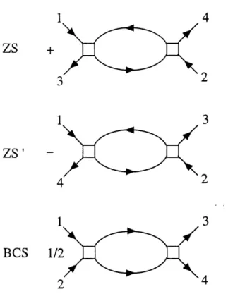
into account both contributions of the direct (ZS) and the exchange (ZS )
particle-hole graphs at one-loop level. The basic quantities of Fermi Liquid theory, the Landau interaction function and the forward scattering vertex, are calculated as fixed points of these flows in terms of the effective action's interaction function.
The classic derivations of Fermi Liquid theory applying the Bethe-Salpeter equation and other analogous approaches, tantamount to some sort of RPA-type (decoupled) approximation, neglect the zero-angle singularity in the ZS' graph. As a consequence, the antisymmetry of the forward scattering vertex is not guaranteed in the final result, and the RPA sum rule must be imposed by hand on the components of the Landau function to satisfy the Pauli principle. This sum rule, not indispensable in the original phenomenological formulation of the Landau FLT, is equivalent, from the RG point of view, to a fine tuning of the effective interaction.
Our results show that the strong interference of the direct and exchange processes of the particle-hole scattering near zero angle invalidates the R.PA
(decoupled) approximation in this region, resulting in temperature-dependent narrow-angle anomalies in the Landau function and scattering vertex, revealed by the RG analysis. In the present RG approach the Pauli principle is automatically satisfied. As follows from the RG solution, the amplitude sum rule, being an artefact of the RPA approximation, is not needed to respect statistics and, moreover, is not valid.
I would like to thank cordially my adviser and collaborator David Senechal for continuous support, gentle guidance and innumerable enlightening discussions. It was a great pleasure for me to work with him. I particularly appreciate his patience in editing all my "literature activities" in English.
I thank very much Andre-Marie Tremblay for many stimulating discussions, continuous interest in my work, and for careful and critical reading of my
manuscripts.
I thank Nicolas Dupuis, my collaborator in part of this work and a very interesting interlocutor with whom I discussed many subtle questions in the
course of my work.
I express my gratitude to Claude Bourbonnais and Yury Vilk for many helpful conversations and sharing their knowledge on subjects I have been trying to learn more about.
I would like to thank the Departement de Physique and the Centre de Recherche en Physique du Solide (C.R.P.S.) for their hospitality and for giving me a chance to carry out my work in an atmosphere of friendship and scientific devotion, created by people working there. I particularly acknowledge the financial support from C.R.P.S. during all my stay in Sherbrooke.
TABLE OF CONTENTS
SUMMARY ... ii
ACKNOWLEDGEMENTS. ... iv
TABLE OF CONTENTS ... v
LIST OF FIGURES ... vii
CHAPTER 1: Introduction ... 1
CHAPTER 2: RG Preliminaries ... 13
2.1 The RG method ... 13
2.2 The model ... 22
2.3 Tree-level RG analysis ... 29
2.4 Coupling functions and vertices ... 34
CHAPTER 3: RG without interference ... 40
3.1 The Landau channel ... 40
3.2 RG equations in the BCS channel ... 48
3.3 RG equations in three dimensions ... 50
3.4 Response functions ... 54
CHAPTER 4: Role of the interference in the Landau channel ... 58
4.1 Coupled RG equations in the Landau channel ... 58
4.2 Deficiencies of the decoupled approximations in the Landau channel 63 4.3 Solution of the coupled RG equations ... 66
4.3.1 Exact numerical solution ... 66
4.4 Analysis and discussion of the RG results ... 72
4.5 Contact with the Landau FLT and discussion ... 76
Conclusion ... 82
LIST OF FIGURES
1. The three diagrams contributing to the RG flow at one-loop ... 41
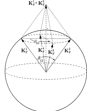
2. Conic momentum configuration in the 3D case ... 50
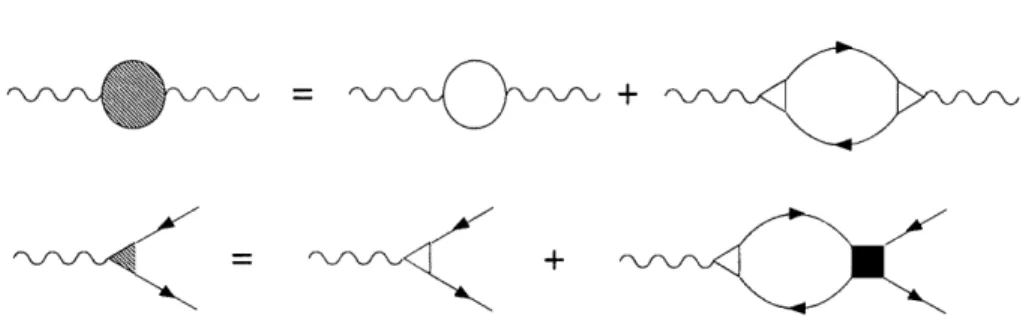
3. Diagrams for the calculation of response functions ... 57
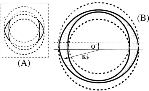
4. Phase space constraints ... 60
5. Numerical solution of the R,G equations. ... 73
CHAPTER I
Introduction
In 1956-1957 L.D. Landau formulated his theory of Fermi liquids.1 Let us first recall briefly the crucial premises of Landau's phenomenology It is assumed that the ground state of the interacting fermion system at T = 0 is in one-to-one correspondence with that of the ideal Fermi gas, i.e., the Fermi sea is filled up to the Fermi momentum kp, which is related to the fermion density in the same fashion as for non-interacting fermions (d = 3):
^=2/no(k)^=^. (1.1)
Here N is the number of fermions and V is the volume of the system. We will set from now on kp = h = 1. The ground-state distribution function no W at T = 0 is just the Heaviside step function:
no(k) =Q(kF-k) . (1.2)
The excitations of this system are created when particles from the filled Fermi sphere pass to the available states with k > kp- Landau's idea was to describe the low-lying excitations in the interacting system (i.e., the excitations into the states with k such that \k — kp\ <^ kp) in terms of fermion quasiparticles which have a spectrum like that of free particles, but renormalized because of interactions. The invariance of the Fermi sphere's volume under switching on the interaction, expressed by Eq. (1.1), can be interpreted as the following statement: the number of quasiparticles equals the number of real fermions constituting the system, i.e., Nqp = N. Notice that the total energy of the interacting fermion system (the Fermi Liquid) is not an additive quantity of the quasiparticle energies e(k), contrary to the ideal Fermi gas
E _ f /_ /_ d3k
£=^2yn(k)e(k).
'w '
Instead, Landau proposed the following expansion for the total energy
£[<^(k)]=£o+ />£o(k)<5n(k)+^ / /(k,k')(5n(k)($n(k/) (1.3)
in terms of the variations 6n of the quasiparticle's distribution function n(k) over the ground-state distribution no (k)
6n(k) = n(k) - no(k) . (1.4)
£o stands for the ground-state energy at zero temperature and the following
short-hand notations are used:
d3k
L =J (^ • (L5)
Unless necessary, we will not write down explicitly the spin dependence of the parameters, indicating it by hats only, e.g., n(k) ^-> na^(k), -etc. The energy of the quasiparticle is given by
e(k) = ^ = eo(k) + j f(k, k')5n(k') , (1.6)
wherein £o(k) gives the equilibrium energy of the quasiparticle at zero temperature. The /-function, accounting for the interactions between quasiparticles in the Fermi Liquid (the Landau interaction function), is defined as follows:
/(k,k')=^^^^ . (1.7)
mfk/'Being the second derivative of the energy, which is invariant under the exchange <!m(k) <-^ ((m(k ), the Landau function satisfies the symmetry properties
/^(k,k/)=/^(k/,k) . (1.8)
The Landau picture of quasiparticles is limited to the close vicinity of the Fermi sphere when the quasiparticle's momenta satisfy the condition \k — kp\ <€ kp, and to the low temperatures T <; Ep^ when the equilibrium quasiparticle's distribution function differs from the step function (1.2) only in a narrow neighborhood of width T around the Fermi energy. Then the quasiparticle energy £o(k), measured from the zero-temperature value of the chemical potential p,(T = 0) = Ep = A^/2m*, can be written as £o(lc) ^ ^(k — kp) wherein m* is the quasiparticle effective mass. The quasiparticle at low temperature is a well-defined excitation, since its life-time r
increases as r oc T when T —> 0. Since <5n(k) is appreciable only in the immediate proximity of the Fermi surface, the quasiparticle momenta k and k/ entering the Landau function / can be put at the Fermi surface, so / will depend on the directions of those vectors only. If the system is spin-rotationally invariant (e.g., there is no external magnetic field), the Landau function simplified in such manner depends only on the relative angle 6 between the vectors k and k , where |k| = |k | = kp- In such case the Landau function can be represented by two dimensionless angular functions F and G as follows:
^F • /a/3,75(k, k/) = Vp • fa(3,^sW = ^(0)8^6^ + G(0)cr^ • 0-^5 , (1.9) wherein vp ls ^he density of electron states on the Fermi .level and cr are the Pauli matrices. It is convenient to use the coefficients {Fi,Gi} of the Legendre
polynomial expansion of {F(0),G(6)} (cf. definition of this expansion (3.39)
below). To emphasize the significance of the Landau function, characterizing quantitatively the Fermi Liquid state, we recall some exact results of the Fermi Liquid Theory (FLT). The components of the /-function enter into formulas for the physical observables, resulting in a renormalization of the free Fermi gas results, due to the interaction effects. The interaction coefficient F\ provides the exact relationship between the quasiparticle effective mass and the (bare) mass of the real interacting particles:
^-=l+Fl . (1.10)
m
The above relationship is exact since it follows from Galilean invariance. In turn, the renormalized effective mass enters the Fermi-gas-type linear temperature dependence of the specific heat C = ^m^kpT. The interaction effects in the Fermi Liquid result in renormalization factors (1 4- -Fo) and
(1 + Go) in the Fermi-gas formulas for the compressibility (K) and the spin
susceptibility (x)i respectively:
1 ~U-p 1 2 1<F
1 A. — 7J
n21 +FQ ' ^ - 4y 1 + C?o '
wherein n is the particle density and g is the gyromagnetic ratio. For the thermodynamic stability of the energy functional (1.3) Pomerandiuk derived the conditions for the components of the Landau interaction function:2
Shortly after the appearance of the Fermi Liquid phenomenology, much effort has been dedicated, including by Landau himself, to vindicate some intuitive assumptions of Landau and elucidate the foundations of the phenomenological theory. The original phenomenological formulation of this theory is formulated in terms of bosonic variables [variations of the distribution function n(k)]. The field-theoretic interpretation of the Landau FLT has reformulated the key notions and basic results of the phenomenological theory entirely in terms of the fermionic Green functions technique. 3'4'5'6 The demonstration of the equivalence of the field-theoretic results obtained from the solution of the Bethe-Salpeter equation with the results obtained from the functional expansion (1.3) and from the Boltzmann transport equation describing the collective modes, has become a textbook topic. 5'6'7'8'9 The field-theoretic approach provided not only a solid basis to phenomenology but also a potentially efficient method to calculate the phenomenological parameters of FLT from first principles. Silin's extension of the FLT, which incorporates the long-range Coulomb interaction between particles, made this theory applicable to charged Fermi liquids as well.10
The conditions under which the FLT breaks down have also been well known for a long time. If the Pomerandiuk stability conditions (1.11) or the Landau theorem for the stability of Fermi Liquid against Cooper pairing at arbitrary angular momentum are not satisfied, then a phase transition towards a phase different from the Fermi Liquid could occur. (This theorem demands, roughly speaking, the absence of effective attraction for all components of the interaction function. For the exact conditions of this theorem see Eqs (3.27) below.) For instance, the attraction between fermions violates the conditions of Landau's theorem, and the superconductive phase transition takes place. Another classical example is provided by interacting fermions in one spatial dimension, wherein the FLT never works, even without spontaneously broken symmetry (phase transition). Instead, the operational notion in ID is what was called by Haldane the Luttinger Liquid.11 (For a recent review on ID systems see, e.g., the paper by Voit.12) However, the discovery of the fractional quantum Hall effect13'14 and of high-Tc super conductors15 revealed the existence in Nature of completely new phases of fermion systems in d > 1 with unbroken
symmetry, which do not fit in the description provided by the FLT. Those two extraordinary discoveries engendered a new branch of condensed matter physics, the physics of strongly correlated fermion systems. For reviews on the recent developments in this rapidly advancing field see, for example, Refs. 16,17] and more references therein.]
Current interest in the physics of strongly correlated fermions [non-Fermi
Liquids in d > 1] inspired a new wave of efforts aimed at clarifying the
foundations of the Landau FLT and possible mechanisms of its breakdown. Let us mention only two approaches, which can be seen as sophisticated modern counterparts of the two classic formulations of the Landau FLT. Developing Luther's earlier ideas,18 Haldane put forward the method of higher-dimensional bosonization19 in order to treat the Fermi Liquid. Followed by other studies, bosonization approaches to various fermionic liquids have recently been developed.20'21'22'23 At about the same time, the Renormalization Group (RG) technique has been applied to interacting fermions in d > 1 with models based on fermionic field effective actions (see Refs. [24-34] and references therein). In both approaches it has been established, for models with reasonable fermion-fermion effective interactions, that the Fermi liquid phase is stable, whereas adding gauge-field interactions may drive the system towards a Non-Fermi-Liquid regime, or may result in a Marginal Fermi Liquid phase, like for composite fermions at the half-filled Landau level.
This work is devoted to the development of the RG approach to interacting fermions. However, we feel obliged to mention our reservations about the first method mentioned above, namely, bosonization in d > 1. Our concerns are, basically, two-fold. Firstly, for the simplest case of the effective action for short-range interacting fermions, the higher-dimensional bosonization approach allowed to recover most of the known results of Landau's phenomenology But this method does not give even a conceptual clue as to what the parameters of the Fermi Liquid should be (i.e., do the coefficients of the Landau function satisfy the Pomerandiuk stability conditions?) and how they can be traced over from a microscopic Hamiltonian. Secondly, in cases of more complicated effective
actions which include, e.g., additional gauge and/or other fields and which are less well understood, the results provided by the bosonization may be controversial, since the simplifications done in order to get the approximated (Kac-Moody) algebra for the boson variables are hard to control. For instance, the authors of Ref. [36], who applied field-theoretic methods to treat interacting fermions coupled to a gauge field, claim that the bosonization results20 for that problem are valid only in the unphysical limit N —> 0, wherein N is the number of fermion species. For a more detailed discussion of the generic bosonization algebra, its approximations and related issues, see, e.g., Ref. [22].
Until recently, the most successful applications of RG methods to interacting fermions have been achieved in the one-dimensional case, where it was known from exact solutions that non FL phases exist (e.g., the Luttinger liquid). For earlier reviews on ID systems see Refs. [37,38]. Later, Bourbonnais and Caron made an extensive RG study of one-dimensional and quasi-one-dimensional fermion systems at finite temperature. The necessity for theorists to understand the occurence of Non-Fermi-Liquid phases (or regimes) of interacting fermions in "isotropic"^ systems of dimensions greater than one, explains naturally the interest in the development of a RG theory for such systems. The RG is known to be a powerful method, well-established in other fields of physics,40'41'42'43 systematic in the sense of a control over approximations done in practical calculations, and capable of giving results far beyond the reach of perturbational approaches. As discussed by Shankar in a very pedagogical paper,28 the RG treatment of fermions in the context of condensed matter problems is a much more complicated issue than the analogous procedure for critical phenomena or quantum field theories, because of two crucial points: Firstly, the existence of a Fermi surface: the low-energy modes lie in the vicinity of a continuous geometrical object (the Fermi surface) and not only around isolated points, like the origin of phase space in the bosonic case. Technically, this introduces additional phase space constraints on ^ In the sense that the system cannot be treated as a set of weakly coupled one-dimensional chains.
the modes to be integrated out, quite a problem for an arbitrary Fermi surface. Moreover, the Fermi surface itself is a relevant parameter of theory, and its shape should renormalize under the RG procedure, except in the rotationally symmetric case. Secondly, instead of studying the flow of one or a few coupling constants like in other familiar physical problems, one has to treat RG flow equations for coupling functions, defined on the Fermi surface. Notice that the purely ID interacting fermion system can be considered as a degenerate special case where the Fermi surface is reduced to a set of two points, with a finite number of coupling constants. It is therefore closer to the usual applications of the renormalization group. (However, in the quasi-one-dimensional approach of Ref. [39], one already witnesses the appearance of new coupling constants related to interchain hopping and one may follow the change in shape of the
(open) Fermi surface under RG flow.)
Let us now more specifically discuss the RG studies of the Fermi Liquid phase. It will allow us to place our results in the context of other workers's contributions to the field, and to explain the motivation and goals of our work.
The RG studies of interacting fermions cited above24'25'27'28'29'30 contain general statements on the stability of the Fermi Liquid phase in d = 2,3 in the case of short-range repulsion. However, the standard formulas and relationships of the Landau FLT were not recovered in those papers. To the best of our knowledge, only in the paper of Shankar were those questions addressed28 and he was closer than others to the right treatment of the FLT from the RG standpoint. Shankar correctly treated the Bardeen-Cooper-SchriefFer (BCS) interaction channel of scattering quasiparticles with opposite incoming (outgoing) momenta and recovered the Landau theorem for the stability of the Fermi Liquid against Cooper pairing. Treating then the Landau interaction channel of nearly forward scattering quasiparticles, Shankar recovered some of the FLT results, combining the tree-level RG analysis with perturbation theory. He also tried to clarify the relationship between the parameters of the interaction appearing in the fermionic effective action and the Landau interaction function of the conventional FLT. Nonetheless, working at zero
temperature, Shankar erroneously concluded that there is no RG flow of the coupling functions (vertices) in the Landau interaction channel. (We will show below that working in the framework of the finite-temperature RG technique allows us to find results for the Landau channel that were missed by Shankar. The reason is that the /3- function (i.e., the r.h.s. of the RG flow equation) for the running couplings in that channel becomes singular at T = 0, and it is easy to get the wrong result in the zero-temperature limit.) As a consequence, Shankar was not able to distinguish between the forward scattering amplitudes (scattering vertex) and the Landau interaction function, known from the field-theoretic version of the FLT to be two different zero-transfer limits of the non-analytic four-point vertex.5'6'7 Notice that the mistake of neglecting the RG flow for the forward scattering vertex was partially circumvented in Shankar's paper by applying perturbation theory (or, more exactly, by summing an infinite series of particle-hole ladder diagrams) for the calculation of the physical observables involving that vertex, e.g., the compressibility. Eventually it gave the standard RPA-type result which could have been directly provided by the RG at the one (particle-hole) loop level. 3 However, Shankar's neglect of the RG flow in the Landau channel also resulted in another problem, since by
doing so he mistakenly identified the (bare) coupling function of the effective
interaction with the Landau interaction function. Indeed, the latter has to be identified with a fixed point of the RG equations, but when the corresponding RG flow given by the /3-function of those equations is found to be identically zero (Shankar's case), then the bare value (initial point of the flow) and the fixed-point value of the coupling function are the same.
Let us give two arguments showing, even without explicit calculation of the RG flow equation whose solution gives the Landau interaction function, why this flow is non-zero and, consequently, why the bare interaction function of the low-energy fermion effective action cannot be identified with the Landau interaction function. First, identifying the Landau function with the effective action's bare interaction is inconsistent with other standard FLT results, because of the role of Fermi statistics (the Pauli principle). Let us consider for simplicity two-dimensional spinless fermions. Then the Landau interaction
function defined as in Eq. (1.9) is totally determined by a single function F(0)
or, equivalently, by the set of its Fourier components FI. The forward scattering vertex constructed and decomposed in the same fashion as the /-function in Eq. (1.9), is given for the case in hand by a single "charge" component, which we will denote T(0). The Pauli principle for the scattering vertex demands that T(0 = 0) = 0. Then the statement is that in a stable Fermi liquid, the standard relationship between Fourier components of the scattering amplitude (fi) and of the Landau interaction function (Fi), i.e., TI = FI/(I + -^), cannot satisfy the
Pauli principle for the amplitude (the amplitude sum rule)
Ft
ST
-1+F,
=0 (1.12)
if F has the symmetry properties of the action's bare interaction i.e., if
F{0 = 0) = ^ ^ = 0. (For the explanation and rigorous proof of this point
see Sec. 4.2 below). Second, identifying the Landau function with the bare interaction is inconsistent with the premise of low-energy effective action method itself, in the way it is applied to condensed matter problems. Namely, at the starting point of the analysis, the bare parameters of the effective action, including the interaction, are regular functions of their variables.27'28 It is known, however, that this is not the case even for parameters of a normal Fermi liquid. The scattering amplitude and the Landau function are two distinct limits of the four-point vertex when energy-momenfcum transfer goes to zero. This non-analyticity of the vertex appears in its dependence both on the small energy-momenfcum transfer and, due to the crossing symmetry, on the small angles between incoming (outgoing) particles lying near the Fermi surface. This contradiction between the analytical properties of the two functions in question (i.e., the bare interaction and the Landau function) becomes flagrant in the case of more exotic fermion systems. For instance, the Landau function of the marginal Fermi Liquid of composite fermions at the half-filled Landau level (interacting fermions coupled with gauge field) is shown by other (non-RG) methods44 to develop a ^-function singularity in the forward direction (6=0). Such behavior of the Landau function is related to the divergence of the quasiparticle's effective mass, according to the theory of
Halperin, Lee and Read for the half-filled Landau level45 (see also Ref. [46]).
So, our two arguments show that the Landau function cannot be a regular interaction in the effective action at the starting point of the RG analysis.
The preceding comments on the earlier RG approaches to Fermi Liquids show that they are insufficienfc on many points. Let us now give a general outlook of the key components of our study which presents the quantitative RG theory of the Fermi-Liquid fixed point.
The first part of our RG results for the FLT, presented in Chapter 3, like other such analyses already published, are obtained from a low-energy effective action27'28'29 with a marginal (in the RG sense) short-range interaction at the starting point of the RG procedure. However, contrary to other works on the subject, our finite-temperature RG approach reveals that, in the Landau channel of nearly forward scattering quasiparticles, the effective action's coupling functions flow with successive mode eliminations towards the Fermi surface, even in the absence of singular or gauge interactions. In other words, the coupling functions do not stay purely marginal under the RG transformation, since their /5-functions are not identically zero. From the RG flow equations which explicitly take into account the direct particle-hole loop (ZS) only^ the standard FLT formulas for the susceptibilities and the relationships between the scattering amplitudes and the components of the Landau function are recovered. The formulas of the conventional FLT, obtained at that stage of the study, are strictly equivalent to the results of the classic diagrammatic approach to Fermi Liquid.
The aim of the next stage, presented in Chapter 4, is twofold. Once the classic FLT results have been recovered by the RG approach in the form of relationships between fixed-point values of different coupling functions (running vertices), the approach itself would loose its appeal if it did not provide a constructiw method for calculating the Fermi liquid s parameters. This is especially important goal in the long-term perspective of applying this powerful method to more complex (strongly correlated) fermion systems. In order to
provide that kind of quantitative RG theory, we explicitly calculate the Landau function and the forward scattering vertex, starting from the short-range effective bare interaction. We do it in a one-loop RG approximation which takes into account contributions of the direct (ZS) and exchange (ZS) particle-hole graphs. In particular, this enables us to reveal singular temperature-dependent features of the Landau function and scattering vertex in the forward direction
(e = o).
An equally important goal of that second part of the RG analysis is to resolve the old problem of FLT with the Pauli principle. In its treatment of FLT, the field-theoretic approach encountered a very subtle problem caused by Fermi statistics and by the necessity to provide both stability for the Fermi liquid and a solution for the two-particle vertex (scattering amplitude) that meets the Pauli principle.47'7 (We remind, that according to the requiremenfcs of Fermi statistics, the two-particle vertex is antisymmetric under exchange of the incoming (outgoing) particles.) The problem was "settled" by imposing (practically by hand) the amplitude sum rule on the components of the Landau quasiparticle's interaction function. [Cf. the example of such sum rule for the case of fermions without spin given above by Eq. (1.12).] It is worth noting that the phenomenological FLT is spared from this problem partially because it is formulated in terms of bosonic variables see, e.g., Eqs. (1.3-1.7)], partially because it says nothing about the two-(quasi)particle fermion vertex. Landau's phenomenology only provides us with the condition (1.8) for the symmetry properties of the /-function. As we can easily see from Eq. (1.9), in the absence
of SU(2) symmetry breaking fields (interactions) any function of the relative
angle between quasiparticle momenta meets the requirement; (1.8). In the phenomenological theory no more constraints (sum rules) on the functions F, G are implied. Seen from the RG standpoint, the same problem of constraints manifests itself in the form of a "naturalness problem"2 of the effective action: the low-energy effective action has to be fine tuned" in order for the scattering amplitude to meet the Pauli principle. More detailed discussion of this problem is postponed until Sec. 4.2, where it will be put in contact with the present RG approach. It will be shown in Chapter 4 that if quantum
interference of the direct and exchange processes is taken into account in the RG equations, this problem is eliminated in a natural manner.
The' thesis is organized as follows. In Chapter 2 we give a short description of the RG method, we define the model to be studied and the quantities to be calculated by the present RG technique. In Chapter 3 we develop the (decoupled) one-loop RG approach to the model based on the fermionic low-energy effective action. We demonstrate that such an approach is equivalent to the classic field-theoretic treatment of the Fermi liquid. In Chapter 4 we derive and solve the RG equations which explicitly preserve the exchange symmetry of the four-point vertex. From a more physical point of view, the novelty of those equations is the handling of the interference between the direct and exchange particle-hole processes in the Landau channel of the (nearly) forward scattering particles. The consequences of the RG corrections on FLT
results are discussed.
In the beginning of each chapter we give a short description of its content. The main results of this thesis have been presented in Refs. [33,34,35]
CHAPTER II
RG Preliminaries
This chapter is mostly introductory. It contains auxiliary information and the results of a scaling analysis, necessary in order to venture beyond tree-level in the RG calculations. In Sec. 2.1 we give a short summary of the RG method. In Sections 2.2 we define the effective action of the model. At the technical level, the model is a straightforward extension of that considered earlier by Shankar for spinless fermions at zero temperature. The extension incorporates spin and a finite temperature. For the sake of generality, we study a model of A^-component fermions with an SU{N)-mva,na,Tit short-range interaction. We study the effective action defined for a circular Fermi surface in spatial dimension two, spherical in dimension three. The scaling analysis of Sec. 2.3 allows us to single out two interaction channels (Landau and BCS) wherein the coupling functions of the effective action s interaction are marginal at tree level. The Landau interaction channel corresponds to the (nearly) forward scattering processes of (quasi)particles in the vicinity of the Fermi surface. The Bardeen-Cooper-SchriefFer (BCS) interactions channel corresponds to the scattering of the (quasi) particles with opposite incoming (outgoing) momenta near the Fermi surface. In Sec. 2.4 we define the coupling functions (running vertices) to be calculated in the RG framework in both channels.
2.1 The RG method
In many fundamental domains of physics it is necessary to handle a problem of interacting (coupled) fields, i.e., a problem containing a very large number of interacting degrees of freedom (infinite in the continuum limit). This is the usual situation in Quantum Field Physics and in Condensed Matter Physics. What particularly complicates the analysis in most cases is that interactions between fields cannot be considered as weak, nor can a problem be satisfactorily solved by singling out some characteristic mode from the ensemble
of interacting fields. The latter means that if, say, we have fields (p(k) wherein k is wavenumber, then we cannot obtain a good approximation by separately treating a single degree of freedom y?(/co) specified by the wavenumber ko. The scale ko can be usually chosen on physical grounds. In many situations such kind of treatment, which is tantamount to some sort of mean-field approximation, fails.
Unfortunately, there are only very few physically interesting exactly solvable models in field theory or statistical physics and, moreover, their exact solutions can be found only in low spatial dimensions48'49 (Examples of such exactly solvable problems are provided by the Tomonaga-Luttinger model of interacting fermions in d = 1, the Ising model in d =1,2.) However oversimplified those models might appear, much can be learned from their solutions. The complexity of the problem with interacting fields, classical or quantum, which precludes the use of a naive perturbation calculation around the non-interacting or mean-field solution, is due not only to - and in some cases not necessarily to - the strength of interactions, but also to the large number of degrees of freedom involved in the relevant physics and correlations between them. For instance, for ID fermions, it is known that any interaction, however weak, destroys the Fermi liquid phase. The latter is the mean-field approximation for interacting fermions. Prom a technical point of view, the absence of a single momentum (energy) scale and, instead, the involvement of a, continuum of modes below some characteristic scale (~ Ep)^ is signalled in perturbation (diagrammatic) calculations by appearance of the logarithmically
divergent terms (a \TI(EF/E), E -> 0).
The problem of phase transitions provides another well-known example of physics essentially involving a continuum of degrees of freedom. For the sake of simplicity, let us consider the transition at the Curie temperature (Tc) from a paramagnetic state to a uniaxial ferromagnet. This type of transition can be described by studying a one-component classical fluctuating field ^p(k). It is known that the Landau mean-field theory, which is formulated in terms of the average of this field only (i.e., the magnetization m = (y?(0)) for the
example chosen), gives wrong predictions for the temperature behavior of thermodynamic parameters (e.g., magnetization, specific heat, susceptibility) near Tc in spatial dimensions d <: 3. In the parlance of the theory of critical phenomena, the mean-field theory predicts wrong values of critical exponents in d ^ 3. (For reviews on this subject see, e.g., Ref. [40,50], as well as Ref. [51] for the original pedagogical formulation of Landau's theory of phase transitions. Interestingly enough, the non-mean-field critical exponents near Tc are found not only from various experimental data, but the theoretical proof of their existence is also provided by the available exact solution of the 2D Ising model.49'51) Efforts aimed at obtaining the correct critical exponents by plunging into staightforward perturbation calculations are fruitless, since one obtains divergent (as Tc —> 0) corrections invalidating the perturbation approach itself. To understand the main reason of the failure of the mean-field theory near Tc, it was important to realize the role of fluctuations. As pointed out by Wilson, taking into account interacting fluctuations of the field (p(k) occuring in the whole range of scales k < A (wherein A ~ a and a is atomic or lattice spacing) is crucial for the correct description of physics near the critical point.
The renormalization group (RG) approach, in its most general and enlightening formulation due to Wilson,'!' is the theory designed to handle fields (quantum or classical) fluctuating over range of momentum (energy) scales. Let us consider as an example the (effective) Hamiltonian ^K(y?) with a one-component classical field y(k). This example is taken from the context of critical phenomena. The specific form of the Hamiltonian is not important for t There exist several versions of RG developped in Quantum Field Theory and in Condensed Matter Physics. For reviews and textbooks on the RG in different contexts and its history, see Refs. [40,53,54,55]. We will present a conception of the RG which was put forward by Wilson. For reviews on this approach see Refs. [40,52,56]. The references on Wilson's original papers are in there. A very pedagogical review on the Wilson RG can be found in Ref. [50]. Since the Wilson RG theory was strongly motivated by Kadanoff's more intuitive approach of successive averaging of the spin Hamiltonian in real space,57 it is often called the KadanofF-WilsonRG.
what follows. Without loss of generality it can be written as the following
expansion in the disordered phase (T > Tc):
oo ., p / 2n \ 2n
^=ET^/ . U2»(ki,...,k2n) tff^k.jn^fc,) (2.1)
,'^i ^7^:Jki'-'k2" ^i^r ^ 1=7For instance, the particular form of rK with only the first two terms retained on the r.h.s. of (2.1) with
u^(k) = 7-0 + A;2 [7-0 oc (T- Tc)] , U4(ki,k2,k3) = u = const , (2.2)
(i.e., the Ginzburg-Landau effective Hamiltonian) can be interpreted as the continuous (soft) spin limit of the ri-dimensional Ising model. (For discussion on the soft model see Refs. [40,50].) The soft model, which is also called ^?4-model, serves, e.g., to describe the aforementioned uniaxial ferromagnetic transition.
As is known from statistical mechanics,51 to solve the problem with a given Hamiltonian is to calculate the partition function {Z). The latter can be written as the following functional integral:58
Z= / 1)y e~rK^ . (2.3)
'0<k<A
Following the tradition in the theory of critical phenomena, we absorbed the
temperature factor (1/T) in the exponential of Eq. (2.3) into the definition of
the Hamiltonian. The subscripts in the path integral and the Hamiltonian indicate that the fields to be integrated out have their momenta in the range [0,A].:1: Only if the Hamiltonian corresponds to noninteracting fields (i.e., only the first term on the r.h.s. of (2.1) is present), does the calculation of the partition function reduce to performing Gaussian integrations and thus, can be
done exactly.
^ Notice that in the case of quantum fields as, e.g., the fermionic fields considered in the following sections, one must add an extra coordinate (i.e., time for the system at zero temperature, or the "imaginary time" at T > 0). Also, one has to work with the effective action rather than the effective Hamiltonian (cf. next section). However, these technical particularities are not important in explaining the basic ideas of the RG theory.
The strategy underlying the RG calculation of the partition function, is to divide the range of momenta from zero up to the ultraviolet cutoff A, into a set of subranges, and to integrate fields inside each subrange successively. More precisely, we integrate out the fields (p(k) with their momenta lying in the range [A—(!)A,A]. Afterwards, the partition function can be written again in the form of Eq. (2.3), but with the new Hamiltonian r^-A-6A.((p)i wherein
^A-AA(V) - / T»/, ^-3<A(<^)
^A-KAW = / ^ g-^AW ^ (2.4)
'A-(5A<fc<A
and the fields in the new Hamiltonian ^<A-<5A(y)) have momena k e [O,A—($A]. By doing so infinitesimally, i.e., 6A —> 0, calculating the partition function (2.3)
for the ensemble of fields (p(k) (A; € [0, A]) can be seen as a smooth thinning of
the momentum scale of the fields to be integrated out (smooth lowering of the cutoff A). After each (infinitesimal) step is done, the effective Hamiltonian changes ^KA ^~> ^A-<5A- Thus, RG is an approach that maps the problem (2.3) of calculating the partition function to the problem of studying the evolution of the effective Hamiltonian rK^ while lowering the cutoff A. The evolution of the Hamiltonian is determined by the RG equation:
A^ = ^{^} , (2.5)
wherein ?H{^KA} ls a functional of ^KA- In such a formulation, the RG, as a mapping of the problem (2.3) to the functional differential equation (2.5), is exact. The explicit form of the exact RG equation (2.5), i.e., the explicit expression of the functional ?H{^KA} for the Hamiltonian with the classical field, was derived by Wilson, and, in a slightly different RG scheme, by Wegner and Houghton. The particular form of the functional y\{rK\} depends on the concrete realization of the (infimtesimal) RG transformation resulting in Eq. (2.5). In more formal terms, this transformation preserving invariance of the partition function (2.3), is given by its generator 7{ which acts on the Hamiltonian as defined by the r.h.s. of Eq. (2.5):
^ rHA=fH{^A} . (2.6)
Formal aspects of RG transformations and their possible realizations were thoroughly discussed by Wegner.60'61 The Wilson RG transformation40'52 consists
A
not only in the elimination of modes (9clei), but it is also accompanied by the following rescaling of momenta back to the initial value of the cutoff
(A — <$A ^ A), and of the remaining fields (y ^ y?/C). This element of the RG
transformation (?Hresc), i'e., rescaling, is done, roughly speaking, in order to make the Hamiltonian after the complete RG transformation look more like the Hamiltonian before.^ Then the operator of the Wilson RG transformation can be formally written as:
^=SHel+^resc (2.7) In the case of noninteracting (Gaussian) fields, the Wilson RG transformation is chosen to leave the Hamiltonian invariant at the critical point (T = Tc), up to constant (field-independent) terms .^
A general RG transformation (?H) preserving the partition function, may contain what was called by Wegner redundant operators. The contribution of those operators to the flow of the Hamiltonian i.e., to the r.h.s. of Eq. (2.5)] generates "superfluous" flows between points of the Hamiltonian manifold^ corresponding to equivalent physics. (For a more rigorous discussion of redundant operators see Refs. [61,62].) The rescaling of variables as a component of the Wilson RG transformation, is an effective way to remove the redundant ^ A concrete example of such (three-step) RG transformation is given in Sec. 2.3 for the fermionic effective action.
^ These constant terms are always generated by RG, even if at the beginning they are absent, as in Eq. (2.1). They are important for calculation of the free energy, but not for the correlation functions (vertices), and they are not specifically discussed in this study. For interacting (non-Gaussian) fields, the sequence of RG transformations [or the RG flow, according to Eq. (2.5)] generates an infinite series of interaction terms (as in the r.h.s. of Eq. (2.1), even if at the beginning the Hamiltonian had only
few of them, or even one, e.g., u(p4-.
tl For example, the Hamiltonian (2.1) can be specified by the set of couplings {^2? ^4i •••}• The latter can be thought as a point in the manifold (space) of couplings. Thus, the evolution of the Hamiltonian according to Eq. (2.5) is represented as a trajectory on this manifold.
flows between the Hamiltonians, distinct only by a change of the normalization of the fields y? and thus, describing the same physics. This invariance of
physics under arbitrarily change (C) of the field normalization ip i—> y?/C is
called reparametrization invananoe. In the Wilson RG transformation, in order to supress the redundant (reparametrization) flows and to obtain well-defined critical exponents, the rescaling of the field ^ t-> y?/C accompaiying each step of the mode elimination is chosen to keep constant the coefficient ^k2 in the Gaussian term of the Hamiltonian [cf. Eqs (2.1,2.2)].
However, the exact RG equation based on the RG transformation (2.7) combining the mode elimination and rescaling, is not the only possible way to do RG. In the context of quantum field theory, Polchinski derived the (exact)
RG equation of the type (2.5) for the effective action (*S'A).63 The Polchinski
equation defines the evolution of S^ under a lowering of the cutoff A, i.e., under the elimination of fields. In other words, Polchinski's RG transformation contains only the element 9ctei- (For the further development of this approach and its relation to the Wilson RG theory, see Refs. [64,65] and more references therein. In the RG approach based on the Polchinski equation, the reparametrization invariance is handled diflferently65, but we will not discuss those questions here, since it would take us too far afield.)
Once the RG equation is derived, instead of the initial problem (2.3) one
has to solve (2.5). The complete integration of fields y(k) in the range k € [0,A]
is equivalent to finding the fixed point of the effective Hamiltonian (IX*), which
we define following Wegner61 as
!K*=Um^A«) , (2.8)
t—>00
wherein ^KA(<) ls a solution of Eq. (2.5). We parametrize the lowering cutoflf as A(t) = Ae~ , where t = 0 corresponds to the initial cutoff before the RG procedure is applied, and t = oo corresponds to fields completely integrated out of the partition function (2.3).^
^ In critical phenomena, a fixed point of the RG equation is more often defined as fH{^K*} = 0, but the definition (2.8) is more general, and this is the one we will use in the following sections.
There are different ways to represent the exact RG equation (2.5), as, e.g., the functional differential equation for the Hamiltonian in terms of its variational derivatives on the r.h.s., or in terms of operators and scaling fields (see Refs. [61,62]). Whatever the representation of the RG equation, in practice, one can handle it by doing some sort of approximation. Following Wilson,40'52 one can recast the RG equation (2.5) into an infinite set of ordinary differential equations for the couplings Un. (As we said above, the set of couplings uniquely defines the Hamiltonian.) In this approach, which we will use in the following with some modifications for the fermionic action, the partial elimination of modes, as a first step of the RG transformation, can be translated into diagrammatic language (i.e., Feynman graphs). For details on the diagrammatic calculations see Ref. [40]. By combining use of the small parameter e (e = 4 — d, wherein d is spatial dimension) and discarding the irrelevant couplings (defined below), the infinite set of the RG equations for the momentum-dependent couplings can be reduced to the two-parameter equations for the couplings r and u of the uyA (Ginzburg-Landau) Hamiltonian (2.2). Those equations solve the problem of the phase transition, providing non-classical critical exponents, unattainable by previous perturbational approaches. The accuracy of the diagrammatic solution of the RG equations is controlled by the number of loops taken into account in the calculation of (3- functions (i.e., the r.h.s. of the flow equations for couplings, cf. Eq. (2.9) below).
To conclude this review on RG, we will also recall the important notions of relevance, irrelevance and marginality, which will be often invoked in what follows. Those notions are more often defined in terms of operators61, but we will introduce them by carrying out the linear analysis near the fixed point of the RG equations for the couplings, following Weinberg. This presentation is closer to the way we derive the RG equations in the next sections. Suppose we have a set of RG equations
^=/3n("), (2.9)
wherein the beta-function of the n-th coupling depends on the set of allgeneral, this space is of infinite dimension. See the footnote after Eq. (2.7).] Let u* =. (u^u\,...) be a fixed-point of the RG flow equations (2.9), which defines uniquely the fixed-point Hamiltonian (<K*). We want to check how a
Hamiltonian CK 4=> u) lying sufficiently close^ to the fixed-point Hamiltonian
CK* ^ u*) behaves as t —> oo, i.e., whether it approaches the fbced point CK* <^> u*) or runs away. Writing the couplings of the Hamiltonian u as
Un = U^ + An , wherein An = Un - u^ , (2.10)
we obtain from Eqs (2.9) the following RG equations in the linear approximation
9«+ An) .,,/..., , y-a/3n|
^u^+,
a—"a;Al(u")+^9^L.Afc • (2-11)
lu*
From the above equations we have
9A»
at
wherein=^M^Afc, (2.12)
k9 (3n \
Mnk = ^1 (2.13)
9uk \^
Using compact notations for operators and vectors, Eqs (2.12) can be rewritten as follows:
8^t) = MA(t) . (2.14)
Let us denote by {Vs} a set of eigenvectors of the operator M with eigenvalues
<s, i.e.,
MVS = \sVS , (2.15) and suppose that this set is complete, so the vector A can be expanded over the eigenvectors V :
A(t)=^c,(t)VS . (2.16)
s
Introducing the above expansion into both sides of Eq. (2.14) and using Eq. (2.15), we obtain the following equations for the coefficients Cs(t):
9C^ = ^cs(t) , (2.17)
^ Close enough to apply a linear analysis near the fixed point.which give us the solutions
cs(t)=csexst . (2.18)
Thus for the vector A(^) we have
A(t)=^csexstys . (2.19)
s
Coming back to the notations for the couplings of the Hamiltinian rK{t), we obtain:
"n(t)=<+EC'eA"<y"5 (2-20)
s
We can classify, according to the eigenvalues of the matrix 'Mnk (2.13), how the
flow of Hamiltonians p<^)] (understood as vectors u^(^) in the couplings
space) behaves as t —> oo regarding the point u*. The latter is a known fixed point of some given Hamiltonian pK(iQ], i.e. rK* = lim^oo ^C(t). If the Hamiltonian <KA contains couplings in the "direction" of the eigenvector(s) Vs with the eigenvalue(s) \s < 0, then, according to Eq. (2.20), such a Hamiltonian ('KA ^ VLA) flows towards the fbced-point (^K* <^> u*), i.e.,
Urn rKA(t) = Urn <K(t) = ^ , (2.21)
t—>00 -- ' ' t—>00
and those eigevectors in the coupling space are called irrelevant If \s > 0, then the Hamiltonian "KA flows away from the fixed point (rK* <^> u*), and the corresponding eigenvectors are called relevant The situation when As = 0 is called marginal, and (at least) a second-order analysis is nedeed in order to describe the flow of the Hamiltonian
'K^-2.2 The model
We treat the problem of interacting fermions at finite temperature in the standard path integral formalism58 using Grassmann variables for Fermi fields. The partition function is given by the path integral
wherein the free part of the action is
6o=/ ^(l)[^i+/2-6o(Ki)]^(l) . (2.23)
/(1)
We introduced the following notation:
1 f dK,
i)= y^?- (2'24a)
(i) = (K^uji) , (2.246)
where /3 is the inverse temperature, [i the chemical potential, Ui the fermion Matsubara frequencies and ^a(i) an A^-component Grassmann field with a
"flavor" index a. Summation over repeated flavor indices is implicit throughout this paper. We set ,05 = 1 and ?i = 1. The more physically interesting case of spin-^ fermions (electrons) corresponds to N = 2, but the generalization to N ^ 2 is straightforward, and it incorporates automatically the simpler case of spinless fermions {N = 1).
The general 5'[/(A/')-invariant quartic interaction may be written as follows:
Si,,t=-1 / •0<,(l)^(2)^(3)^(4)^f (1,2; 3,4^"+1) (1+2-3-4) .
f(l,2,3,4)
(2.25)
Here the conservation of energy and momentum is enforced by the symbolic delta function
^+l)(l+2-3-4)=^(27r)^(Ki+K2-K3-K4)A(cJi+a;2-^3-^4) , (2.26)
where the discrete delta function A is equal to 1 if its argument is zero, and equal to zero otherwise. We presume that the density of particles in the system is kept fixed.
It can be shown in group theory (see, for instance, Refs. [66,67]) that a representation of the potential as
7V2-1
V^ = W^ + Vz ^ X^X^ (2.27)
supplies us with the most general SU ^(A^)-invariant form with two independent scalar functions U\ and [,2. The N — 1 Hermitian traceless matrices \a are the generators of SU(N). We need not write down explicit expressions of the commutations or other relations for those matrices. The only identity used in
the following is
^1 _ _ / 1
^ x^f3xaf6 = 2 [ 8a86^ - -^6al3^6 j • (2.28)
a=l
In the SU(2) case, the three generators \a are the usual Pauli matrices and the identity (2.28) reduces to a well-known relation involving these matrices. The decomposition (2.27) then has the same form as Eq. (1.9) used in the Landau theory for the /-function. Using the relation (2.28), one readily checks
that the form (2.27) of the interaction is indeed SU(N) invariant. The fact that
Eq. (2.27) is the most general SU(N) invariant may be verified by counting the
number of singlets in the tensor product N 0 N 0 N <^) TV, wherein N stands for the fundamental representation of SU(N) (acting on the A7-component field '0) and N for its conjugate. This number is indeed two, meaning that only two SU(N)-mvaiiant scalars may be constructed in this way.
One should bear in mind the difference between the 5'?7(Ar)-invariant interaction considered here and a rotation-invariant interaction for particles of spin 5: In the absence of symmetry-breaking interactions (e.g. spin-orbit, dipole-dipole, or external fields) there will be rotational invariance in spin space, but the corresponding symmetry operations are still obtained from the three generators of SU(2), although in a (2s-I-l)-dimensional representation. The 5'£/(7V)-mvariance imposed here is more stringent. The particular form of Eqs (2.27,2.28), and consequenfcly of Eq. (2.32), for any N, is the artefact of such a symmetry enlargement. A generic, 5'£/(2)-mvariant interaction with spin-s fermions would contain a greater variety of terms. Accordingly, the different components of '0 are called "flavors" if N = 2s + 1 > 2, in order to avoid misunderstandings.
The flavor dependence of the potential (2.27) may be factorized and expressed via two independent flavor operators. It is convenient to introduce two operators I and T, respectively symmetric and antisymmetric, as follows:
1^ = 6 a6 6 ^ + 6a^6/3g , (2.29a)
T^ = 6^ - 6^8^ . (2.29&)
These operators satisfy the properties
Ta? == Tf3a = Jal3
S<5 ~ Jl7<5 — 't<57 ' ^•t
^ = _T^a — _T_a!^
-7<5 - ~-L^6 ~ ~J-6-y ' ^•t
and the convolution relations
^v = ^ ' (2-31a)
rpOL^rpV[i _ ^rpOcft -L[IV -L^6 ~ ^7<$ ' ^-lT^T = 0 , (2.31c)
Tv/3 = N+3ra^ 7V+1-L^li^s = —2—l-yS ~ —2—1^8 ' ^•t ^ = 7V-1 ^^ ^ J?V+1T"/? l^1^ = -—2—1^6 + —2—17S ' lz"1 ^— -tv — 1 ra/3 J-i~_orp0tf3 L7^ -L^6 ~ —2—1^6 ~ —2—J~^8 ' ^'lInstead of Eq. (2.27), we may decompose the potential as follows:
U^ = UAI^ + Us^ , (2.32)
where the functions Us and U have the symmetry properties
UA(1, 2; 3,4) = -UA(2,1; 3,4) = -£/A(1, 2; 4, 3) , (2.33a)
?75(1,2;3,4)= £/5(2,1;3,4)= £/5(1,2;4,3) . (2.336)
The general form (2.25) of the interaction allows us to easily recover various special cases. Spinless fermions correspond to N = 1: matrices have only one component and I = 2, T = 0. Thus there is only one interaction function. For instance, in the spinless Hubbard model with nearest-neighbor interaction constant ?7nn, the function U is expressed in terms of Ulm and some
combination of trigonometric functions, depending on the spatial dimension.28 In the electron Hubbard model with on-site interaction constant £/os, the functions are UA = 0 and Us oc Uos. Switching on a constant interaction C/nn between nearest neighbors, we come up with two independent functions Vs and UA in the Hamiltonian. [Cf. Eq. (3.25) below].
The expressions (2.23) and (2.25) for the action are adequate for a microscopic, "exact" formulation of the problem. The functions UA and Us may incorporate the microscopic interaction of our choice: Coulomb, on-site repulsion, and so on. The integration in Eq. (2.24) is then carried over all available phase space (the Brillouin zone), with the constraint; of momentum conservation. In principle, working with the microscopic Hamiltonian allows a description of physical processes at all energy scales, up to atomic energies. Here we will consider the action defined in Eqs(2.23,2.25) as an appropriate form to construct a low-energy effective action2 7'28'29 which serves to describe the physical processes occurring at energy scales below some scale provided by the cutoff Ao.
The bare momentum cutoff AQ of the action is defined such that each vector Ki in the effective action lies in a shell of thickness 2Ao around the Fermi surface. We denote this shell, i.e., the support of the effective action in the d-dimensional momentum space, as C^ . In principle, such a low-energy effective action could be obtained from the microscopic action by integrating out (in the functional sense) the degrees of freedom associated with the momenta lying out of a band of width 2Ao around the Fermi surface. Taking as an example the partition function (2.22), this can be formally expressed as follows:
Z= /rD^D^ ^>^^+^^^= / ^<<D^< es^^<^+s?<^ , (2.34)
1<l
/AO
wherein the index under the functional integration symbol indicates that
Grassmann fields {^(i);'^^1)} ^° be integrated out have their momenta inside
the support C^ . Generally speaking, the fields {fip<,ip<} may differ from the "original" fields {'^,'0} by some renormalization factor, which can be absorbed
in their definition. To shorten notations we will drop the superscript "<" in the following.
In general, the effective action 5fgff + Sf^ can be written as an expansion in a set of Grassmann fields, with the requirements that the symmetries of the microscopic action be satisfied (for details, see, e.g., Refs.[27,28]). Considerable simplification of the problem with such complicated effective action comes from the following physical observation. As we already discussed in the introduction, the relevant physical information in studing an interacting fermion system at low temperature (i.e., the system being slightly excited near its ground state at T = 0) can be obtained by considering excitations at low-energy scales comparatiwly to the scale provided, say, by the Fermi energy Ep. So, in order to study low-energy processes occuring at low temperatures T <^ Ep, it suffices to study the low-eneryy effective action as in Eq. (2.34) with a cutoff
Ao < Kp . (2.35)
By making use of the small parameter AQ/KF <^ 1 in the scaling analysis [notice that A./KF -^ 0 under succesive mode elimination inside C^( ]' we can start from the effective action in the form given by Eqs (2.23) and (2.25), except that the momentum integration is restricted to the vicinity of the Fermi surface Cf,,. The parameters of this action, such as the one-particle energy e(K) and the interaction function, do not coincide with those of microscopic action (i.e., eo(K), UA'S). In this work we will restrict ourselves to the study of low-density electron systems, so we assume that the Fermi surfaces have rotational symmetry (i.e., they are circular or spherical). The low-lying one-particle excitations can then be linearized near the Fermi energy in a simple fashion:
e(K) - ^ ^ vp(K - Kp) = vpk , (2.36)
wherein the terms of order k2 in this expansion are irrelevant in the RG sense. We write the momentum K^ lying inside the support C^ as
where K^. lies on the Fermi surface and k^ (|k^[ <, Ao) is normal to the Fermi
surface at the point Kp- ^n ^e ^-dimensional integration measure we also can keep the relevant term only:
dK = II (Kp + k)d~ldkd^d ^ KJ-1 / " / dkd^ ' (2.38)
r-Ao^n,/ J-A() ^n,/
After all those simplifications the *S'[/(A^)-invarian.t low-energy effective action reads^ -o!—l _ /•A()
5§ff + %ff = 7& E / 7 /. ^d^l) ^°(1) [^ - ^Ai] ^(1)
-^ J-A() Jfl,l-^ f ^ ^(l)^(2)^(3)^(4)rA»(l,2;3,4)5(d+l)(l+2-3-4) ,
'(1,2,3,4)(8)€()(2.39)
wherein €o stands for the condition
Co : {V z = 1...4 : K, € Ci,} , (2.40) and F has the same form as (2.32)
FA" (1,2; 3,4) = r<A"'A(i, 2; 3,4)^f + r<A»)s(i, 2; 3,4)r^ . (2.41)
The function r(AO)A [r(A<>)5] is antisymmetric [symmetric] under the exchange (1 ^-> 2) and (3 ^ 4). [Cf. Eq. (2.33)]. We discarded interaction terms involving
higher-order derivatives, or more powers of -0, because such terms are irrelevant
at tree-level (see next Section 2.3). The constraint CQ indicates that momentum integrations carried out along normals and solid angles are not independent. Along with the standard condition to conserve the total momentum (imposed by the momentum delta-function), the four vectors K^ must also lie in the support C^,, of the effective action in momentum space. To treat the constraint €o in a more formal way, we can introduce an extra factor
4
ne(Ao-||K,[-^|) (2.42)
i=l
^ For practical calculations of diagrams, etc, it is more convenient to preserve in Eq. (2.39) the symmetric form of interaction in notations (2.24), (2.26), and to use (2.37) and (2.38) after the removal of all superfluous integration variables by use of
in the integration measure of the interaction term in (2.39). The Matsubara frequencies in (2.39) are allowed to run over all available values. The temperature T is restricted by the condition
T<^Ao , (2.43)
demanding the initial cutoff (arbitrarily chosen scale) to be much larger than the (physical) temperature scale. Heuristically, this condition can be understood as the one allowing to probe relevant physics by applying the RG for the effective action, without intervention of transient model-related details into the final results. The bare one-particle Green's function for the free part of action
SQ is
<^(l)^(2))o = G'o(Ki,^)<5(d+l)(l - 2)5^ , (2.44a)
Go (Ki,a;i) = %a;i 4-,^-e(Ki) ^ i^i-vj?/i;i . (2.446) According to Shankar's RG analysis28 of the effective action (2.39) at N = 1, performed at zero temperature, the action describes the Fermi liquid phase of repelling spinless fermions and the BCS superconducting phase of attracting spinless fermions. We will study here the RG fixed points of the 6>L/'(A^)-invariant effective action (2.39), extending the RG technique to the
finite temperature case.
2.3 Tree-level RG analysis
In this section we present the tree-level RG analysis of the low-energy effective action (2.39). We will follow quite closely the ideas put forward in the papers by Polchinski and Shankar.27'28
The standard (Wilson) RG transformation includes the following steps. (i) Firstly we integrate out modes with momenta lying between A and A/s
(S>1).
(n) Then we rescale the variables
^ = SUJn 4===^ ^/ = S~l(3 ,
(Hi) and the fields
<(K^/c/,^)=s-3/2^(K^,^) ,
~^(KF,k',^) = s-3'2^(KF,k,u,n) .
At tree level, this procedure reduces to a simple scaling analysis, since after the partial mode elimination (step i), the "new" action has the same form (2.39) as before, with the only difference that its cutoff is now A/s, and it has fewer "underintegrated" degrees of freedom ('0-fields). Notice, that no matter how the step (%) is carried out in practical calculations (tree-level, one-loop, etc), the rescaling of the variables (n) does not change the fact that after the partial mode integration (%), the action has fewer degrees of freedom left.
It is easy to see the invariance of the free part of the action (2.39) under transformations (i)-(ni). To analyze the interaction term, let us start by considering in detail the phase space constraint (^o (2.40). Using the decomposition (2.37) for three vectors K^ (i = 1,2,3) we get, from momentum
conservation,
Id = Kp^i + n2 - ns) + /cini + A;2n2 - ^ns , (2.45) wherein n^ is a unit vector in the direction of K^ As is readily seen from the expression (2.45), the conservation law itself does not provide automatically K4 € Cc[ even if K^: G (7^ V i = 1...3, since for a general choice of the directions of K,: (z = I...3), the vector K4 may lie far outside of C^ , e.g.,
|K4| ~ 3Kp- That is why the constraint (2.40) [of. also (2.42)] is less innocuous
than it might appear. For the vector K4 to lie inside C^, the following
equation must be satisfied in the limit K/Kp —^ 0 [cf. (2.37) and (2.45)] ^
|ni+n2-n3| =1 . (2.46) ^ Notice that for the action defined on a crystal, the momentum delta function in (2.26) conserves momenta up to the reciprocal lattice momentum allowing in gen-eral the Umklapp scattering processes. However for the considered case of circular (spherical) Fermi surfaces those processes are inoperative, which justifies the simple form KI +KZ =Kg + K4 of the conservation law.
^ At any finite cutoff A, Eq. (2.46) gives a condition more stringent than constraint (2.40) itself. They are equivalent only when A —> 0.
In the rest of this section we will restrict the analysis to the two-dimensional case with a circular Fermi surface, while the three-dimensional case will be considered in a separate section. (We will, however, preserve ri-dimensional notations wherever it is possible, in order to facilitate the generalization for 3D case later.) In 2D, Eq. (2.46) has only two types of solutions.
Case 1. If ni ^ —112, then the possible solutions are:
ni = ns , (2.47a) n2 = ns . (2.47b)
Case 2. If the momenta of ingoing particles are opposite, then we have
ni = —n2 (ns unrestricted) . (2.48)
Let us analyse the action's interaction term in Eq. (2.39) at a finite cutoff for the special momenta configumtions satisfying Eq. (2.46). In order to preserve in the interaction only those configurations, we introduce in the interaction term
(2.39) the one-dimensional delta function as an extra factor:
<5(|m+n2-n3|-l) . (2.49)
The fourth momentum and frequency can be removed from integration due to the total momentum-energy conservation, i.e., K4 is given by Eq. (2.45) and ^4 = UJ\ +C^2 — ^3. Let us start with the momenta configuration provided by the solution (2.47). We will consider the case (a), since the solution (b) does not result in any new independent functions because of the antisymmetry of the interaction (2.41) under the exchange of ingoing (outcoming) momenta. We can arbitrarily choose two integration vectors, say KI and Kg, running freely in C'f^ and decompose them as in Eq. (2.37). The delta function (2.49) removes the angular integration over the direction of the third (independent) vector Ks, forcing it to lie along KI. This gives us
wherein ks is normal to the Fermi surface. Accordingly, for K4 we obtain
K4=K],+ki+k2-k3 . (2.51)
This vector also lies within the phase space during the mode elimination [up to
some irrelevant terms
0(A/Kp)]-Summing all this up, we write the interacting part of the effective action in the sector" governing the low-enegry processes of nearly forward scattering
(quasi)particW
Kl(d~l) ^ f ,-r />A" .. r ._^i /•A<>
L^ v. {n / -" dk. I cKlw [ I "" dks
•IPS- 4 (2^)3^3 ^^H^_A,,'"'^ ""•'' JJ_A,,"'" (2.52)
x rA"(K^K^;K^K^,^). [^]2 .
By following the same steps of the RG transformation (i)-(in) as above, we readily see that at the tree level the interacting part of the action resumes its form under this transformation in terms of new (primed) variables, with the new renormalized F/ given by
f"(K5.,K^K^,K^^,^^)=r'A"(Ky,K^K^K^^/s,^/s) . (2.53)
Using the Taylor expansionf(l4, Kj,; K^, Kj,|^,^) = r(K^ K^; K^ K^|0,0) + 0(kn^n) (2.54)
in Eq. (2.53), we see that the first term in that expansion is marginal at treelevel, i.e.,
r'(KlF, 14; K^, K^|O, o) = rAO(K^ 14; K],, K^[O, 0) , (2.55)
while the rest is irrelevant, i.e., it disappears in the limit s —^ oo.To analyze then Case 2 with the solution given by Eq. (2.48), we proceed in the same manner as for Case 1. After removing the delta function according to the solution (2.48), we use the following decomposition for the momenta :
Ki=K].+ki , K3=l4+k3 ,
(2.56)
F + k2 , K:4 = -K.F
K2 = -K], +k2 , K4 = -K3p +ki +k2 - kg .
^ To shorten notations we will use a hat (") for operators in flavor space in the sense of Eq. (2.41).