Automatic plastic-hinge analysis and design of 3D steel frames
Texte intégral
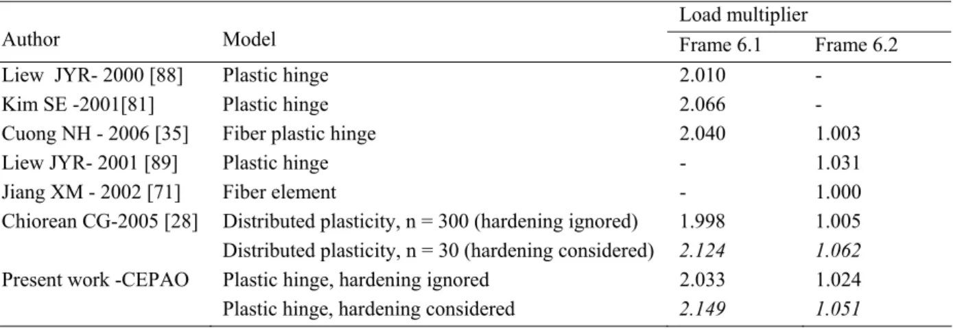
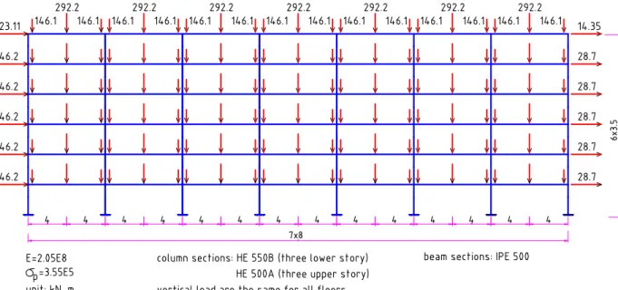
Figure
Documents relatifs
Within this study a discrete approach derived from the classical Discrete Element Method (DEM) was employed to describe the behaviour of snow in both the brittle and ductile
For instance, a peer that only expects to receive a message from channel a followed by a message from channel b cannot impose the reception order (the communication model will have
Empirical relationships have been determined for the latent and sensible heat fluxes as well as the total horizontal momentum flux and turbulent kinetic energy in a wind speed
Le Conseil supérieur de l'éducation Comité catholique Comité protestant Conseil supérieur de l'éducation Comité consultatif sur l'accessibilité financière aux études Commission
create biexcitons with energies up to six times that of the band gap by creating electron-hole pairs from the lowest valence and the highest conduction states taken within the
In pcn embryos arrested at globular stage, PIN1-GFP appeared in a broad central region of the embryo (Figure 9-1H and 1I), and the expression was seen in the vascular initials of
Using the commercial program Fluent, the predicted velocity magnitude contours, force coefficients and velocity fields are compared for the two cases (with and without free
Scaling laws based metamodels for the selection of the cooling strategy of electromechanical actuators in the early design stages.. Ion Hazyuk a,∗ , Marc Budinger a , Florian Sanchez
