Ecology and physiology of chaetognaths (semi-gelatinous zooplankton) in Arctic waters

Ecology of chaetognaths

(semi-gelatinous zooplankton) in Arctic waters

Thèse

Jordan Grigor

Doctorat interuniversitaire en océanographie

Philosophiæ doctor (Ph. D.)

Québec, Canada

Ecology of chaetognaths

(semi-gelatinous zooplankton) in Arctic waters

Thèse

Jordan Grigor

Sous la direction de :

iii

Résumé

Les chaetognathes sont d’importants membres des communautés mésozooplanctoniques de l’Arctique en ce qui a trait à l'abondance et à la biomasse. Les chaetognathes de l’Arctique se répartissent en trois espèces principales qui sont considérées comme étant strictement carnivores : Eukrohnia hamata, Parasagitta elegans et Pseudosagitta maxima. Cette étude utilise un ensemble de données de filet planctoniques recueillies sur une période de 5 ans dans les régions européennes, canadiennes et de l'Alaska de l’Arctique (2007, 2008, 2012, 2013, 2014) et comprend un cycle annuel complet dans l'Arctique canadien (2007-2008), le but étant d’améliorer notre compréhension sur les distributions, les cycles de vie et les stratégies d'alimentation du E. hamata et du P. elegans. Dans la présente thèse, les points suivants seront abordés : (1) la stratégie d'alimentation et la maturité du P. elegans dans l'Arctique européen durant la nuit polaire en 2012 et 2013, (2) les cycles de croissance et de reproduction, les stratégies d'alimentation et les distributions verticales du E. hamata et du

P. elegans dans l'Arctique canadien de 2007 à 2008, et (3) les différences spatiales dans les

stratégies d'alimentation du E. hamata et du P. elegans à l'automne 2014. Afin d’étudier leurs stratégies d'alimentation, des analyses de contenu du tube digestif ainsi que des techniques biochimiques ont été utilisées. Dans l'Arctique canadien, le E. hamata et le P. elegans vivent tous deux pendant environ 2 ans. Le P. elegans colonise principalement les eaux épipélagiques, tandis que le E. hamata colonise principalement les eaux mésopélagiques. Dans cette région, P. elegans se reproduit en continue de l'été au début de l'hiver, dans la période de forte biomasse de copépodes, qui constituent ses proies, dans les eaux proches de la surface, un mode de reproduction basé sur l’apport immédiat d’énergie. Cependant, les résultats ont révélé que E. hamata a engendré des couvées distinctes dont on peut voir l’évolution au cours de fenêtres de reproduction séparées, à la fois durant les périodes de printemps-été et d’automne-hiver, ce qui suggère une reproduction basée sur les réserves. Les taux de prédation quotidiens évalués à partir des analyses du contenu du tube digestif sont généralement restés faibles pour les deux espèces de chaetognathes. Toutefois, pour E.

hamata et P. elegans, les taux de prédation inférés en été-automne ont dépassé ceux de

l’hiver-printemps. Des études d’alimentation ont révélé que E. hamata consomme de la matière organique particulaire (éventuellement des chutes de neige marine) tout au long de l'année, mais surtout en été, alors que le P. elegans se nourrit différemment. Les deux espèces

iv

sont caractérisées par une forte croissance estivale. La croissance hivernale du P. elegans était grandement restreinte, tandis que celle du E hamata l’était moindrement. En somme, les différences dans la façon dont les lipides et la neige marine sont utilisés par les deux espèces pourraient expliquer les différences dans leurs cycles de reproduction et leurs patrons de croissance saisonnière.

v

Abstract

Chaetognaths are important members of Arctic mesozooplankton communities in terms of abundance and biomass. Despite this, the bulk of seasonal studies have focused on grazing copepods. Arctic chaetognaths comprise three major species which are thought to be strict carnivores: Eukrohnia hamata, Parasagitta elegans and Pseudosagitta maxima. This thesis uses datasets collected from plankton net sampling during five years in European, Canadian and Alaskan areas of the Arctic (2007, 2008, 2012, 2013, 2014) and includes a full annual cycle in the Canadian Arctic (2007-2008), the purpose being to improve our understanding of the distributions, life history and feeding strategies of E. hamata and P. elegans. The following topics are addressed: (1) the feeding strategy and maturity of P. elegans in the European Arctic during the polar night in 2012 and 2013; (2) the growth, breeding cycles, feeding strategies and vertical distributions of E. hamata and P. elegans, in the Canadian Arctic from 2007 to 2008; and (3) spatial differences in the feeding strategies of E. hamata and P. elegans in autumn 2014. To investigate feeding strategies, a combination of gut contents and biochemical techniques was used. In the Canadian Arctic, both E. hamata and

P. elegans live for around 2 years. P. elegans mainly colonized epi-pelagic waters, whereas E. hamata mainly colonized meso-pelagic waters. In this region, P. elegans reproduced

continuously from summer to early winter when copepod prey peak in near-surface waters. This is characteristic of income breeders. However, results for E. hamata revealed that this species spawned distinct and traceable broods during separate reproductive windows in both spring-summer and autumn-winter, suggesting capital breeding. Daily predation rates inferred from gut content analyses appeared to be generally low in the two chaetognath species, though inferred predation rates in summer-autumn exceeded those in winter-spring. Feeding studies revealed that E. hamata consumed particulate organic matter (possibly falling marine snow) throughout the year but especially in the summer, whereas P. elegans did not feed in this way. High summer growth seems to be a characteristic of both these species. Growth during winter was highly restricted in P. elegans, to a lesser extent in E.

hamata. In summary, differences in how lipids and marine snow are utilised by the two

vi

Table of contents

1. Chapter 1 – General Introduction 1

1.1 The Arctic Ocean 1 1.1.1 Physical environment 2 1.1.2 Arctic marine ecosystems 3 1.2 Zooplankton and their polar adaptations 5 1.3 Chaetognaths 8 1.3.1 Arctic species and distributions 9 1.3.2 Lifespans 10

1.3.3 Reproductive strategy 11

1.3.4 Oil vacuoles in Eukrohnia spp. 11

1.3.5 Feeding strategies and trophic importance 12

1.3.6 Fatty acids and stable isotopes 14

1.4 Climate change and other challenges for Arctic marine life 14

1.5 Study areas 17

1.6 Aims and objectives 18

2. Chapter 2 – Polar night ecology of a pelagic predator, the chaetognath Parasagitta elegans 20 2.1 Résumé 20 2.2 Abstract 21 2.3 Introduction 22 2.4 Method 23 2.4.1 Study area 23

2.4.2 Physical and biological environment 24

2.4.3 Zooplankton sampling 24

2.4.4 Sample processing 25

2.4.5 Gut content analyses 26

2.4.6 Food-containing ratio and feeding rate 26

2.4.7 Stable isotope analyses 27

2.4.8 Determination of trophic level 28

2.4.9 Fatty acid analyses 28

2.4.10 Mid-winter maturity status 29

2.5 Results 30

vii

2.5.2 Gut contents 32

2.5.3 Body composition 34

2.5.4 Mid-winter maturity status 36

2.6 Discussion 36

2.6.1 Studies during the polar night 36

2.6.2 Feeding activity and rates 36

2.6.3 Energetics 38

2.6.4 Lipid profile 38

2.6.5 Reproduction 40

2.7 Concluding remarks 41

3. Chapter 3 – Growth and reproduction of the chaetognaths Eukrohnia hamata and Parasagitta elegans in the Canadian Arctic Ocean: capital breeding versus income breeding 42 3.1 Résumé 42 3.2 Abstract 43 3.3 Introduction 44 3.4 Method 46 3.4.1 Study area 46 3.4.2 Sampling 47

3.4.3 Chaetognath body size and sampler efficiency 48

3.4.4 Hatching and cohort development 49

3.4.5 Estimation of maturity and oil vacuole area 50

3.4.6 Vertical distributions 50

3.5 Results 51

3.5.1 Physical environment and primary production in the Amundsen Gulf 51

3.5.2 Physical environment and primary production in autumn (other sampling locations) 51

3.5.3 Abundances and vertical distributions of chaetognath species 52

3.5.4 Length distributions and sampler efficiency 53

3.5.5 Timing of reproduction 54

3.5.6 Eukrohnia hamata length cohorts and life cycle 55

3.5.7 Parasagitta elegans length cohorts and life cycle 62

3.6 Discussion 67

3.6.1 Chaetognath cohort interpretation and lifespans 67

3.6.2 Resource partitioning in the sympatric Eukrohnia hamata and Parasagitta elegans 67

3.6.3 The potential role of lipid reserves: contrasting growth in the two species 69

3.6.4 Maturation 71

3.6.5 Capital versus income breeding in a warming Arctic 72

3.7 Conclusions 73

4. Chapter 4 – Feeding strategies of arctic chaetognaths: are they really “tigers of the plankton”? 74

viii 4.1 Résumé 74 4.2 Abstract 75 4.3 Introduction 76 4.4 Method 77 4.4.1 Study areas 77

4.4.2 Sampling in the Amundsen Gulf 79

4.4.3 Sampling in the Chukchi Sea and Baffin Bay 80

4.4.4 Abundance of zooplankton 80

4.4.5 Gut contents 81

4.4.6 Fatty acids 82

4.4.7 Carbon and nitrogen 82

4.5 Results 84

4.5.1 Amundsen Gulf 84

4.5.1.1 Phenology of algae blooms 84

4.5.1.2 Zooplankton community 84

4.5.1.3 Visible prey items and predation rates 86

4.5.1.4 Lipid droplets and detritus 87

4.5.1.5 Scanning Electron Microscope observations 89

4.5.2 Chukchi Sea and Baffin Bay 90

4.5.2.1 In-vitro feeding observations 90

4.5.2.2 Lipid amounts 90

4.5.2.3 Fatty acid profiles: species differences 91

4.5.2.4 Fatty acid profiles: station and regional differences in Eukrohnia hamata and Parasagitta elegans 91

4.5.2.5 Carbon and nitrogen isotopes 94

4.6 Discussion 96

4.6.1 Prey items 96

4.6.2 Predation rates 97

4.6.3 Omnivory in arctic chaetognaths 98

4.6.4 Fatty acids and stable isotopes confirm gut contents 99

4.6.4.1 18:1 (n-9)/(n-7) ratios and Calanus copepod FATMs 99

4.6.4.2 Algal FATMs 100

4.6.4.3 δ13_{C values 100}

4.6.4.4 δ15N values and inferred TLs 101

4.6.4.5 C/N ratios 101

4.6.5 Morphological explanations 102

4.7 Concluding remarks and future studies 102

5. Chapter 5 – General Conclusions 103

5.1 Resource use by arctic chaetognaths 103

5.2 Winter ecology in Svalbard 103

5.3 Life histories, habitats and spawning times 104

5.4 Food resources 105

5.5 Limitations of the study 107

ix

5.5.2 Stable isotopes and trophic levels 107

5.5.3 Length cohorts 108

5.6 Future research avenues 108

5.7 A note on climate change 109

Bibliography 110

Appendix A. Information on the zooplankton samples included in Chapter 2 126

Appendix B. Vertical profiles of temperature and salinity in Chapter 2 128

Appendix C. Stations sampled in Chapter 3 129

Appendix D. Vertical profiles of temperature, salinity and chlorophyll a in Chapter 3 131

Appendix E-1. Amundsen Gulf stations sampled in Chapter 4 132

x

List of tables

Table 2.1 Total water-column abundances (ind. m-3) of a polar night zooplankton community (Rijpfjorden 2012), ordered according to abundance per taxonomic group. Net sampling (Multi-Plankton Sampler; 0.25-m2 opening, 0.2-mm mesh) was used. As larger chaetognaths may have avoided the smaller MPS net (see Grigor et al. 2014), chaetognath abundances presented here are likely to be underestimates. Mean abundances for species and copepod stages were first calculated over two hauls (one at midday and the other at midnight at various depth intervals, see Appendix A), and data were summed across all sampling depths. Copepod stages are CI-CV, AM (adult male) and AF (adult female). Functional (feeding) groups were extracted from Søreide et al. (2003). “Small Calanoida” comprised the following taxa: Acartia longiremis, Aetideidae CI-CIII, Bradyidius similis, Microcalanus spp. and Pseudocalanus spp. Only taxa with abundances of ≥0.1 ind. m-3 _{are shown. 31} Table 2.2 Stable carbon and nitrogen isotope values for Parasagitta elegans sampled by the MIK (3.14-m2 opening, 1.5-mm mesh) at various trawl depths (20, 30, 35, 60, 75 and 225 m) in Isfjorden and Rijpfjorden (2012). The average δ13_{C and δ}15_{N composition (‰)} in replicate samples (usually three but six from 225 m in Rijpfjorden) containing 25 pooled individuals (10-50 mm), average proportions of animal dry weight (DW) comprising carbon and nitrogen (%), and C/N weight ratios. All values are accompanied by standard deviations. Trophic levels (TL) were calculated for P. elegans from each fjord from mean δ15_{N (‰) values (see ‘Method’). 34} Table 2.3 Average fatty acid profile for Parasagitta elegans in 2012. Results are given as average percentages of the various fatty acids identified across all samples from Isfjorden and Rijpfjorden (see ‘Method’), alongside the standard deviations. Only fatty acids with mean percentages of =>0.5 ± 0.1 across both fjords are shown. In Isfjorden, the mean percentages of 15:0 FA and 18.2(n-6) FA differed between sampling depths (indicated by a † symbol, one-way ANOVA, P ˂ 0.05). In Rijpfjorden, the proportion of every fatty acid was similar between sampling depths (one-way ANOVA, P ˃ 0.05). 35 Table 3.1 Timing of peak development of maturity features in autumn and spring broods of

Eukrohnia hamata and summer brood of Parasagitta elegans, and of the oil vacuole in E. hamata. Ages in months at peak development are given in parentheses. Monthly

collections consisted of up to 397 and 434 E. hamata individuals from its autumn and spring broods respectively, and 177 P. elegans. 59 Table 4.1 Composition of the mesozooplankton (30 most abundant taxa) sampled in the Amundsen Gulf from November 2007 to July 2008, based on data from 70 Multinet hauls. *Taxa could not be identified to species level. 85 Table 4.2 Frequency of first- and second-year Eukrohnia hamata individuals with green lipid droplets or macroaggregates in guts. Separate results are presented for the autumn (October) and spring (April) broods of E. hamata (see Chapter 3), from approximate month of hatching (no gut content data were available for October). 88

xi

Table 4.3 Mean sample lipid, fatty acid amounts and fatty acid proportions (± 1 SD) in (a)

Eukrohnia hamata and (b) Parasagitta elegans at different stations (stns) in autumn

2014. Sampling locations are abbreviated: CS, Chukchi Sea; SIF, Scott Inlet Fjord; GF, Gibbs Fjord; SBB, southern Baffin Bay. Also: number (n) of samples analysed and chaetognaths per sample, and chaetognath body lengths in mm. † Significant species

differences (P ≤ 0.05). 92

Table 4.4 Mean sample carbon (C) and nitrogen (N) masses, C/N ratios, δ13C and δ15N values and derived trophic levels (TLs) (± 1 SD) in Eukrohnia hamata and Parasagitta elegans at different stations in autumn 2014. Sampling locations are abbreviated: CS, Chukchi Sea; SIF, Scott Inlet Fjord; GF, Gibbs Fjord; SBB, southern Baffin Bay. Also: number (n) of samples analysed and chaetognaths per sample, as well as body lengths of

xii

List of figures

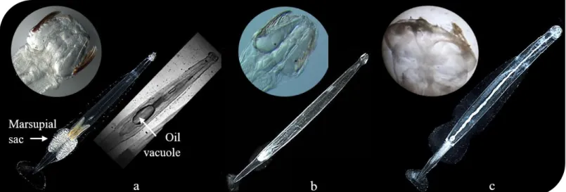
Figure 1.1 Bathymetric map of the central Arctic Ocean and several marginal seas (http://recherchespolaires.inist.fr/?L-ocean-Arctique-physiographie). 1 Figure 1.2 Water masses in the Arctic Ocean. Reproduced from Stein & Macdonald (2004).2 Figure 1.3 The planktonic food web showing protozoan and metazoan consumers at arrow caps. Adapted from Hopcroft et al. (2008). 4 Figure 1.4 Photographs of living holo-zooplankton captured in-situ by a zooplankton imager (Lightframe On-sight Key Species Investigation System; Schmid et al. 2016), during deployments in the Canadian Arctic (summer 2014). 6 Figure 1.5 Typical physiology of a chaetognath belonging to the family Sagittidae. Reproduced from Margulis & Chapman (2010). 8 Figure 1.6 Photographs of the heads and the bodies of the major arctic chaetognaths. (a)

Eukrohnia hamata with characteristic marsupial sac and oil vacuole, (b) and (c)

Parasagitta elegans and Pseudosagitta maxima without marsupial sacs and oil vacuoles.

All images except P. maxima head from:

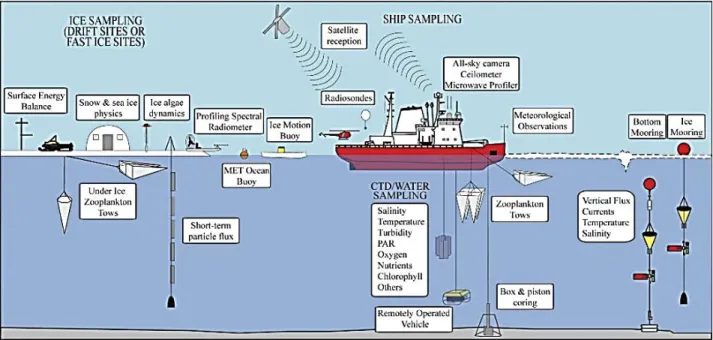
http://www.arcodiv.org/watercolumn/Chaetognaths.html (courtesy of Russ Hopcroft). 9 Figure 1.7 Photograph of a chaetognath’s head taken by Scanning Electron Microscopy (left) with parts labelled (right). Reproduced from Bieri & Thuesen (1990). 12 Figure 1.8 Diagram illustrating the wide variety of sampling activities conducted during the Circumpolar Flaw Lead System Study (2007-2008) from the icebreaker CCGS

Amundsen and at an ice camp, in order to study Arctic systems. Reproduced from Barber

et al. (2010). 18

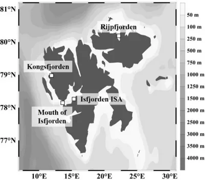
Figure 2.1 Map showing the locations of the stations sampled for chaetognaths in January

2012 and 2013. 24

Figure 2.2 Proportions (%) of Parasagitta elegans individuals per haul with gut contents (FCRmax), identifiable prey (FCRmin), and empty guts in each fjord. The horizontal line inside each boxplot shows the median of the proportions over multiple haul samples in a fjord. The lower and upper boxes show the lower and upper quartiles, respectively, and the vertical lines outside the boxes the differences between these quartiles and the lowest and highest proportions observed. Each dot represents an outlying data point. nhauls = numbers of hauls for each fjord. Hauls with ˂3 individuals analysed were not included. As only one haul was analysed for Rijpfjorden in 2013, full boxplots could not be shown. See Appendix A for numbers of individuals analysed per haul. 32

xiii

Figure 2.3 Proportions (%) of feeding Parasagitta elegans individuals per haul in each fjord with different types of gut content. For details on the features of the boxplots and the

data, see Figure 2.2. 33

Figure 2.4 Gut contents in ascending head width size classes: proportions of Parasagitta

elegans (%) per haul with gut contents and of feeders with each gut content type.

Includes all dissected specimens from Isfjorden (50 individuals, 4 hauls) and Rijpfjorden (152 individuals, 13 hauls) in 2012. For details on the features of the boxplots and the data, see Figure 2.2. ninds. = total numbers of individuals for each size class. 33 Figure 3.1 Bathymetric maps of the Canadian Arctic Ocean indicating the regions, and positions of stations (black circles) where chaetognaths were sampled from August 2007 to September 2008. Station IDs provided. 47 Figure 3.2 Illustrations and photographs of Eukrohnia hamata and Parasagitta elegans. (a) Diagrams of the two species indicating maturity features and the centrally-positioned oil vacuole in E. hamata. (b) Photographs of live E. hamata (top) and P. elegans (bottom) taken in-situ by a zooplankton imager (Schmid et al. 2016) in the Canadian Arctic. Specimens ~20 mm. (c) Photograph of oocytes in a stained P. elegans individual. (d) Photograph of ovaries in an E. hamata individual (imaged in-situ). (e) Photograph of tail sperm, seminal vesicles and seminal receptacles in a stained P. elegans individual. 49 Figure 3.3 Relative frequency of Eukrohnia hamata, Parasagitta elegans and Pseudosagitta

maxima in relation to bottom depth at Amundsen Gulf stations. Multinet and

square-conical net collections included. b) Weighted mean depths of E. hamata and P. elegans normalized relative to the bottom depth at Amundsen Gulf stations (see ‘Method’). Multinet collections. Standard deviation bars also given. The blue area indicates the Pacific Halocline (60-200 m) and the red area indicates the Atlantic Layer ˃ 200 m

(Geoffroy et al. 2011). 53

Figure 3.4 Length frequency (mean % ± 1 SD) distributions of Eukrohnia hamata and

Parasagitta elegans in the square-conical (S-C) net (1 m2 aperture, 200 µm mesh) and Multinet (0.5 m2 aperture, 200 µm mesh) in the Amundsen Gulf. Note the different scales for the two species. k is the number of collections. 54 Figure 3.5 Abundance (mean numbers m-2 + 1 SD) of newborn Eukrohnia hamata and

Parasagitta elegans (body lengths of 2-4 mm) in monthly Multinet deployments from

October to September. August 2007 was inserted between July and September 2008 to provide a complete composite of the annual cycle. Number of collections shown above bars. The solid horizontal bar above month labels indicates sampling in the Amundsen

Gulf. 55

Figure 3.6 Monthly length frequency distributions of Eukrohnia hamata. Frequencies of newborns highlighted in orange. Visually identified length cohorts shown as normal distributions (in red) with red dots indicating the mean length. Each of the five cohorts is labelled with a capital E and a number from oldest (1) to youngest (5). Blue line is the

xiv

total distribution obtained by summing the modelled distributions. Chi-square values for the goodness-of-fit of the total distribution to the data are given. Sampling regions are abbreviated in each panel: PC, Parry Channel; AG, Amundsen Gulf; BB, Baffin Bay. k is the number of collections and n the number of length measurements included (see

‘Method’). 56

Figure 3.7 a) Monthly mean length (± 1 SD) of the five cohorts of Eukrohnia hamata starting from a major birth month; b) Composite growth trajectories of the autumn brood (born in October) and spring brood (born in April) assuming a 2-y lifespan; c) Growth-age curves of the autumn and spring broods. Circles show mean values of each characteristic

(± 1 SD shown as ribbons). 58

Figure 3.8 Development of sexual features (a, oocyte number; b, ovary length; d, sperm load; e, seminal vesicle width; f, seminal receptacle diameter) and oil vacuole area (c) with length for the autumn and spring broods of Eukrohnia hamata. Circles show mean values of each characteristic (± 1 SD shown as ribbons). Vertical line indicates average length (15.4 mm) at one year of age. Maturity results for each brood were obtained from the analyses of up to 283 individuals from each 1 mm length class. 60 Figure 3.9 Mean frequency (± 1 SD) of Eukrohnia hamata with oil in vacuole and/or digestive tract by months. Number of water column collections shown inside bar (33 –

446 individuals per haul). 61

Figure 3.10 Abundances (ind. m-3) of Eukrohnia hamata age classes in discrete depth layers of the Amundsen Gulf, characterized by their mid-points (black squares). Top panels: autumn brood individuals. Bottom panels: spring brood individuals. Seabed shown in brown, unsampled sections of the water column in gray. See ‘Method’ for further details.

62 Figure 3.11 Monthly length frequency distributions of Parasagitta elegans. Frequencies of newborns highlighted in orange. Visually identified length cohorts shown as normal distributions (in red) with red dots indicating the mean length. Each of the three cohorts is labelled with a capital P and a number from oldest (1) to youngest (3). Blue line is the total distribution obtained by summing the modelled distributions. Chi-square values for the goodness-of-fit of the total distribution to the data are given. Sampling regions are abbreviated in each panel: NF, Nachvak Fjord; PC, Parry Channel; AG, Amundsen Gulf; BB, Baffin Bay. k is the number of collections and n the number of length measurements

included (see ‘Method’). 63

Figure 3.12 a) Monthly mean length (± 1 SD) of the three cohorts of Parasagitta elegans starting from a major birth month; b) Composite growth trajectory of the single brood.64 Figure 3.13 Development of sexual features (a, oocyte number; b, ovary length; c, sperm load; d, seminal vesicle width; e, seminal receptacle diameter) with length in Parasagitta

xv

Vertical line indicates average length (20.7 mm) at one year of age. Maturity results were obtained from the analyses of up to 63 individuals from each 1 mm length class. 65 Figure 3.14 Abundances (ind. m-3) of Parasagitta elegans age classes in discrete depth layers of the Amundsen Gulf, characterized by their mid-points (black squares). Seabed shown in brown, unsampled sections of the water column in gray. See ‘Method’ for further

details. 66

Figure 4.1 Bathymetric maps of the Arctic Ocean, showing the positions and IDs of sampling stations (black circles) in (a) Amundsen Gulf, (b) north-eastern Chukchi Sea and (c) Baffin Bay (SIF = Scott Inlet Fjord; GF = Gibbs Fjord; SBB = southern Baffin Bay). Details of sampling stations are shown in Appendices E-1 and E-2. 79 Figure 4.2 Vertical distributions of chlorophyll a biomass (mg m-3) in the upper 200 m of the water column along the ship track from November 2007 to July 2008 in the Amundsen Gulf. Black dots indicate sampling depths. Details of sampling stations are shown in Appendix E-1. Chl a data were provided by Michel Gosselin (Université du Québec à

Rimouski). 84

Figure 4.3 Average number of prey per chaetognath gut (npc) in square-conical (S-C) net and Multinet collections from November 2007 to August 2008 in the Amundsen Gulf. Numbers of individuals shown above data points. k is the number of collections. Inset bottom: photograph of a Parasagitta elegans specimen (12 mm) with a relatively large

Pseudocalanus spp. copepod in the gut (from November 2 2007). 86 Figure 4.4 Photographs of substantial amounts of green macroaggregates (˃ 500 µm) in the guts of Eukrohnia hamata, but not in the guts of Parasagitta elegans. Specimens from the Amundsen Gulf on May 31 2008 (20-40 m depth), 20-30 mm. 87 Figure 4.5 Scanning Electron Microscope photographs of some items in Eukrohnia hamata guts (left box) and Parasagitta elegans guts (right box), in different months. Examples: hooks of a chaetognath, and mandibles of copepods (arrow caps). Specimens 20-30 mm.

89 Figure 4.6 Photographs of live Eukrohnia hamata individuals consuming green macroaggregates in-vitro in the Chukchi Sea. Specimens 20-30 mm. Bottom right: An inverted microscope photograph of phytoplankton such as Ceratium spp. in one gut. 90 Figure 4.7 Fatty acid biomarkers in Eukrohnia hamata and Parasagitta elegans at different stations in autumn 2014. Sampling locations are abbreviated: CS, Chukchi Sea; SIF, Scott Inlet Fjord; GF, Gibbs Fjord; SBB, southern Baffin Bay. From top panel to bottom panel: mean ratios of the carnivory biomarker 18:1 (n-9)/(n-7), mean proportions of the

Calanus biomarkers ΣC20:1+C22:1 MUFA, and mean ratios of the algal biomarker

xvi

Figure 4.8 Mean sample δ13C and δ15N values and corresponding trophic levels (± 1 SD) of

Eukrohnia hamata and Parasagitta elegans. Station IDs shown next to data points.

Results from Chukchi Sea stations inside red oval. Results from Baffin Bay region stations inside blue oval (locations are abbreviated: SIF, Scott Inlet Fjord; GF, Gibbs

xvii

Dedicated to the memory of Helen McMahon, my granny, who made it possible for me to first pursue my interest in the Arctic regions.

23 August 1929 – 25 March 2015

Angelina Kraft

xviii

Acknowledgements

I am now nearing the end of my journey to gain a Ph. D. in Oceanography, and there are several people who have supported me whom I would like to acknowledge in this thesis. Firstly, I would like to thank my director of research, Dr. Louis Fortier for allowing me to realize this project on the enigmatic chaetognaths. I would also like to thank Louis for giving me opportunities to attend and present my research at several national and international conferences, to voyage to the Arctic/sub-Arctic on three separate research cruises, and for the many ways in which he helped me improve my experience in scientific writing. Thanks to Drs. Jean-Éric Tremblay, Guillaume Massé and Stéphane Plourde for evaluating the ‘dépôt initial’ of my thesis and thesis defense presentation, and providing useful suggestions for improvements. Thanks also to Dr. Maurice Levasseur for participating in my Ph. D. committee, and to Dr. Ladd Johnson for presiding over my defense presentation.

I express my gratitude to my colleagues Drs. Øystein Varpe (UNIS), Stig-Falk Petersen (Akvaplan-niva), Dominique Robert, Eric Rehm, Guillaume Massé and Marcel Babin (Université Laval), Roxane Barthélémy and Jean-Paul Casanova (Aix-Marseille Université), and Mrs. Ariane Beauféray (Université Laval), all of whom helped to shape the direction of this thesis. I would like to specifically acknowledge Dr. Øystein Varpe who has consistently shown a keen interest in my research, and been happy to offer constructive ideas and suggestions. Thanks to Drs. Catherine Lalande (Université Laval), and Tara Connelly (Memorial University of Newfoundland), as well as anonymous journal referees for Polar Biology and Journal of Plankton Research, for offering valuable comments on chapters.

I am grateful to the crew and scientific staff on expeditions with R/V Helmer Hanssen and CCGS Amundsen for research support. Dr. Gérald Darnis’ assiduity onboard CCGS

Amundsen, and in the laboratory, was fundamental to the success of zooplankton sections of

the CFL project. Mr. Carl Ballantine collected samples from Svalbard in 2013. I greatly appreciate the hard work of my student assistants; Mrs. Ariane Beauféray, Miss. Marianne Caouette, Miss. Vicky St-Onge, Mr. Joël-Fortin Mongeau and Mr. Pierre-Olivier Sauvageau, for helping me to analyse the vast number of chaetognaths included in this thesis. Sincere thanks also to the following individuals and lab groups for analysing fatty acids and stable

xix

isotopes: Dr. Guillaume Massé, Miss Caroline Guilmette, Mr. Jonathan Gagnon, the Institute for Energy Technology and UNILAB in Norway. Thanks to Drs. Jean-Éric Tremblay and Michel Gosselin, and Miss Marjolaine Blais for contributing environmental datasets.

I would like to thank my close friends Moritz Schmid, Kai Shapiro and Sophie Regueiro for their moral support during the most challenging stages of my Ph. D. Many others, including Cyril Aubry, Kevin Gonthier, Arnaud Pourchez, Noémie Friscourt, Max Geoffroy and other members of the Fortier lab, have given me great memories from my time in Québec and Canada. I am grateful to my parents (Ali and Dave), sister Ara, as well as the rest of my family, who were ready to Skype at a moment’s notice and were always ready to offer support, advice and encouragement. Thanks to the School for Science and Math at Vanderbilt (Nashville, USA) for more recently giving me the opportunity to share my passion for the polar regions with the next generation of scientists.

Bursaries from Takuvik and Québec-Océan allowed me to keep the focus on all my doctoral activities and reach these final stages of my Ph. D. course.

xx

Foreword

This doctoral thesis comprises a General Introduction (Chapter 1), three scientific articles (Chapters 2, 3 and 4), and a number of General Conclusions relating to the objectives of the thesis (Chapter 5). Chapter 2 is published in Polar Biology as part of a Special Issue on Polar Night ecology. Chapters 3 and 4 are currently in preparation for publication:

Chapter 2

Grigor J.J., Marais A., Falk-Petersen S., Varpe Ø. (2015) Polar night ecology of a pelagic

predator, the chaetognath Parasagitta elegans. Polar Biology 38:87-98 (reproduced with permission of the publisher). Minor formatting changes have been made to the material published in Polar Biology, to ensure compatibility with the other chapters in this thesis (e.g. species names are written out in full the first time they are used in every new paragraph, and thereafter abbreviated to their shorter form. Citations follow the same format as in the other chapters).

Chapter 3

Grigor J.J., Schmid M.S., Fortier L. Growth and reproduction of the chaetognaths

Eukrohnia hamata and Parasagitta elegans in the Canadian Arctic Ocean: capital breeding

versus income breeding. This has been revised and recently re-submitted to Journal of

Plankton Research.

Chapter 4

Grigor J.J., Barthélémy R.-M., Massé G., Casanova J.-P., Fortier L. Feeding strategies of

arctic chaetognaths: are they really “tigers of the plankton”? This will be submitted to Journal

of Plankton Research.

The aims and objectives of this thesis were designed by myself. All the analyses were performed by myself (or by students under my supervision). To collect material for the thesis, I participated in research cruises in winter 2012, autumn 2013 and autumn 2014. Chapters 2-4 have benefited from the corrections and comments of my co-authors. Results of these three

xxi

chapters have been presented at the following national and international scientific conferences:

[9] Grigor J.J., Marais A.E., Schmid M.S., Varpe Ø., Fortier L. (2015) Ecology of arrow worms in the Arctic: are they really “tigers of the zooplankton”?? APECS Online

Conference – New Perspectives in the Polar Sciences

[8] Grigor J.J., Varpe Ø., Marais A.E., Schmid M.S., Rehm E., Fortier L. (2014) Ecology of arrow worms in the Arctic: are they really “tigers of the zooplankton”?? Arctic Change

Conference (Ottawa, Canada)

[7] Grigor J.J., Marais A.E., Schmid M.S., Rehm E., Fortier L. (2014) Arrow worm ecology in the Canadian Arctic. Arctic Change Conference (Ottawa, Canada)

[6] Grigor J.J., Marais A.E., Schmid M.S., Rehm E., Fortier L. (2014) Arrow worm ecology in the Canadian Arctic. Assemblée générale annuelle de Québec-Océan (Rivière-du-Loup, Canada)

[5] Grigor J.J., Marais A.E., Schmid M.S., Fortier L. (2013) Seasonal ecologies of chaetognaths (gelatinous zooplankton) in the Canadian Arctic. ArcticNet Annual Science

Meeting (Halifax, Canada) *Awarded best poster in its category: Marine Natural Science

[4] Grigor J.J., Søreide J.E., Varpe Ø., Fortier L. (2013) Seasonal ecology and life history strategies of the chaetognath Parasagitta elegans in the Canadian and European Arctic: The story so far. Assemblée générale annuelle de Québec-Océan (Rivière-du-Loup, Canada)

[3] Grigor J.J., Søreide J.E., Varpe Ø. (2013) The annual routine of a predatory arctic chaetognath in a highly seasonal environment. Arctic Frontiers: Geopolitics and marine

xxii

[2] Grigor J.J., Søreide J.E., Varpe Ø. (2012) The annual routine of a predatory zooplankter in a highly-seasonal Arctic environment. Annual ArcticNet Science Meeting (Vancouver, Canada)

[1] Grigor J.J., Søreide J.E., Varpe Ø. (2012) The annual routine of a predatory zooplankter in a highly-seasonal Arctic environment. Québec Océan 10-yr conference: A

reality check on oceans’ health (Montreal, Canada)

During my Ph. D., I participated as a co-author in the writing of one scientific article that used an underwater camera system, the Lightframe On-sight Keyspecies Investigation system (LOKI), to capture excellent images of zooplankton and document their fine-scale vertical distributions. The study also developed a model to automatically identify the species and stages of imaged animals:

[1] Schmid M.S., Aubry C., Grigor J.J., Fortier L. (2016) The LOKI underwater imaging system and an automatic identification model for the detection of zooplankton taxa in the Arctic Ocean. Methods in Oceanography 15:129-160

1

1. Chapter 1 – General introduction

1.1 The Arctic Ocean

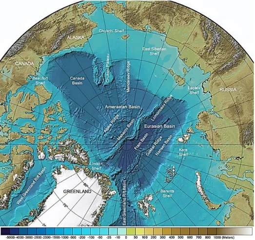
The Arctic area is characterized by strong seasonal cycles in solar radiation and surface sea-ice cover. The sun remains more than 12° below the horizon at the height of winter (the ‘polar night’) and does not set at the height of summer (the ‘midnight sun’). The Arctic Ocean covers an area of 14 million km2 (Huntington & Weller 2005) and is divided by a submarine ridge of continental crust (the Lomonosov Ridge) into two major basins, the Eurasian and Amerasian Basins (Figure 1.1). Vast continental shelves comprise 50 % of the Arctic Ocean area (Figure 1.1), and these are amongst its most biologically productive areas (Sakshaug 2003, see ‘Marine ecosystems’ section).

Figure 1.1 Bathymetric map of the central Arctic Ocean and several marginal seas

2

1.1.1 Physical environment

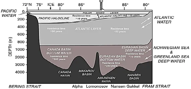
Through dynamic and thermodynamic processes (movement, growth and melt), the extent of surface sea-ice increases to its maximum in March and declines thereafter towards its minimum in September (Stroeve et al. 2008). Sea-ice acts as a barrier between the underlying ocean and the atmosphere affecting heat exchange and the transmission of light that algae in the water require for primary production. Sea-ice is also a habitat for several specialized fish, seabird and mammal species, and influences global climate. Ice formation in key locations is important for the formation of cold and highly saline water. This briny water sinks, initiating deep-water currents that move into other oceans as an integral part of the ‘thermohaline circulation’ (Loeng et al. 2005). Surface water/ice follows two important surface currents: in the western Arctic the clockwise-turning Beaufort Gyre; and in the eastern Arctic the Transpolar Drift, which exports ice into the Atlantic (Stein & Macdonald 2004). Freshwater contributions from ice melt, precipitation and large non-freezing rivers (e.g. Ob and Yenisei in Eurasia, the McKenzie and Yukon in N. America), increase the buoyancy of surface waters (i.e. the Polar Mixed Layer). Great volumes of warm, relatively saline Atlantic water, also enter the Eurasian Basin through the deep (2600 m) Fram Strait (Figure 1.2) and the Barents Sea. Lower volumes of cold, relatively fresh Pacific water, are supplied to the Amerasian Basin through the 45 m-deep Bering Strait (Stein & Macdonald 2004, Figure 1.2).

3

In the Amerasian Basin, the Atlantic Water cools and becomes denser, plunging below the Pacific water to depths ˃200 m, where it resides for ~30 years (Stein & Macdonald 2004, Figure 1.2). The inflows of Pacific water in the Amerasian Basin and of Atlantic water in the Eurasian basin create salinity gradients (haloclines) that protect sea-ice from warm waters below (Winsor & Bjork 2000). Arctic deep water (cold and relatively saline), can occur below 900 m in the deep areas of the basins, where it has a residence time of 75-300 years (Stein & Macdonald 2004, Figure 1.2).

1.1.2 Arctic marine ecosystems

Arctic marine ecosystems are considered less complex than most temperate and tropical systems, with lower productivity and biodiversity in general (Loeng et al. 2005). In Arctic marine ecosystems, extreme cycles in solar illumination and sea-ice cover lead to strong seasonal cycles in primary production by autotrophic algae, with a considerable reduction in winter (Ji et al. 2013). However, biological hotspots occur where a good nutrient supply to surface waters supports high primary productivity. For instance, large blooms of phytoplankton in some parts of the Chukchi Sea near Alaska support sizable communities of invertebrates, both in the water column and on the seabed (Hopcroft et al. 2004, Grebmeier et al. 2006, Nishino et al. 2016). Furthermore, polynyas (permanently open water areas otherwise surrounded by sea-ice) are viewed as biological ‘oases’, with phytoplankton blooms occurring in polynyas earlier in the season than in any surrounding areas (Ingram et al. 2002, Hannah et al. 2009). This provides less-seasonally restricted access to food for grazers and in turn their predators. Polynyas can be formed by the upwelling of warm seawater which prevents ice from forming (i.e. sensible heat polynya), and/or by the influence of wind in driving ice away (i.e. latent heat polynya; Hannah et al. 2009). The large North Water Polynya in northern Baffin Bay (Canadian Arctic) is mainly a latent heat polynya in winter and spring, however, sensible heat is also important for its growth in late spring (Ingram et al. 2002).

In ice-covered seas, a bloom of under-ice algae is initiated during spring which is then succeeded by a bloom of pelagic phytoplankton when the ice retreats in the spring/summer.

4

Some locations can have another distinct phytoplankton bloom in autumn (Ardyna et al. 2014). Increases in the occurrence of autumn blooms across the Arctic may be a symptom of global warming (see ‘Climate change and other challenges for Arctic marine life’ section). On average, phytoplankton production is higher (12 to 50 g C m-2 yr-1) than ice algae production (5 to 10 g C m-2 _yr-1_{). However, ice algae production exceeds that of} phytoplankton in locations with thick multi-year ice cover (Legendre et al. 1992, Leu et al. 2011). Bloom phenology varies with latitude and timing of open water (Zenkevich 1963, Falk-Petersen et al. 2009, Tremblay et al. 2012), and the magnitude of a phytoplankton bloom during the ice-free period is determined by nitrogen availability (Tremblay & Gagnon 2009), and also influenced by zooplankton grazing (e.g. Banse 2013).

Arctic marine ecosystems contain at least 5000 species of invertebrate animal taxa from 24 phyla (Hoberg et al. 2013 and references therein), 91 % of which are associated with the seabed (i.e. ‘benthic’), 8 % with the water column (i.e. ‘pelagic’) and 1 % with the sea-ice (i.e. ‘sympagic’). Copepods belonging to the genus Calanus (Figure 1.3) are known as ‘key species’ in the Arctic seas. They convert carbohydrates and proteins taken up from the algae into high-energy lipids (wax esters) that comprise the main energy source within the food web (e.g. Falk-Petersen et al. 2009).

Figure 1.3 The planktonic food web showing

protozoan and metazoan consumers at arrow caps. Adapted from Hopcroft et al. (2008).

5

Amongst the vertebrates, up to 250 fish species reside in the Arctic area defined by the Conservation of Arctic Flora and Fauna (an Arctic Council Working Group), for part or all of the year (Hoberg et al. 2013). The polar cod Boreogadus saida is an endemic species which can channel up to ~75 % of energy flow from zooplankton to vertebrate predators (Welch et al. 1992). In addition, 35 species of mammals and 60 species of seabirds are observed in Arctic waters, with the Baffin Bay little auk population considered to be the largest seabird population in the world (Hoberg et al. 2013). Heterotrophic microbes and protists (Figure 1.3) remineralize dissolved organic carbon (˂0.45 µm) excreted from these consumers into inorganic forms of carbon which can then be taken up again by protozoans (Hopcroft et al. 2008).

1.2 Zooplankton and their polar adaptations

Zooplankton are aquatic animals with body sizes ˂0.002 mm to ˃200 mm which have limited ability to control their horizontal positions against water currents. As zooplankton have little capacity to evade warming waters and are typically not harvested by humans, variations in their distribution or phenology may strongly herald climate change effects (Richardson 2008). Zooplankters include herbivores, omnivores and carnivores, and are food for a wide diversity of invertebrate and vertebrate predators. Zooplankton fecal pellets can be an important source of carbon sequestration (e.g. Wassmann et al. 1999). However, fecal pellets excreted in epi-pelagic waters are typically removed rapidly in surface waters. This is due to degradation by bacteria, protozooplankton and copepods (Morata & Seuthe 2004, Turner 2015). Copepods, chaetognaths and other zooplankters are classified as ‘holoplankton’ taxa (that drift in the sea throughout their entire life cycle). In contrast, a variety of fish, decapods and other species are plankton only when they are larvae (‘meroplankton’), before then continuing life as nekton or benthos (Stübner et al. 2016). Some zooplankton species are capable of migrating considerable distances through the water column over day-night, seasonal or ontogenetic cycles. These behaviors may be associated with finding food, avoiding predation, or gaining an energy bonus from resting in colder waters, and they alter the spatial distributions of food, materials and energy (Longhurst et al. 1984, Haney 1988).

6

Arctic zooplankton biomass is typically dominated by Calanus copepods, followed by non-copepod taxa such as amphipods and chaetognaths (Figure 1.4). Zooplankton abundance is dominated by small cyclopoid and calanoid copepods including Oithona similis and

Pseudocalanus spp., amongst others (e.g. Søreide et al. 2003, Hopcroft et al. 2004, Darnis &

Fortier 2014). For stable co-existence, similar species must occupy slightly different ecological niches, efficiently partition available food and share habitat resources (Gause 1934, Ross 1986).

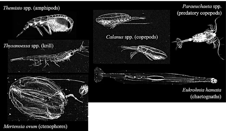
Figure 1.4 Photographs of living holo-zooplankton captured in-situ by a zooplankton imager

(Lightframe On-sight Key Species Investigation System; Schmid et al. 2016), during deployments in the Canadian Arctic (summer 2014).

Due to reduced growth rates in colder temperatures, zooplankton and other polar invertebrates often have longer lives and they reach maturity at older ages than those at lower latitudes (Hoberg et al. 2013). High-latitude zooplankton display a range of adaptations to a seasonal food source associated with, for instance, the timing and extent of growth and

7

reproduction, diapause, lipid content and feeding strategy (e.g. Conover 1988, Falk-Petersen et al. 2009, Varpe 2012, Grigor et al. 2014).

For grazers, such as Calanus glacialis, timing their growth and reproduction to coincide with the ice algae bloom can be of the utmost importance, as it would enable offspring to hatch ~3 weeks later during the phytoplankton bloom (Søreide et al. 2010, Leu et al. 2011, Daase et al. 2013). The high-quality food provided during this latter bloom allows for critical early growth of copepod offspring, without risk of starvation. Such a ‘match’ between the development of primary production and copepod offspring benefits copepod populations and the food web in general. However, in cases where offspring hatch before or after the peak of the phytoplankton bloom, they miss the phytoplankton food needed for healthy growth (Søreide et al. 2010, Leu et al. 2011). Such a ‘mismatch’ scenario has been shown to drastically reduce Calanus biomass (Leu et al. 2011).

Storage lipids are important for Arctic organisms, in which they may be used to fuel one or more of the following processes; basal metabolism, growth, maturation and reproduction (Kattner et al. 2007). Wax esters (comprising one fatty acid and one fatty alcohol) are the main long-term energy deposit in zooplankton, whereas triacylglycerols (comprising three hydrocarbon chains on a glycerol backbone) provide energy for activities in the short term (Lee et al. 2006). In winter, Calanus copepods and other grazers survive by entering diapause in relatively deep waters during which time accumulated wax ester stores are metabolized for energy. Capital breeders (e.g. C. hyperboreus) use their wax esters to fuel reproduction, and can produce offspring earlier in the season giving them a longer time to develop their energy reserves, required for surviving the next winter. Reproductive fitness is also improved (Varpe et al. 2007). Income breeders need recent food to reproduce, and mixed capital-income breeders use a combination of the two strategies (e.g. Sainmont et al. 2014a). Carnivores are assumed to have a low capacity for long-term energy storage (Hagen 1999), however, this may not be true for some species. Carnivorous and omnivorous zooplankters, like amphipods (Figure 1.4) are also assumed to feed opportunistically year-round (Hagen 1999).

8

1.3 Chaetognaths

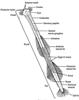
Chaetognaths (Figure 1.5) are a phylum of semi-gelatinous (dry weight ˃5 % wet weight; Larson 1986) marine mesozooplankton. They are represented worldwide by at least 127 pelagic and benthic species from 23 genera with body lengths 2-120 mm (e.g. Bone et al. 1991, Foster 2011). The name ‘chaetognath’ (Chaeto = bristle, gnath = jaw) relates to the presence of hooks on the head (Figure 1.5). Chaetognaths are also known as ‘arrow worms’ due to their lean appearance and rapid motion. These coelomates have existed from the Middle Cambrian and possibly before then (Walcott 1911). The global biomass of chaetognaths has been estimated at 10-30 % of that of copepods (Bone et al. 1991). The majority of species are residents of the upper 200 m of the water column (i.e. epi-pelagic; Pierrot-Bults & Nair 1991).

Figure 1.5 Typical physiology of a chaetognath belonging to the family Sagittidae.

Reproduced from Margulis & Chapman (2010).

Chaetognaths occur in the diets of zooplankton such as amphipods (Gibbons et al. 1992), jellyfish (e.g. Zavolokin et al. 2008) and other chaetognaths (e.g. Pearre 1982), and recently have received attention as the preferred prey for the larvae of tropical fish and commercially

9

important decapods (e.g. Sampey et al. 2007, Saunders et al. 2012). In the Arctic, fish such as the polar cod (Rand et al. 2013), seabirds such as the little auk (Mehlum & Gabrielsen 1993) and baleen whales (Pomerleau et al. 2012), feed on chaetognaths. Suthers et al. (2009) described chaetognaths as “the tigers of the plankton”. Animals in the phylum are generally thought to be opportunistic, but strict carnivores (Marazzo et al. 1997). For further details, see ‘Feeding strategies and trophic importance’ section.

1.3.1 Arctic species and distributions

In contrast to the high chaetognath diversity observed in other seas (e.g. De Souza et al. 2014), only three major species (Eukrohnia hamata, Parasagitta elegans and Pseudosagitta

maxima) are frequently reported in Arctic plankton surveys (e.g. Kramp 1939, Buchanan &

Sekerak 1982, Sameoto 1987, Figure 1.6). Another two species have been detected in Arctic bathy-pelagic surveys; Heterokrohnia involucrum (Dawson 1968) and H. mirabilis (Kapp 1991). Kosobokova & Hopcroft (2009) reported that chaetognaths represented, on average, about 13 % of the zooplankton biomass in the Canadian Arctic in summer 2005.

Figure 1.6 Photographs of the heads and the bodies of the major arctic chaetognaths. (a)

Eukrohnia hamata with characteristic marsupial sac and oil vacuole, (b) and (c) Parasagitta

elegans and Pseudosagitta maxima without marsupial sacs and oil vacuoles.

All images except P. maxima head from:

10

Parasagitta elegans (previously Sagitta) is restricted to the North Atlantic, North Pacific and

Arctic Oceans, with its lower distribution limit at 41°N and a northern limit short of the central Arctic basin (e.g. Bogorov 1946, Bieri 1959, Grainger 1959). It is generally an epi-pelagic, neritic species throughout most of its range (e.g. Terazaki 2004). Terazaki (2004) described P. elegans as the best-studied chaetognath species. In contrast to P. elegans,

Eukrohnia hamata and Pseudosagitta maxima are cosmopolitan species occurring in all

oceans, with predominantly meso- or bathy-pelagic affinities (e.g. Bigelow 1926, Bieri 1959, Cheney 1976, Thuesen et al. 1993). All three species occasionally co-occur at epi-pelagic depths in the Arctic (e.g. Alvarino 1964, Hopcroft et al. 2005, Bieri 1959). The life cycle and feeding strategy of E. hamata is more thoroughly studied in the Southern Ocean (e.g. Øresland 1990, Øresland 1995, Froneman & Pakhomov 1998, Froneman et al. 1998, Kruse 2009, Kruse et al. 2010), and few studies exist on the ecology of P. maxima in the Arctic (see Sameoto 1987).

Some chaetognaths may migrate long distances vertically through the water column. Grigor et al. (2014) reported seasonal vertical migrations (SVM) in a fjord population of Parasagitta

elegans in the European Arctic. In this Svalbard fjord, the youngest age class resided near

the surface during the summer phytoplankton bloom, whereas all three age classes mostly remained below 60 m from September to April (seasonal migrations closely mirrored those of Calanus prey). Daase et al. (2016) also reported diel (day-night cycle) vertical migrations (DVM) in a population of Eukrohnia hamata in another Svalbard fjord, towards the end of the midnight sun period. Migrations involved upward movements of E. hamata to surface waters, apparently to feed at night, and downward movements to deeper waters, apparently to avoid predators in well-lit waters during the day.

1.3.2 Lifespans

The life history characteristics of chaetognath species (e.g. life span, size at maturity, time and number of spawning cycles per year) differ throughout their geographical ranges in response to variations in temperature, food quantity and quality (Pearre 1991, Alvarino 1990, Terazaki 2004). In temperate seas, both Eukrohnia hamata and Parasagitta elegans may

11

have lifespans of less than a year (e.g. Russell 1932, Terazaki & Miller 1986, Sameoto 1971, Zo 1973, King 1979, Terazaki & Miller 1986). In the Arctic, two-year lifespans have been suggested for E. hamata (Sands 1980, Sameoto 1987, Pearre 1991); one to three-year lifespans have been suggested for P. elegans (e.g. Dunbar 1940, McLaren 1961, Timofeev 1995, Welch et al. 1996, Grigor et al. 2014); and the larger Pseudosagitta maxima may live for four to five years (Sameoto 1987).

1.3.3 Reproductive strategy

Chaetognaths are hermaphrodites, able to reproduce by both cross and self-fertilization. Male gonads in the tail region (testes and seminal vesicles, Figure 1.5) produce and transmit sperm, whilst female gonads in the trunk region (ovaries and seminal receptacles, Figure 1.5) produce ova and receive sperm from a neighbor (Alvarino 1992). Although cross-fertilization is more common due to sperm maturing earlier than oocytes, this strategy makes self-breeding possible when access to mates is limited (Alvarino 1992). The eggs of chaetognaths hatch a few days after oocytes are fertilized (e.g. Kotori 1975). Hatching takes place inside a marsupial sac in Eukrohniidae (Figure 1.6a) and in open water in Sagittidae (Alvarino 1968, Kotori 1975, Hagen 1985). Kuhl (1938) suggested that chaetognaths die immediately after spawning. However, several other authors have disputed this finding, instead showing iteroparity and continued spawning after laying their first batch of eggs (Conway & Williams 1986, Grigor et al. 2014). Whilst Eukrohnia hamata is reported to breed year-round in the Southern Ocean (Øresland 1995), breeding of Parasagitta elegans in the Arctic mainly coincides with peak abundance of zooplankton food (e.g. Kramp 1939, Dunbar 1940, Grainger 1959, McLaren 1961, Dunbar 1962, Grigor et al. 2014).

1.3.4 Oil vacuoles in Eukrohnia spp.

The middle section of the gut in Eukrohnia spp. contains an elliptical oil vacuole (Figure 1.6a), also described in earlier reports as an ‘oil droplet’ (Øresland 1990, Froneman & Pakhomov 1998, Froneman et al. 1998, Kruse et al. 2010, Giesecke & Gonzalez 2012, Pond 2012). Such an oil vacuole is not present in Sagittidae species (e.g. Figure 1.6b and Figure 1.6c). Oil vacuoles in Eukrohnia species may store wax esters. Wax esters seem to occur in

12

much higher amounts in Eukrohnia hamata compared to Parasagitta elegans and

Pseudosagitta maxima (e.g. Lee & Hirota 1973, Falk-Petersen et al. 1987, Donnelly et al.

1994, Lee et al. 2006, Connelly et al. 2012, Connelly et al. 2016). Large wax ester supplies in Eukrohnia chaetognaths could suggest a potential for metabolic reduction/capital breeding, as occurs in overwintering zooplankton, though the centralized position of the oil vacuole in the body also hints at a buoyancy control function (Pond 2012).

1.3.5 Feeding strategies and trophic importance

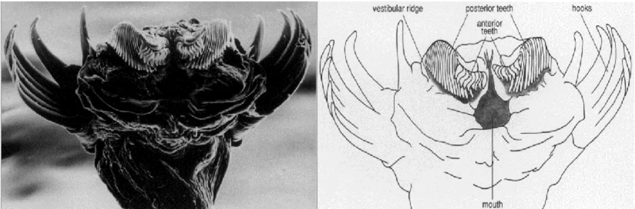
Zooplankton prey includes a wide range of ichthyoplankton and zooplankton, particularly copepods (e.g. Terazaki 2004). Prey is sensed mechanically; chaetognath hairs detect vibrations at distances of 1-3 mm (Feigenbaum & Reeve 1977, Goto & Yoshida 1981). Specific prey types can be differentiated by their unique movements (Tonnesson & Tiselius 2005). The eyes of chaetognaths lack lenses capable of forming images but they do contain a pigment that detects light direction (Pearre 1973). Therefore, their eyes may help them to detect prey outside the maximum distance for hair detections (Goto & Yoshida 1981). Dorso-ventral undulating movements are used to dart at prey, which is then seized by the hooks and punctured by rows of small teeth (Figure 1.7). The locomotion appendages, as well as the feeding appendages, differ between chaetognath species, for instance Eukrohnia hamata lacks anterior teeth (Furnestin 1965), present in P. elegans (Terazaki 1993). Relatively large items are consumed by expansions of the head (Bieri & Thuesen 1990). Chaetognaths may paralyze prey by secreting a bacterial-produced neural poison (tetrodotoxin) from vestibular ridges (Thuesen & Kogure 1989, Bieri & Thuesen 1990, Figure 1.7).

Figure 1.7 Photograph of a chaetognath’s head taken by Scanning Electron Microscopy

13

In the waters of Nova Scotia (Canada), Sameoto (1971, 1972) suggested that the abundant

Parasagitta elegans could remove considerable fractions of the copepod standing stock per

day (36 % to ˃100 % depending on season). Welch et al. (1992) suggested that Eukrohnia

hamata and Pseudosagitta maxima may ingest up to 51 % of the copepod biomass in

Lancaster Sound annually, but noted that their conclusions for these chaetognaths were “little better than guesses” (Welch et al. 1992). The above estimates of predation rates or proportion of prey standing stock removed, were based on observations of gut contents in dead chaetognaths, and specifically, methodology which treated visible lipid droplets in their bodies as evidence of recent prey digestion (e.g. Sameoto 1971, Sameoto 1972, Sameoto 1987). This approach was also adopted for E. hamata in the Southern Ocean (Froneman & Pakhomov 1998). Including lipids in predation rate calculations may be suitable for species without considerable capacity for lipid storage. For Eukrohnia species it seems there is a risk of confusing diagnostic lipid stores with oil droplets from copepods, which is likely to have occurred in at least the Sameoto (1987) study (Øresland 1990). Several other polar studies on E. hamata, as well as P. elegans and P. maxima, have reported much lower predation rates when lipid droplets were excluded from the estimates (e.g. Sameoto 1987, Øresland 1995, Froneman & Pakhomov 1998, Brodeur & Terazaki 1999, Bollen 2011, Giesecke & Gonzalez 2012).

Whilst chaetoganths are generally recognized as predators, several studies have also observed algae (e.g. Alvarino 1965, Boltovskoy 1981, Alvarez-Cadena 1993, Kruse et al. 2010) or high amounts of algae biomarkers (e.g. Philp 2007, Connelly et al. 2014) in chaetognath guts, possibly indicating that these opportunistic feeders also ingest algae in seawater or graze them from a substrate. Chaetognaths belonging to the genera Archeterokrohnia and

Heterokrohnia reside in the nepheloid layer, where they are reported to feed on organic

matter and bacteria from sediments (Casanova 1986). In an interesting recent study, Casanova et al. (2012) suggested facultative osmotrophy (ingestion of dissolved organic matter in ambient seawater) as the main mode of nutrition in chaetognaths.

14

1.3.6 Fatty acids and stable isotopes

Fatty acid profiles and stable isotope signals can also reveal information about consumer diets, trophic positions, as well as the main primary producers in the food web. Chaetognaths are easily stressed and damaged in plankton sampling nets. Potential food loss from damaged guts or stress-induced regurgitation and defecation, as well as cod-end feeding, can all bias gut content analyses and predation rate estimates (see Baier & Purcell 1997 and references therein). In contrast to gut contents, fatty acid and stable isotope signals can persist for weeks or months (Dalsgaard et al. 2003, Arim & Naya 2003). Fatty acid analysis is based on the premises that (a) fatty acids are produced by specific organisms, and (b) the fatty acids undergo limited breakdown and transformation in consumers (Dalsgaard et al. 2003, Arim & Naya 2003). Nitrogen isotopes are used to assess trophic position, based on the premise that the 15N/14N ratio undergoes a constant level of change between trophic levels (Minagawa & Wada 1984, Michener & Schell 1994). Previous studies have used this technique to infer that

Eukrohnia hamata may feed more omnivorously than Parasagitta elegans in the Arctic

(Søreide et al. 2006, Hop et al. 2006). Carbon isotopes can indicate the carbon source in a food web since the 13C/12C ratio differs little between a consumer and its food (Hobson & Welch 1992).

1.4 Climate change and other challenges for Arctic marine life

Over millions of years, Arctic marine ecosystems have been shaped by profound environmental changes that include transitions between glacial periods and interglacial periods, in addition to large variations in sea level (Darby et al. 2006). However, the 2-3 ºC rise in mean annual air temperatures since 1950 (Chapman & Walsh 2003) has had an anthropogenic source (greenhouse gas emissions, and CO2 in particular). Sea surface temperatures are increasing 2-3 times as fast as in the temperate oceans (known as ‘Arctic amplification’), as elevated influx of warm Atlantic waters causes major heat advection (Spielhagen et al. 2011). Overland et al. (2014) predicted further warming by up to 13 °C prior to the autumn of 2100 if greenhouse gas emissions continue unabated. Consistent with these changes, conditions in the Arctic Ocean are becoming more similar to those in temperate oceans (referred to as ‘Atlantification’, see Wassmann et al. 2006).

15

Arctic seas are acidifying twice as fast as temperate seas due to enhanced CO2 solubility in colder waters (Bates et al. 2011). This shift could directly affect zooplankters such as the pteropod mollusc Limacina helicina, a prominent component of Arctic zooplankton communities (Gannefors et al. 2005). L. helicina precipitates CaCO3 to build a shell required for its survival. However, experiments suggest that the lower pH values expected to occur by the end of the century will be associated with a drastic 28 % decrease in shell calcification rate and the death of these animals (Comeau et al. 2009).

Previous studies have reported decreases in both the annual mean extent of Arctic sea-ice by 3.5-4.1 % per decade (1979-2012; IPCC 2014), and mean sea-ice thickness at the end of the melt season by 1.6 m (1958-2000; Kwok et al. 2009) as well as a 5-day increase in the length of the summer melt-season (1979-1996; Smith 1998). Further sea-ice loss would be disastrous for species that depend on sea-ice to live, hunt and breed, such as some invertebrates and vertebrates including the polar bear. Ice algae would also lose their substrate (Loeng et al. 2005). Despite this, some phytoplankton taxa may benefit because a major barrier to sunlight access would be removed. Whilst oceanic primary production has recently decreased at lower latitudes, Pabi et al. (2008) reported an overall ~30 % Arctic increase in oceanic primary production between 1998 and 2006. Ardyna et al. (2014) also noted that phytoplankton blooms in autumn are becoming more common throughout the Arctic, as reduced ice cover allows winds to stir the water, breaking down any existing water column stratification, and making nutrients previously at depth available to phytoplankton near the surface. Another consequence of the recent sea-ice melt combined with an increased river discharge (Peterson et al. 2002) has been an increase in water column stratification (McLaughlin & Carmack 2010). This has created a scenario in which nutrients in shallow water can become more quickly depleted by its algal residents. Li et al. (2009) have already reported a corresponding shift from larger cells (i.e. diatoms) to smaller algal cells (i.e. pico-phytoplankton) which can extract available nutrients more efficiently. Such changes in the composition or biomass of primary producers could result in unpredictable ‘bottom-up’ effects that ripple through planktonic grazers to higher trophic levels. In the future, possible loss of ice algae blooms and changes in the timing of phytoplankton blooms could cause

16

more ‘mismatch’ scenarios in the development of primary producers and grazers, with consequences for entire food webs (Søreide et al. 2010, Leu et al. 2011).

Changes in zooplankton abundances may also affect the survival of consumers which selectively take larger lipid-rich taxa. Falk-Petersen et al. (2007) suggested that warming in the Barents Sea (+2-3 ºC) could result in the replacement of two large lipid-rich species of copepods (Calanus glacialis and C. hyperboreus) by a smaller, lipid-poor North Atlantic congener species (C. finmarchicus). This may adversely affect specialist feeding seabirds whilst benefiting herring and baleen whales, herring predators. Global warming is also associated with northern movements of previously southern fish and mammals. There are recent reports of northern movements of NE Atlantic Cod in the Barents Sea (e.g. Kjesbu et al. 2014) and of killer whales in the Canadian Arctic (e.g. Higdon et al. 2012). As particularly voracious predators on seals and fish, killer whales could exert top-down effects on lower trophic levels, with unpredictable effects on zooplankton (Ferguson et al. 2010).

Arctic seas provide a wide range of ecosystem services for sustenance, recreation and the well-being of people living within and outside the Arctic (e.g. petroleum products, fish, animal furs, tourist destinations). Seabed beyond the Arctic Circle is thought to contain 30 % and 13 % of the world’s undiscovered oil and gas respectively, with the majority of undiscovered oil located in Arctic Alaska (Bird et al. 2008). With ice-free waters expected to occur as early as September 2045 (Laliberté et al. 2016), these supplies will become increasingly accessible and may be exploited as global population grows. Potential oil spills are a concern because Arctic ecosystems are frail and Arctic seas present significant containment and recovery challenges. The ecological impacts of previous large spills in sub-Arctic waters have been considerable (e.g. Exxon Valdez 1989 in the Gulf of Alaska), with spilt oil persisting in marine habitats for decades after spillages (e.g. Peterson 2001). Shipping has also increased: with a change in the number of recorded vessels travelling through the Northern Sea Route from 4 in 2010 to 71 in 2013 (Linstad et al. 2016). This also exposes ecosystems to increased pollution, and so careful regulation placed on activities will be critical to maintaining Arctic biodiversity. Worldwide increases in jellyfish populations in recent years have been a concern for human health and marine operations such as fishing,