Flexible Point-Based Rendering on Mobile Devices

HAL Id: inria-00606748

https://hal.inria.fr/inria-00606748

Submitted on 22 Jul 2011

HAL is a multi-disciplinary open access

archive for the deposit and dissemination of

sci-entific research documents, whether they are

pub-lished or not. The documents may come from

teaching and research institutions in France or

L’archive ouverte pluridisciplinaire HAL, est

destinée au dépôt et à la diffusion de documents

scientifiques de niveau recherche, publiés ou non,

émanant des établissements d’enseignement et de

recherche français ou étrangers, des laboratoires

Flexible Point-Based Rendering on Mobile Devices

Florent Duguet, George Drettakis

To cite this version:

Florent Duguet, George Drettakis. Flexible Point-Based Rendering on Mobile Devices. IEEE

Com-puter Graphics and Applications, Institute of Electrical and Electronics Engineers, 2004, 24 (4),

pp.57-63. �10.1109/MCG.2004.5�. �inria-00606748�

Flexible Point-Based Rendering on Mobile Devices

Florent Duguet and George Drettakis

REVES/INRIA Sophia-Antipolis, France,

http://www-sop.inria.fr/reves

Abstract

Point-based rendering is a compact and efficient means of displaying complex geometry. Our goal is to enable flexible point-based rendering, permitting local image refinement, required for example when zooming into very complex scenes, and efficient shadow computations. We use hierarchical packed point representa-tions, based on recursive grid data structures. Such compact structures are particularly well adapted to devices with limited memory and display resolution, such as PDA’s. To achieve flexible rendering we store interme-diate attributes such as normals and colors at internal nodes of the hierarchy. We examine the memory and computation tradeoffs involved in the type of structure used, and find that tri-grids (3x3x3 hierarchical grids) are a suitable compromise for many cases. We show implementations of our method on PC and on a PDA, for octrees and tri-grids. The PDA version can render objects sampled by 1.3 million points at 2.1 frames per second.

1

Introduction

Recent years have seen the proliferation of complex virtual environments with the deployment of the more ubiquitous computer, which we now use at work, in the household, for leisure etc. With the increasing demand for detailed and high quality geometric models, typical scene size, containing for example scanned 3D objects, easily reaches millions of geometric primitives. At the same time, display devices are becoming more diverse, including mobile or embedded platforms such as personal digital assistants (PDAs) or mobile phones, thus significantly increasing the user base for complex virtual environments.

The main motivation of our work is to allow interactive display of complex scenes on different kinds of platforms with heterogeneous rendering capabilities. The traditional 3D object representation with vertices and polygons (faces), coupled with the traditional rendering pipeline are not always well suited in such a con-text. The gain of standard rasterization coherence is lost when many polygons project onto a single pixel of the screen. The visualization of such complex scenes quickly becomes challenging: models do not fit in main memory even on high performance graphics workstations. This reasoning is even more relevant for mobile plat-forms such as PDAs where screen resolutions around a hundred thousand pixels are typical (320x240), memory is quite limited, and computational capabilities are limited to integer arithmetic with simple instructions.

To accommodate all the above constraints, we choose a packed hierarchical point-based representation for rendering. Point-based rendering has gained popularity in recent years, offering a simple-to-use level of detail mechanism, since the number of points rendered can be adapted to the screen size of the underlying object. Initial work in point-based rendering concentrated on the generation [9, 6] and structuring [7] of points and rendering quality [10]. More recent work has introduced hierarchical structures for points using coding techniques, which allow very compact storage of massive models [2].

Our work strives to achieve flexible rendering, that is the ability to render only parts of the hierarchical data structure as necessary, including interior hierarchy nodes. In particular, we need to avoid the traversal of the entire hierarchy, and the reconstruction of normals/colors for interior nodes, since both can be prohibitively expensive operations. To this end, we store model attributes such as normals and color information at inter-mediate nodes of the hierarchy, allowing very efficient rendering of large models, since only a fraction of the

total number of samples is rendered. This approach also allows us to efficiently perform view-frustum culling and level of detail selection without the need to traverse the entire hierarchy. Flexible rendering also allows the traversal of the hierarchy in a specific order, resulting in a fast, one-pass shadow mapping algorithm.

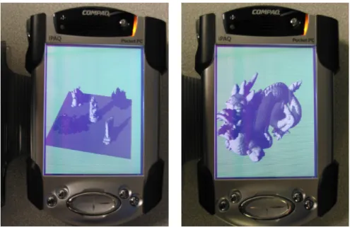
Figure 1: (Left) Our structure used for hierarchical point-based rendering of a 4.7M polygon model at 2.1 fps on a 200Mhz IPAQ, sampled at 1.3 M points total. The multi-level approach restricts the number of points rendered depending on the view. Notice the shadows in the scene. (Right) The dragon model at 2.3 fps.

The data structures we use are recursive grids. In what follows, we refer to aρxρxρrecursive grid as a

ρ-grid. Using this terminology, an octree is 2-grid, used for example by Botsch et al. [2]. The data structures used can be stored as a packed data bit stream encoding the hierarchy, both with and without the normal/color attributes. For rendering, additional pointers need to be stored in-core allowing random access to the hierarchy. We examine the storage and rendering time tradeoffs of these structures. This study indicates that for our flexible rendering approach tri-grids (3-grids), are an appropriate compromise, since they permit memory savings of about 33% for the in-core data structure used for rendering, compared to octrees. Our conclusions are backed up with experimental statistics on a set of typical models.

In the next section, we briefly present previous related work. We discuss the method of Botsch et al.[2] in some detail, since we have been inspired by some of the choices they made. We next describe our storage scheme, the various tradeoffs depending on the data structure used, and why we choose to use the tri-grid. We then discuss our flexible rendering algorithm and our fast shadow approach. Compact and efficient structures such as the tri-grid become particularly important when the geometric model does not fit in main memory, especially for mobile platforms. We have implemented our structure and rendering algorithm both on a standard PC, and on a 200Mhz Compaq iPAQ H3850 running PocketPC 2002. We present results and statistics of our method, justifying our choices, and conclude.

2

Previous Work

For very complex scenes, the traditional graphics pipeline can be wasteful, with much effort spent transforming and rasterizing large numbers of geometric primitives which may cover less than a pixel. Point based render-ing, introduced as early as 1985 by Levoy and Whitted [5], addresses this issue by point-sampling complex geometry, and rendering an appropriate number of points depending on the screen size of the complex object.

Several papers have been published in this domain over the last few years. Grossman and Dally [4] gener-ated point representations of objects in a preprocess, and presented efficient rendering algorithms of these point sets.

One approach is to generate unstructured point sets, by generating point-samples stochastically as a pre-process or procedurally on the fly [9]. Another approach is to generate structured point sets, for example by creating a hierarchy. The QSplat algorithm is such an approach permitting the visualization of very complex models [7], in particular those that do not fit in main memory. A hierarchy of bounding volumes is created, and flexible rendering is achieved by halting the descent into the hierarchy depending on rendering speed require-ments and screen size. Intermediate normal and color attributes are stored in this hierarchy. This approach was later extended to handle network transmission [8].

Pfister et al. [6] create an octree representation in their Surfels method. Surfels [6], surface splatting [10] and point-set surfaces [1] also address, among other aspects, high-quality rendering issues.

Inspired by techniques related to geometric coding [3], a more compact representation is presented by Botsch et al. [2], in which an octree is used to code point positions implicitly. This representation is based on an octree cell. If the cell hits the surface, then it is marked. All marked cells are then split up to some level. The maximal depth of the octree has to be known in advance. For each non-leaf cell of the octree, an eight bit code is stored: the childhood code. Each bit of this code corresponds to a leaf cell. The bit is set if the cell is marked. Using this technique, marked cells are stored as eight bits codes and empty cells come for free. It is important to note that sample positions are coded implicitly using this bit-code mechanism.

As a result, this approach is extremely memory efficient, and the authors present a very rapid rendering algorithm. In particular, the rendering algorithm factorizes transformations during hierarchy traversal, thus achieving very fast point projection for display. This work has inspired our approach and our choices for both storage and rendering.

The flexible rendering approach we present here combines the advantages of hierarchical and flexible ren-dering of QSplat [7, 8] and the compact and efficient storage of Botsch et al. [2]. In particular, the compact nature of the data structure allows us to store and render very complex models, enabling high-quality rendering with limited resources, and the flexibility of the approach facilitates efficient rendering.

3

Point Sampling and Storage

We next explain how we create our packed hierarchical structure, and its cost in memory. As mentioned previously, we allow flexible rendering which requires the storage of intermediate sample attributes, such as normals and colors, at interior nodes of the hierarchy. We will examine the memory tradeoffs which result from this choice. This section is dedicated to a general study of storage cost for any value ofρandσ. These values will be fixed in section 4.

3.1

Structure Creation

3D objects are often given in their traditional representation as vertices and polygons (faces). Since we need to generate our hierarchical structure from this input face set, we sample the geometry. Our sampling strategy is simple and general: for each cell of the hierarchy where geometry is present, whether interior or leaf, we sample the object at the point of the object closest to the center of the cell. If the cell hits no geometry, the cell is flagged as empty. The position of the sample point is not stored since it is implicitly given by the cell position in the hierarchy, and attributes such as normal and material index are coded using a fixed number of bits, notedσ.

In what follows we use a 16-bit code for a 13-bit quantized normal index (as in [2]) and for indexing 8 materials. Evidently, we need more bits if we have more materials or colors.

3.2

Storage Requirement Analysis

Number of non-leaf cells in aρ-grid To study the cost of our hierarchical structures, we separate the struc-ture into two parts: the hierarchy without the leaf cells and the leaf cells attributes. Depending on the chosen value ofρ, we need to compute the number of interior cells, i.e., cells that are not leaf cells. The set of leaf cells are stored in an array of sample attributes and will be the same whatever the hierarchical structure chosen. The hierarchical representation is especially well suited for grids with a small number of non-empty cells. In the typical example of a plane in space, only a small subset of the cells are not empty. For the octree, at any level, the number of non-empty subcells for an axis aligned plane is 4 = 22, while the number of subcells in an octree cell is 8 = 23. For the general case of aρ-grid, the number of non-empty subcells for a plane isρ2.

In the following, we suppose that, on average, we haveρ2non-empty subcells per non-leaf cell. As shown in the results and statistics (Section 5), this assumption is valid for many surfaces at a fine enough level.

Let n be the number of leaf samples, and k the depth (i.e., the number of subdivision levels) of the structure, then we shall haveρ2k_{= n. The number N of non-empty interior cells is thus given by:}

N = k−1

∑

Note that this number of intermediate samples in the structure depends on the number of leaf samples n and on 1/ρ2. Thus, we expect to have fewer intermediate samples for the tri-grid than for the octree.

Storage Requirement for single level rendering The efficient encoding scheme introduced by Botsch et al. [2] can be extended to generalρ-grids, usingρ3bits for each non leaf cell childhood code. The memory cost

C of this representation in bits, without the cost of intermediate samples attributes (such as normals or colors),

is the following:

C = N ∗ρ3= n − 1

ρ2_{− 1}ρ

3 ₍₂₎

The cost c0per leaf sample is thus given as (Eq. (2), (1)): c0= C n = n − 1 n ∗ ρ3 ρ2_{− 1}≈ ρ3 ρ2_{− 1} (3)

Note that the cost C accounts for the hierarchy of cells. The total cost of the structure also includes the cost of the leaf points attributes (normals/colors) which is the same whatever the hierarchical representation.

Additional storage for intermediate samples If no intermediate samples are stored in the interior nodes of the hierarchy, the entire hierarchy needs to be traversed since the leaf cell attributes need to be accessed. This can be prohibitively expensive, since traversing the hierarchy can be much more expensive than projecting and displaying a sample representing an intermediate node.

We thus store attributes (e.g., normals or colors) for intermediate samples at each interior hierarchy cell. These intermediate sample attributes are used to efficiently render a whole branch of the tree as a single sample. The cost per non-leaf cell is thus increased by the cost of an attribute: σ. The cost of an internal node is now

ρ3_{+σ. The storage cost per leaf sample c}

σis thus:

cσ=ρ

3_+σ

ρ2_{− 1} (4)

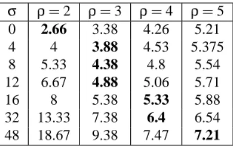
Table 1 summarizes the different costs per leaf sample for various values of ρ and σ. Note that with no intermediate attributes (σ= 0), the octree is the most memory-efficient structure, but for intermediate attributes

with size greater than 4 bits, the octree is no longer the best structure. The figures given in Table 1 are based on equation 4. Experimental results (see Table 2) confirm these figures.

σ ρ= 2 ρ= 3 ρ= 4 ρ= 5 0 2.66 3.38 4.26 5.21 4 4 3.88 4.53 5.375 8 5.33 4.38 4.8 5.54 12 6.67 4.88 5.06 5.71 16 8 5.38 5.33 5.88 32 13.33 7.38 6.4 6.54 48 18.67 9.38 7.47 7.21

Table 1: Variation ofρ-grid storage cost per leaf sample withρand the number of bits per sample attribute (σ). The bold numbers are the most efficient structure for a givenσ. σ=0 corresponds to no sample attribute, as in [2].

The structure can be stored as a bitstream: for each cell, we store the attribute, the code of child cells (zero for empty cell, and one for non-empty cell) usingρ3bits, then we store the non-empty child cells. Note that leaf sample attributes can be interleaved in the structure providing good cache coherence when accessing the bitstream.

3.3

Runtime Storage for Flexible rendering

To achieve flexible rendering, random access to the hierarchical structure is required. In particular, each cell needs to be accessed in any order.

We use the following structure to provide such flexibility: for each interior cell we store the intermediate attributes (normals and colors), and a pointer to a table of child cells. The size of the child cells table and random access to it can be obtained using the childhood code of the cell (see Section 2). This pointer to the table requires an additional 32 bits of storage per non-leaf cell. Using this approach, the traversal is completely flexible, a whole sub-branch of the tree can be skipped and child cells can be traversed in any order.

In this configuration, the memory requirement for such a structure is given Table 1 on the bottom rows. For an attribute size of 16 bits, which is the coding we use here,σis 48 (32 for the pointer and 16 for the attributes). All the tables of child cells are contiguously stored in a large table so that there is no additional cost of storage for the tables themselves. The pointer to a table can be seen as an index to the large table.

4

Flexible Rendering

We extend the rendering algorithm of Botsch et al.[2] to enable flexible rendering. We reuse the same concept of transformation factorization, but introduce a test for each cell whether it should be rendered at this level as a splat or a single point (splat condition), or whether sub-cells should be rendered. This extension can also be seen as the adaptation of the QSplat [7] rendering algorithm to this new data structure. This is possible because we can access the sub-cells independently from one another and for any level of the hierarchy. The pseudo-code is as follows:

Render (cell, center, level) if splat condition

for each subcell if sampled

compute position Draw Splat at subcenter

else

for each subcell if exists

compute subcenter

Render (subcell, subcenter, level+1)

4.1

Intermediate Node Rendering and Splats

To render intermediate nodes, we compute a conservative approximation of the projection of a cell (a cell being an axis aligned cube), and render a rectangular splat. The user selects a splat size s in pixels; in all examples presented here s is equal to 1. A larger s results in faster frame rates. We compute the screen-space bounding rectangle of the cell. This is done by computing a bounds table in a manner similar to cell centers displacements [2]. The screen-space bounds are given as (minx, miny, maxx, maxy); we also compute minz/w, which is the minimum homogeneous depth of the bounding box. See Figure 2 for different values of the splat size.

For each level, if the extent of the projected cell bounding box is less than the splat size (or a pixel), we draw the intermediate sample. As with previous point-based approaches we render rectangular splats to represent these samples. Denote dx = (maxx− minx) the extent in x and s the splat size.

The test to determine whether we stop at this level is performed in homogeneous coordinates for each dimension (dx and dy), which costs two multiplications and two tests, as shown next:

dx

w ≤ s, w > 0 (5)

which is equivalent to

dx ≤ ws, w > 0 (6)

This flexible rendering also permits view-frustum culling. If the conservative projection of the cell is out of the screen bounds, or the cell is completely behind the viewer, then the cell is not rendered at all.

4.2

Shadows

Our approach is well adapted to efficient shadow map computation. If we use the standard shadow-map algo-rithm, for each pixel of the image (with depth), we transform to the light source coordinate system using a 3x3 matrix. This operation requires 9 multiplications, 6 additions, and a test in the shadow map per pixel, without shading. For a typical iPAQ screen, this step would require 690,000 multiplies, and 540,000 additions or tests. For directional light sources, we can modify our flexible rendering algorithm to compute shadows in a single pass. Given the light direction, we can use a strict ordering in the rendering of the hierarchical structure. As shown in Figure 3, we can define an ordering on subcells so that cells are rendered in front to back order. This idea has been proposed for the depth buffer by Botsch et al. [2], but could not be implemented using their rendering algorithm, as the authors mention.

This ordering is precomputed once for theρ3_{sub-cells for a given light source direction by projecting} subcell centers along this direction. By traversing the hierarchy in this order, we guarantee that lit samples are rendered first, and samples in shadow are rendered afterwards. Thus, we compute the shadow map and the view from the camera at the same time, and perform the depth comparisons as we render. Note that computing both positions requires an additional displacement table, and an additional temporary position.

Figure 2: Using splats for rendering. Left, two pixels splats, Right, five pixels splats. 1 2 3 4 5 6 7

Figure 3: Ordering for shadow map rendering.

With this technique, we avoid the expensive matrix multiplication for each pixel of the screen and interleave the rendering from the light source and rendering from the viewpoint into a single pass. This also results in better cache coherence. The performances of this one-pass approach are given in Table 3.

It is important to note that these algorithms (multi-level, splatting and shadows) are given for generalρ -grids and could be applied to any specific type of grid, the octree being one of them. Our choice of the tri-grid for both storage and rendering is justified by Tables 1 and 3. The tri-grid is more efficient than the octree in memory consumption when storing intermediate attributes. From Table 1, 4 or 5-grids may seem more appropriate. The drawback of these structures however is the fact that the “jump” between levels becomes problematic since an interior cell is replaced by 64 or 125 children resulting in a large amount of overdraw, and in very visible popping artifacts if the splat size is more than one pixel. Different grid types could be used within the same runtime environment with a minimal overhead. The valueρ= 3 has given good results both in

terms of runtime storage (σ= 48), and in terms of rendering quality/performances.

5

Implementation and Results

In this section we present the results of our data structure construction and point-based rendering. The tri-grids and octrees are computed on a workstation, and transferred to the iPAQ. The iPAQ we use has a 200Mhz processor with 64 Megabytes of main memory. In practice however we have about 8-9 Mbytes available for our data structure, with the graphics mode enabled.

Figure 4: (Left) The “Big” (see Table 3) scene rendered on the iPAQ. (Right) The Lucy model rendered as a 2048x2048 image with level 7 of the tri-grid on a PC (53 million points).

tree models. All statistics are for 16 bit attribute samples, that is 13 bits for normals and 3 bits for a material index (but this layout is not restrictive). The disk storage requirements are close to the ones expected (σ= 16),

as well as the run-time storage requirements (σ= 16 + 32 = 48). We also implemented the algorithm on a PC

using floating point arithmetic and fixed-point arithmetic. All implementations are in C++. We have included an electronic version of a movie showing our system in use on the PDA1_.

5.1

Implementation issues

Most mobile platforms do not have floating point units. As a result direct porting of graphics code will have significantly reduced performance. In addition, certain complex instructions may not be implemented; for example a division can be more expensive than a look-up in a precomputed table. This was confirmed on the platform we use.

We implemented fixed point arithmetic for the purpose of our renderer, i.e., multiplications and additions. We also implemented an approximation of the inverse up to a given precision using a look-up table. Since we use 32-bit fixed point numbers, a global look-up table could not be used. We use a shift on numbers instead, with table size depending on expected precision.

Note that even on platforms equipped with FPUs, rendering is more efficient using fixed-point arithmetic rather than floating-point arithmetic. This is due to the final conversion from screen coordinates in floats to array indices as integers. This final step is a simple shift with fixed-point values, but is more expensive in floating-point.

5.2

Basic Statistics

In Table 2 we present a set of statistics on memory usage of our data structures. The basic statistics for the three main data structures are shown. We show statistics for two levels of both the octree and the tri-grid, for a set

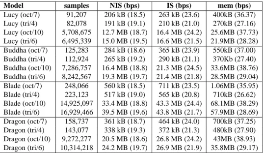
Model samples NIS (bps) IS (bps) mem (bps) Lucy (oct/7) 91,207 206 kB (18.5) 263 kB (23.6) 400kB (36.37) Lucy (tri/4) 82,078 191 kB (19.1) 210 kB (21.0) 270kB (27.16) Lucy (oct/10) 5,708,675 12.7 MB (18.7) 16.4 MB (24.2) 25.6MB (37.73) Lucy (tri/6) 6,495,339 15.0 MB (19.5) 16.6 MB (21.5) 21.9MB (28.28) Buddha (oct/7) 125,283 284 kB (18.6) 365 kB (23.9) 550kB (37.00) Buddha (tri/4) 112,924 265 kB (19.2) 290 kB (21.1) 370Kb (27.40) Buddha (oct/10) 7,286,757 16.4 MB (18.8) 21.3 MB (24.5) 33.6MB (38.76) Buddha (tri/6) 8,242,567 19.3 MB (19.7) 21.4 MB (21.8) 28.5MB (29.04) Blade (oct/7) 248,066 560 kB (18.5) 711 kB (23.5) 1.06MB (35.95) Blade (tri/4) 223,123 517 kB (19.0) 565 kB (20.8) 710kB (26.62) Blade (oct/10) 14,925,097 33.4 MB (18.8) 43.3 MB (24.4) 68.1MB (38.29) Blade (tri/6) 16,929,466 39.5 MB (19.6) 43.8 MB (21.7) 57.9MB (28.69) Dragon (oct/7) 158,737 361 kB (18.7) 464 kB (24.0) 700kB (37.25) Dragon (tri/4) 143,077 338 kB (19.3) 372 kB (21.3) 480kB (27.90) Dragon (oct/10) 9,272,277 20.5 MB (18.6) 26.8 MB (24.2) 43MB (38.93) Dragon (tri/6) 10,314,218 24.2 MB (19.7) 26.9 MB (21.9) 35.8MB (29.17)

Table 2: Basic statistics. The results are presented for the octree at level 7 (oct/7) and level 10 (oct/10), and for the trigrid at level 4 (tri/4) and 6 (tri/6). Samples: the number of leaf samples; NIS: bytes on disk without intermediate attributes; IS: bytes on disk with intermediate samples; Mem: size of in-core structure including pointers and intermediate samples. For all columns, bits per leaf sample are shown in parenthesis.

of models. The structures are evidently different; however we have chosen subdivision levels which are more or less equivalent for each. For example, 4 levels of subdivision for the tri-grid of the dragon model results in 143,077 samples, and 7 levels of the octree in 158,737. These subdivision levels gives structures which can fit in the memory of the iPAQ we used in our experiments. Subdivision level 10 for the octree and 6 for the tri-grid are used in the same manner for visualization on a PC.

We show both memory usage in megabytes, and bits per sample in parentheses. We first show statistics for the recursive grid structure without intermediate attributes (NIS), which cannot be used for flexible rendering. In this case, the octree (which is the same as [2]) is on average 4% more efficient than the trigrid in terms of bits used per sample. However, once intermediate attributes are introduced (IS), permitting flexible rendering, the tri-grid is on average 12% more efficient in terms of memory. These numbers confirm the predictions presented in Table 1. A final compression pass using general purpose compression schemes (such as gzip) can be used. However, the compression results were inconsistent from one model to the other and from one level to the next. More interestingly, we also examine the memory usage of the structure when we include the additional pointers required at runtime for flexible rendering; the octree requires 33% more memory per sample, which is significant.

This packed hierarchical representation also permits visualization of huge geometries with a reasonable number of samples; such as the Lucy model from the Stanford Michelangelo project. This model originally contains more than 28 million triangles that do not fit in main memory, and is stored in a tri-grid at level 7 with more than 53 million point samples and attributes, for around 215 MB of RAM. This multi-level data structure permits an efficient storage of the geometry with a small approximation error (1.5x10−4_{) of the entire model in} memory. The data structure is constructed level-by-level in an out-of-core preprocessing step.

5.3

Rendering Performance and Shadows

In Table 3 we show statistics for our rendering algorithm using the tri-grid structure. The statistics are average frames per second on the iPAQ. An example of the kind of view chosen is shown in the top row (“far view”) of Fig. 5. As expected, overall rendering all of the points is more expensive than the multi-level display, especially

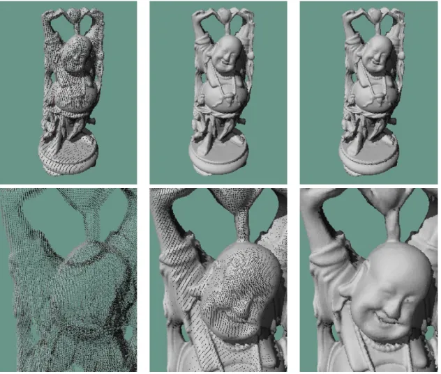
Figure 5: Above, a far view of the Buddha model shown (left) with points at level 4 (4.15 (frames per second (fps)) (middle) with points at level 5 and (0.63 fps) (right) with splats at level 5 (2.85 fps). Below, a close view of the Buddha model shown (left) with points at level 4 (4.15 fps) (middle) with points at level 5 and (0.63 fps) (right) with splats at level 5 (1.42 fps). Undersampling problems are evident at level 4 subdivision when using points only. At level 5, the increase in frame rate is significant. All fps on the iPAQ.

at maximum subdivision level 5. Nonetheless, for level 4 subdivision, the expense of computing the splats can outweigh the gain from multi-level rendering (Buddha(4) and Blade(4) in Table 3). Note, however, (Fig. 5 upper left) that Buddha at level 4 has visible undersampling artifacts with pure point rendering.

In Fig. 5, we show the problem of undersampling for a close view of a model, which is solved using splats. In addition, we show the effect on frame rate of multi-level display. Recall that multi-level display is possible because we store intermediate samples.

In the case of our largest model (Lucy), we run two versions of the rendering algorithm: flexible and not flexible for level 7 of the tri-grid with more than 53 million samples, on a window size of 512x512. The non-flexible version renders an image in around 4 seconds, and the non-flexible version for a splat size of one pixel and shadows renders 7.9 frames per second, on a Pentium IV Xeon 2.0 Ghz PC under Windows 2000.

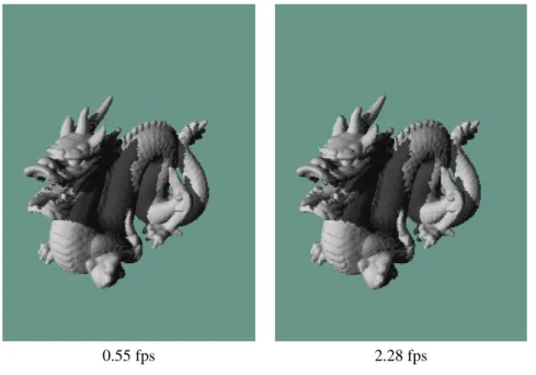
0.55 fps 2.28 fps

Figure 6: Quality and speed of shadows. View of the Dragon model shown (left) with points at level 5 with shadows and (right) multi-level display with one-pass shadows multi-level. Notice that shadows generated with multi-level rendering are practically indistinguishable from shadows generated with full point resolution.

Model Points Splats Shadows

Buddha (4) 5.49 3.47 2.99

Buddha (5) 0.91 3.33 2.85

Blade (4) 4.71 2.63 2.32

Blade (5) 0.67 2.40 2.21

Big Scene 0.62 2.38 2.11

Table 3: Statistics for our rendering algorithm (in frames per second). “Points" corresponds to direct display of points, “Splats" refers to the flexible rendering algorithm with splatting, and “Shadows" to the one-pass shadow algorithm.

6

Conclusion

In this paper we have presented a general framework for point-based sampling of complex models, which we callρ-grids. We have performed analysis of the storage requirements of these structures, and we have shown that the tri-grid is the most memory efficient when we store sample attributes for intermediate nodes.

We have used the tri-grid structure for efficient rendering of very complex models on mobile devices with limited computation and memory capabilities and a small display. We have introduced a flexible multi-level rendering algorithm which allows efficient rendering when zooming into the model, and an efficient one-pass shadow mapping algorithm. Our implementation on a 200 Mhz Compaq iPAQ PDA allows the display of 1.3M point-based representation of a 4.7 million polygon model at 2.1 frames per second.

In future work, we will be examining better reconstruction algorithms, and a progressive transmission ap-proach which will take into account network parameters. We will also investigate hybrid rendering combining different representations such as polygons, lines and points, taking into account the specific constraints of the different platforms we consider. Also, in the case of manifold objects, adaptive sampling based on surface curvature could be investigated. This might result in better compression and rendering for such objects.

7

Acknowledgements

The authors wish to thank Alexandre Olivier-Magnon for modelling the tree, using Maya, thanks to a donation of Alias|Wavefront. The Buddha, Bunny, Blade, Dragon and Lucy models are from the the Stanford 3D Scan-ning Repository http://graphics.stanford.edu/data/3Dscanrep. Thanks to Marc Stamminger and Frédo Durand for their insightful comments on an early draft.

References

[1] M. Alexa, J. Behr, D. Cohen-Or, S. Fleishman, D. Levin, and C. T. Silva. Point set surfaces. In

Proceed-ings of IEEE Visualization 2001, pages 21–28, 2001.

[2] M. Botsch, A. Wiratanaya, and L. Kobbelt. Efficient high quality rendering of point sampled geometry. In Rendering Techniques 2002, 12th Eurographics workshop on Rendering. Springer Verlag, 2002. [3] O. Devillers and P.-M. Gandoin. Geometric compression for interactive transmission. In Proceedings of

IEEE Visualization 2000, pages 319–326, 2000.

[4] J. P. Grossman and W. J. Dally. Point sample rendering. In Rendering Techniques ’98, EG workshop on rendering, pages 181–192. Springer-Verlag, 1998.

[5] M. Levoy and T. Whitted. The use of points as display primitives. Technical Report TR 85-022, Univ. of North Carolina at Chapel Hill, 1985.

[6] Hanspeter Pfister, Matthias Zwicker, Jeroen van Baar, and Markus Gross. Surfels: surface elements as rendering primitives. In Proceedings of the 27th annual conference on Computer graphics and interactive

techniques, pages 335–342. ACM Press/Addison-Wesley Publishing Co., 2000.

[7] S. Rusinkiewicz and M. Levoy. Qsplat: a multiresolution point rendering system for large meshes. In

Proceedings of the 27th annual conference on Computer graphics and interactive techniques, pages 343–

352. ACM Press/Addison-Wesley Publishing Co., 2000.

[8] S. Rusinkiewicz and M. Levoy. Streaming qsplat: a viewer for networked visualization of large. In

Proceedings of the 2001 symposium on Interactive 3D graphics, pages 63–68. ACM Press, 2001.

[9] M. Stamminger and G. Drettakis. Interactive sampling and rendering for complex and procedural geom-etry. In K. Myskowski and S. Gortler, editors, Rendering Techniques 2001, 12th Eurographics workshop on Rendering. Eurographics, Springer Verlag, 2001.

[10] M. Zwicker, H. Pfister, J. van Baar, and M. Gross. Surface splatting. In Proceedings of the 28th annual