Multi-criteria optimization algorithms for high dose rate brachytherapy
130
0
0
Texte intégral
Figure
![Figure 0.1 – The direct and indirect effects of photon beams on DNA, image from [3].](https://thumb-eu.123doks.com/thumbv2/123doknet/3204570.91599/21.918.245.674.102.482/figure-direct-indirect-effects-photon-beams-dna-image.webp)
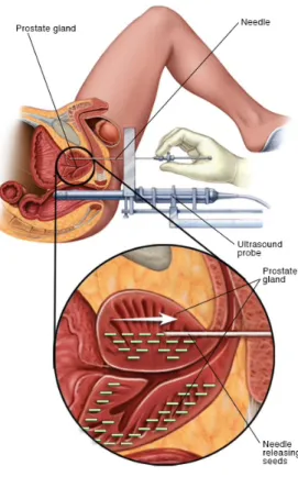
![Figure 0.5 – Treatment setups for prostate brachytherapy in the OR, images from [10].](https://thumb-eu.123doks.com/thumbv2/123doknet/3204570.91599/25.918.153.768.285.549/figure-treatment-setups-prostate-brachytherapy-images.webp)
+7
![Figure 0.7 – The electromagnetic spectrum in medical imaging modalities, image from [13].](https://thumb-eu.123doks.com/thumbv2/123doknet/3204570.91599/27.918.144.773.113.541/figure-electromagnetic-spectrum-medical-imaging-modalities-image.webp)
![Figure 0.12 – Moore’s Law: the number of transistors per chip doubles about every two years, image from [44].](https://thumb-eu.123doks.com/thumbv2/123doknet/3204570.91599/35.918.223.682.456.900/figure-moore-law-number-transistors-doubles-years-image.webp)
Documents relatifs