OATAO is an open access repository that collects the work of Toulouse
researchers and makes it freely available over the web where possible
Any correspondence concerning this service should be sent
to the repository administrator:
[email protected]
This is an author’s version published in: http://oatao.univ-toulouse.fr/20415
To cite this version:
Chazara, Philippe
and Negny, Stéphane
and Montastruc, Ludovic
Quantitative
method to assess the number of jobs created by production systems: Application to
multi-criteria decision analysis for sustainable biomass supply chain. (2017)
Sustainable Production and Consumption, 12. 134-154. ISSN 2352-5509
Official URL:
http://doi.org/10.1016/j.spc.2017.07.002
Quantitative method to assess the number of jobs
created by production systems: Application to
multi-criteria decision analysis for sustainable
biomass supply chain
Philippe Chazara
*
, Stéphane Negny, Ludovic Montastruc
Universite de Toulouse, Laboratoire de Genie Chimique UMR CNRS/INPT/UPS 5503, BP 34038, 4 allee Emile Monso, 31030 Toulouse Cedex 4, France
A B S T R A C T
Currently, the implementation of a new production system needs to satisfy three dimensions of sustainability, i.e., it must be economically viable, socially beneficial and have a low environmental impact. Unfortunately, for the social aspect, there is a lack of theoretical underpinnings, in contrast to the environmental dimension, for which the theoretical underpinnings were studied twenty years ago. Indeed, there is not a clear common frame for the social dimension, probably due to the complexity and diversity of social issues. Furthermore, some indicators are difficult to assess because of their qualitative and subjective nature. The availability of input data to evaluate social indicators is often another major bottleneck. However, when considering a new industrial activity, perhaps the most important key indicator in the social assessment is the accrued employment generated. Indeed, the implementation of new industrial activity has the potential to promote the local economy and regional development, especially in rural areas. For authorities and the public, accrued employment is pivotal to facilitate acceptability and to ensure regional sustainability.
In this article, the authors propose a method to estimate the total number of jobs created by the development of a new activity. The classic classification of direct, indirect and induced jobs is used. The new methods are based on economic data and, more precisely, on the added value and earnings before interest, tax, depreciation, and amortization to create a correlation to estimate manpower. Different mathematical methods are used to determine the values of the correlation parameters. After comparing the different approaches, this article presents the capabilities of this evaluation and its interest for multi-criteria analysis based on a case study of the optimal design of a bioethanol supply chain in France.
Keywords: Social assessment; Jobs creation; Forecasting; Multi-criteria optimization; Supply chain
1.
Introduction
Sustainability is a crucial parameter for industrialist decision makers for the acceptance of a new business
activity. A large number of indicators have been proposed to assess sustainability, with a well-established classification into three categories: economic, environmental, and social. Simultaneously improving the three pillars of sustainability
is often perceived as a complex task since it must satisfy conflicting objectives. For example, an improvement of the environmental impact is often considered as a burden that requires an increase in cost to improve equipment quality or security or to treat outlet streams. Similarly, enhancement of the social impact can result in increased costs; however, there is not always a negative correlation between the three dimensions, for example Murphy(2002) highlights a positive relation between environmental and economic sustainability. Indeed, the relation, which seems contradictory at first sight, can be a source of progress and innovation, for example, the new devices invented by the domain of process intensification in chemical engineering. This type of equipment can have a positive effect on both the environmental and economic impacts or on both economic and social impacts.
Historically, the main criterion for decision makers was economic performance, which explains why the assessment of economic performance is now well established with proven methods. However, with the rise of environmental concerns, the environmental impact has been integrated into the list of criteria. The environmental impact has become increasingly important, and it can prevent the realization of a new project if the impact is deemed excessive. While the approaches to evaluate environmental impact maturing, the environmental impact is always more difficult to assess than the economic impact. It remains difficult to draw clear conclusions from such assessment mainly due to uncertainty but also due to the sensitivity of the results to the weight of the different con-tributions. More recently, the social contribution was included in the scope of impacts to consider by decision makers. Indeed, in this evolution, social impact plays a key role in public acceptability on the one hand and in promoting local development on the other hand, for instance, through the influence of this new industrial activity on the local economy. While the goal of our approach is to propose a multicriteria decision method for the design (or evaluation) of production systems, this paper is focused on improving the evaluation of the social impact and, more specifically, one of its metrics. Currently, there are several reasons to evaluate social impact, for example, to reduce social problems for a company with good social knowledge of all chain flow (Bérubé, 2013). Additionally, markets are increasingly concerned about the social footprint of a product or a company (Houdin, 2012). Consumers have to be aware of their choices and their impacts on the environment and social economy (Benoît and Mazijn, 2009). Finally, the United Nations Environment Program recognized a need for a task force on the integration of social criteria into life-cycle assessment (LCA) (Benoît et al., 2010). Social LCA is a tool to assess the social im-pact of a product throughout its life cycle (APESA, 2012; Sanchez Ramirez and Petti, 2011). One of the aims of social LCA is to allow companies to evaluate the social impacts on people during the life cycle of their products (Dreyer et al., 2006). Unfortunately, as Yuan (2012) observes in the domain of construction waste management, the majority of research efforts has focused on economic and environmental impacts, and they have failed to include the social impact. In the same study, the author gives three major reasons to explain the lack of investigation of social aspects: (i) the social performance is of lower priority than the time and cost objectives, (ii) the assessment of social impact is dif-ficult because many indicators are qualitative and are not always amenable to empirical measurement, and (iii) the influential stakeholders are more focused on assessing and
monitoring economic performance. However, in recent years, there has been a slow shift, with numerous studies aiming to introduce social concerns into their decision framework, for instance Brent and Labuschagne (2006), Labuschagne and Brent (2008), Caniato et al. (2014), Korucu and Erdagi (2012), Yuan (2012) and Santoyo-Castelazo and Azapagic (2014). Dreyer et al.(2010) propose a multi-criteria assess-ment of social impact focused on fundaassess-mental labor rights, and Simas and Pacca(2014) present an index to estimate employment based on production. While the development of indicators and metrics of social sustainability has been improved in recent research (ˇCuˇcek et al., 2012), most metrics remain based on qualitative or semi-qualitative data ( Benoît-Norris et al., 2011) and are consequently difficult to assess. As a result, there is a need for practical methods and tools that include the social dimension in their decision framework. Thus, the first goal of this contribution is to improve the evaluation of the social impact that a new industrial activity can have on society and, more specifically, on the expected local economic growth. As aforementioned, numerous social categories define social sustainability as a consequence; this article focuses on a specific indicator and avoids subjectivity by focusing on quantitative evaluation. When considering a new industrial activity, perhaps the most important key indicator for social assessment is the accrued employment generated. Indeed, new industrial activity implementation has the potential to promote the local economy and regional development, especially in rural areas. For authorities and the public, accrued employment generated is pivotal to facilitate public acceptability and to ensure regional sustainability. Moreover, the total number of jobs created by an industrial activity, which is one of the key cornerstones of social sus-tainability, especially in the current global context, has rarely been addressed in detail to the best of our knowledge. This social indicator is seldom included in methodologies, even if there is a general recognized agreement to integrate it to raise the level of maturity of the social assessment framework. Currently, the jobs and economic development impact model, which relies on an input–output multiplier and consumption patterns, is commonly used to assess the total number of jobs (You et al., 2012b; New Renewable Energy Laboratory, 2015). Despite great progress in the evaluation of this crite-rion, the precision of the method is questionable because of the use of a ratio, especially since the likelihood interval is not given. Furthermore, the link between the different categories of jobs is not obvious and not clearly expressed (and the data for evaluation are only available in the United States). Therefore, this paper expands upon previous research to fill these gaps. The aims of this contribution are to:
• propose an assessment method to calculate the total number of jobs created by a new industrial activity while limiting uncertainty to avoid the flaws of the environmental impact assessment.
• propose a simple and reliable method that can be used as an objective function in production system synthesis and design or as an offline tool for social assessment.
• develop metrics that are easy to compute with a small amount of quantitative data but which remain compat-ible with other sustainability metrics.
Concerning the first point, as for the environmental di-mension, the results of the evaluation of the number of jobs
created can be affected by several sources of uncertainty due to method choices, assumptions, assessment method, and data quality. It is necessary to estimate the extent of the above uncertainties to be aware of the reliability and representativeness of the obtained results. Consequently, an-other contribution of this paper is that sensitivity analysis is performed to estimate the effects of some uncertainties. To the best of our knowledge, this type of analysis has never been performed for the studied metric. Concerning the last two points, Martín(2016) highlights that one major difficulty in using the indicators developed to evaluate each dimension of sustainability in the design of production systems is the complexity of the mathematical problems, consisting of large multi-objective optimization problems, and the fact that the objectives are not aligned.
The remainder of this paper is organized as follows. In the next section, the different criteria used to assess an activity are discussed, and the metrics to be included within our sustainability evaluation method, compatible with the multi-objective optimization problems, are presented. Section 3 depicts the different categories of jobs created and a literature review on how to assess them. The novel method to evaluate the number of direct jobs created by a new industrial activity is detailed in Section4. In Section5the formulae to assess the different categories of jobs are detailed. Before drawing conclusions, in Section6, a case study on a biomass supply chain is presented to briefly demonstrate the capabilities of this evaluation method and its interest for the multi-criteria analysis of an industrial project. In the case study, sensitivity analysis is performed after the main sources of uncertainty are identified.
2.
Discussion of metrics
A decision maker can use the three dimensions of sus-tainability to estimate the feasibility of a new project or a new activity. However, two difficulties are associated with the sustainability criteria: how to assess them and how to define whether the assessment is available. The economic criterion is the oldest and has the advantage of being based on money as the fundamental unit. The other two criteria are more difficult to define and to estimate. In the following section, the three criteria are briefly described.
2.1. Economic dimension
The evaluation of economic impact is well established. To assess economic performance, two categories of cost are considered: operating costs and investment costs. However, the estimation of risk in the investment cost is not easy and depends on the context and on the decision makers.
As a consequence, it is possible to distinguish two types of economic indicators: those that describe company operations and those that describe company viability (Arcimoles, 2012). The first set of indicators provides information about the daily operation of the company. These types of indicator are classified as microeconomic indicators and are used for the daily management of the plant: raw material consumption, inventions management, utility consumption, administra-tive expenses, wage bill, and maintenance. These indicators are important for making decisions about production and some short-term strategic decisions. On the other hand, the macroeconomic criteria, i.e., the second set of indicators, provide information about the interest of the investment and
support the decision makers when assessing the investment required, the potential profit and the economic risk. For this set of indicators, the project as a whole is considered; the most commonly used indicators are:
• Initial investment (Jansen, 1992; Peters et al., 2004; Sinnott, 2009).
• Net present value (NPV) (Arcimoles, 2012). • Internal rate of return (IRR).
• Payback period (Arcimoles, 2012).
2.2. Environmental dimension
The environmental criterion aims to estimate the im-pact of human activities on the environment. An environ-mental indicator represents a global indicator to measure the negative impact of human activity with respect to the Earth (Vogtländer, 2011b). The impact or footprint on the environment can be divided into different categories, as ex-plained by ˇCuˇcek et al.(2012): carbon footprint, water foot-print, energy footfoot-print, emission footfoot-print, nitrogen footfoot-print, land footprint, and biodiversity footprint.
The environmental criteria are more difficult to assess than the economic criteria because the estimation is not easy or well defined. Indeed, the results of such and assessment are often subject to interpretation due to the relative weights of the various contributions and the various uncertainties. There are several methods to assess the weights, however, they are based on a listing of flow exchanges between the activity and the environment. Among these methods, the traditional life-cycle assessment is widely accepted. Martín (2016) lists various approaches to estimate environmental im-pact. The assessment requires deep knowledge of the activity. The method used for this part is the life-cycle inventory (LCI), which is based on a listing of input and output flows of the studied activity and the resulting emissions (Vogtländer, 2011b).
Another method is the Eco-Cost indicator and its esti-mation, which is considered to be an easy way to perform environmental life-cycle assessment (Vogtländer, 2010). The main idea of the Eco-Cost method and its main difference with traditional LCA is that it does not list elements but tries to perform estimation of the investment in ecological equipment necessary to compensate the environmental bur-den (Vogtländer, 2010, 2011b, 2011a). This method can be decomposed into four steps: define the limit and the target of the study; quantify the incoming and outgoing flows; enter the data in a spreadsheet, and interpret the result ( Vogtlän-der, 2010).
The main advantage is that it assesses the environmental impact of economic values, which enables grouping into global scores. For our case study, this advantage is crucial be-cause for supply chain design, a common monetary basis for economic and environmental metrics avoids supplementary complexity in the formulation and resolution of large-scale multi-objective optimization mathematical model. However, some information is lost, such as the origins of the en-vironmental impacts and their quantities. Therefore, this method is interesting when a global evaluation is required but questionable when analysis or improvement of an activity is sought.
2.3. Social dimension
Social life-cycle assessment is, similar to environmental LCA, focused on the impact of an activity on the social environment. The social impact can be defined as the impact on worker lifestyle, working environment, and worker health, as well as the impact on the population.
For example, for Kafa et al. (2013) social LCA can take into account the commitment of the enterprise, customer satisfaction and the performance of workers. For Santoyo-Castelazo and Azapagic(2014), social indicators are grouped into four categories: security and diversity of supply, public acceptability, health and safety, and intergenerational issues. Different criteria are considered in a social LCA. Dreyer et al. (2006) quote some social policies for the social LCA from some companies: job creation, local/national recruitment, genera-tion of employment and technology development, stimula-tion of economic growth in developing countries, stability of employment, skill formation and development, wages, benefits and working conditions.
Brent and Labuschagne(2006) introduce a social sustain-ability criteria framework composed of 29 criteria aggregated into four major categories: internal human resources (em-ployment opportunities, equity, labor sources), external popu-lation (health, education, security), macro social performance (economic welfare, legislation), and stakeholder participation (information provisioning, stakeholder influence). To account for social issues related to nuclear power generation, Stam-ford and Azapagic(2011) retain the following eight categories of indicators: provision of employment, human health im-pact, large accident risk, local community imim-pact, human rights and corruption, energy security, nuclear proliferation, and inter-generational equity. More recently, ˇCuˇcek et al. (2012) identify eight social footprints with some discrepancies with the previous ones: human rights, corruption, poverty, online social, job, (vi) work environmental, food to energy, and health. Santoyo-Castelazo and Azapagic(2014) add security and diversity of supply and public acceptability. The first comment on these indicators is that there is overlap with the economic and environmental indicators; indeed, some impacts can be included in different dimensions of sustain-ability. For instance, human health could be alternatively assigned to both social and environmental dimensions. Based on this ascertainment, the European project Prosuite (Blok et al., 2013) has developed a framework that limits the overlap, and which is composed of five major impact categories: health, social well-being, prosperity, natural environment, and exhaustive resources. According to Houdin (2012), the most commonly used social impact indicators are Houdin (2012): human rights, health, security, governance, working conditions, economic and social repercussion, and cultural heritage. The list of social indicators used in the scientific literature is far from exhaustive, which is not the purpose here, but the provided examples lead to several comments:
• Unlike economic and environmental indicators, there is not a clear common frame for social indicators. This lack of a framework is probably due to the complexity and diversity of social issues, which depend on the type of activity or on the sector of application. There is a lack of theoretical underpinnings, in contrast to those established for the environmental dimension twenty years ago.
• As highlighted by the Prosuite project (Blok et al., 2013), social indicators are complex. Indeed, for the environmental impact, each indicator is minimized, and its magnitude is related to a specific quantity. However, for social indicators, the desired direction of optimization can be different, for instance, to increase employment but to decrease poverty. The magnitude of social indicators is also more difficult to evaluate because of the multiplicity of input data required and because the data are not always available.
• Some of the indicators are difficult to assess because of their qualitative and subjective nature. For instance, with respect to human rights (or corruption) it is not always obvious how to clearly establish rights viola-tions (or to demonstrate corruption). Perret(2002) asks whether it is possible to estimate social impact without moral judgment or political views and what types of goods have to be taken into account for this estimate. • In a social approach, every improvement necessarily
has an environmental character. Some indicators, such as human health, food to energy, and safety, influence the two previous dimensions. These indicators on the border between the social and environmental dimen-sions are estimated within life-cycle assessment. Fur-thermore, this approach permits an increase in the number of quantitative evaluations.
• The availability of input data to evaluate social indi-cators is often a major bottleneck. Combined with the third point, this availability also raises the question of uncertainty in the assessment.
Following these observations, the assessment of social sustainability must address two questions: What social cri-teria must be considered in accordance with the method-ological purpose, industrial activities, and industrial sector? How can the retained criteria be quantified? Some initiatives attempt to create methods to improve this estimation. For example, the Social Hotspots Database created by Social Sustainability at New Earth (Bérubé, 2013).
3.
Estimation of the number of jobs
3.1. Problem descriptionThe objective is to assess the number of new jobs created by the new activity in all sectors impacted by this activity.
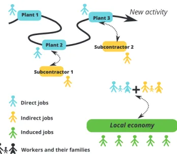
Obviously, this number is not limited to the jobs created by the new activity, for example, in a new plant, but includes the jobs created or supported by subcontractors and the local economy. The number of jobs created is a pertinent indicator to promote new activity, and it could become an attractive indicator. The total number of jobs can be broken into three sub-indicators: direct, indirect and induced jobs (Fig. 1).
The number of direct jobs created represents the total number of jobs that the activity has created directly, i.e., the hiring generated by the creation of the activity.
The number of indirect jobs is the number of subcontrac-tors working for the new activity. This number can represent new hiring or not, but it represents indirect impact on the local economy.
The last number is the induced impact on hiring in the society, which represents the employees supported by the new workers (direct or indirect) of the plant and the sub-contractors and their families in the local economy. It is the
Fig. 1 – Different types of created jobs. employment created outside the industrial activity related
to current expenditures of household consumption in the local economy due to generated employment (both direct and indirect). As a result, the total number of jobs is region specific.
3.2. Problem: how to estimate the number of direct, indirect and induced jobs
However, one of the most crucial problems is how to estimate these numbers. Moreover, the number of jobs is not a precise value but depends on assumptions based on estimates: the gross number of employees or the equivalent full-time employees. Furthermore, the type of activity is also a crucial parameter, for example, the type of process used, the size of the plant, and the production quantity. Recently, Martín(2016) proposes a method based on the in-vestment, the average salary of an employee in a region and a job multiplier coefficient to estimate the total number of jobs created. In this study, the direct jobs created by a chemical factory are computed by averaging the direct jobs created per million dollars invested. The advantage of this method is that the estimation is region dependent (job multiplier and average salary). The major drawbacks are that the number of induced jobs is not precisely estimated and that it is based on the investment. However, it is not the investment but the capacity of production that determines the number of people working (the larger the production is, the larger the number of people required to operate the plant).
Moreover, Dutailly(1983) shows that the number of jobs depends on the capital invested and the type of activity. However, this number is not proportional to the capital in-vested. The ratio of the number of jobs/capital decreases with increasing capital but not in the same way for all types of activities. This result can be in opposition to the estimation of Chauvel et al. (2001). The authors propose a method to estimate the number of jobs required for a chemical plant with respect to the quantity of production and the type of process(1). N umber.of.hours.worker/day tonne.of.product =t ∗number.of.steps.in.the.process (capacity.in.tonne/day)0.78 (1) where: t =23 if discontinuous operations
t =17 if continuous operations with medium instru-mentation
t =10 if continuous operations with good instrumen-tation
t =7 if continuous operations with control line. The expected number is not linearly related to the quantity of production. Various authors propose similar methods to estimate this number (Sinnott, 1999;Peters et al., 1968;Turton et al., 1998). However, the scope of these two methods is different. In Dutailly’s method, the total number of employees is assessed irrespective of their category, whereas Chauvel’s formula is focused only on operators, i.e., the employees working directly on production activities. Therefore, the two methods illustrate the difficulty of the task and the different parameters that influence the result.
Based on this analysis, it is possible to divide the methods into two families: comparative methods that use a database to estimate the different numbers by extrapolation and sta-tistical methods, such as Dutailly’s method, which attempt to estimate these indicators with global data from statistical studies.
3.3. Direct jobs
As introduced previously, in one of the first attempts to estimate the number of jobs created by an industrial activity, Dutailly (1983) study the ratio of the number of direct jobs/capital and conclude that the ratio decreases, not linearly, as the capital cost increases but not in the same way for the entire industrial sector. This nonlinearity is due to the importance of some tasks in employment regardless of others (Simas and Pacca, 2014), which makes the analysis difficult. However, this method has the major drawback of providing a very rough estimation due to the uncertain-ties associated with such a statistical method. For chemical plants, Chauvel et al.(2001) propose a formula to estimate the number of employees who work in the production workshop. The formula integrates the level of instrumentation of the chemical process and its production capacity. The two major limitations are the scope of the method, as it is restrained
to the chemical process, and it does not allow estimation of the global number of direct jobs created because it does not calculate the number of employees outside the boundaries of the production department. In their study on the design and planning of supply chains, the model of Santibañez-Aguilar et al. (2013) considers social impact through the number of direct jobs generated by all the activities of the supply chain.Pérez-Fortes et al.(2014) propose a method to estimate the number of direct jobs created for a supply chain by counting the number of sites that have a treatment process in order to promote work places in the widest range of commu-nities. The previous studies are not entirely suitable because the total number of jobs created by an industrial activity is not limited to direct jobs.Stamford and Azapagic(2011) go deeper and approach this problem by considering the three categories of jobs created and the different phases of the life cycle of a plant, i.e., construction, operation and decommis-sioning. Unfortunately, the direct and indirect numbers of jobs are determined approximately through expert elicitation. Furthermore, the number of induced jobs is not considered in their framework because of their application. The only method available is to use a multiplier of the number of direct and indirect jobs, which leads to a very rough estimation. In the Prosuite project (Blok et al., 2013), the total regional employment is calculated with a macroeconomic model, but as the authors have shown, the two main bottlenecks are the available data on social aspects and the fact that the results remain highly explorative and can be used to find areas of interest but further analysis is required. You et al. (2012a) use an input–output multiplier analysis, where the multiplier is a ratio that estimates the total impact resulting from an initial change in economic output. This ratio takes into account some economic and regional considerations for the three different categories of employment. Despite great progress in the evaluation of this criterion, the precision of the method is questionable because the method used to calculate the multiplier and the likelihood interval are not given. Furthermore, the link between the three categories is not obvious and is not clearly expressed.
Another method is presented by El korchi and Millet (2011), whose “job creation indicator” represents the number of hours created for each activity. The indicator is multiplied by the quantity of the activity. VNF(2012) uses a ratio be-tween the number of workers and the total investment in the studied sector. This article does the same with the indirect and induced jobs, taking into account the subcontractors and the geographic location of each plant. Therefore, it does not consider the characteristics of the firm, only the investment. Consequently, this method supposes that the same invest-ment will reflect the same activity and the same manpower, which is not always satisfied. Moreover, some works present inconsistencies and a lack of clarity in the statistics (Dalton and Lewis, 2011).
In some sectors, a formula has been developed to perform the estimation based on statistics. In the article ofVNF(2012), this method is used to compare with the statistical method. By contrast, another approach requires good knowledge about the process used, for example, the method of Chauvel et al. (2001) requires information about the number of process units and the type of process.
The comparative method estimates the value of the num-ber of jobs created by comparing the project to similar previous projects. The comparative method assumes that these numbers will be similar or proportional if the activities
are more or less the same and the production and effort required are similar. The method consists in extrapolation from a known number to an expected number using the ratio between the projects’ size. The project size can be based on the cost, investment, or evaluation of the task.
A lot of limits remain in the three described methods. Statistical methods provide a very rough estimation. Addi-tionally, it is necessary to identify a category for the evaluated activity in the statistical data, for example, using the study of Dutailly. In Chauvel’s method, the limitations come from the fact that it is a global evaluation that takes into account only people working on production jobs. In comparative methods, the problem comes from the fact that it requires similar cases of the same type of activity, on the same scale, at the same time, using the same type of method and technology.
3.4. Indirect jobs
Indirect jobs represent employees working with subcon-tractors of the activity (VNF, 2012;Insee and PACA, 2005). The following formula is often used:
IndirectJobs = pCA ∗ N bW, (2)
where pCA is the part of the turnover coming from the activity studied with respect to the global turnover of the contractor and NbW is the number of subcontractor jobs.
3.5. Induced jobs
The only formula in the literature is presented in Insee (2012b). The idea of this estimate is to assume that the number of induced jobs in the local economy is proportional to the household consumption coming from employees in direct jobs and indirect jobs and their families.
InducedJobs = JIA ∗ P W LP ∗(DJ + IJ) ∗ SF
P . (3)
This formula is based on some input data: • The number of direct jobs: DJ
• The number of indirect jobs: IJ
• The average household size at the location of the activity: SF
• The size of the population: P
• The portion of local workers supported by the local population: PWLP
PWLP is the ratio corresponding to the sales coming
from household consumption to the total sales by the sector of the activity (Insee, 2012a).
• Number of jobs in the area of the study: JIA.
These parameters include local economic data to take into account the local specificities.
The problem with indirect or induced jobs is that these numbers are difficult to quantify experimentally. By contrast, direct jobs can easily be counted in a plant. However, the number of subcontractors is based not only on those em-ployed for the studied activity but also for others activities. Therefore, this number cannot be counted directly, only es-timated. In the literature, the number is defined as the ratio of turnover of subcontractors coming from the activity and the total turnover. This estimate supposes that each worker produces the same portion of turnover. In other words, there is a linear relation between workers and turnover. However, as shown by Dutailly(1983), the number of workers is not
proportional to the invested capital. Therefore, it is possible that workers and turnover are not linearly related. Similarly, the number of induced jobs is, by definition, a statistic. The evaluation makes assumptions on how each family spends their money. Therefore, the estimate is obtained as the num-ber of people in the family divided by the total numnum-ber of people in the area studied for the portion of employees supported by population consumption. Therefore, the two indicators are two estimates that are difficult to compare with real values because the real values are difficult obtain. Finally, some differences appear as a function of the scope of the study (Llera et al., 2013).
The main conclusion is that complete estimation of jobs created is difficult; despite several attempts, only rough es-timates have been obtained. As industrial activity can have positive benefits in the area in which it is implemented, and the estimate of the accrued number of jobs must consider all the dimensions. As a consequence, the categorization of direct, indirect and induced jobs is well suited. Additionally, the economic outputs seem to be the most commonly used data to quantify this indicator, especially for direct and indi-rect jobs. For induced jobs, the features of the local area are important data to include in the evaluation. For instance, for a new industrial activity, the impact on the local economy is different in rural areas and crowded cities. For the latter, the infrastructure to absorb the new population already ex-ists, whereas in the former, new industrial activity promotes stronger rural development. Furthermore, in both cases, the local household consumption habits are an important pa-rameter to consider because they can strongly influence the number of induced jobs. The goal of the next section is to propose a method to estimate this indicator by integrating the previous requirements to fill the gap left by past studies.
4.
Proposed model
4.1. ObjectivesThis section details the proposed method to estimate these indicators. To assess the accrued number of jobs, the proposed method is based on economic data because they are well-known and easy to estimate in the beginning of a project, with a maximum error of 15%. This method differs from the previously described methods because the economic data come from annual events and not from the initial investment. Therefore, one of the main advantages is the consideration of the evolution of a firm over time. The goal of this study is to provide a good estimate of employment with very minimal but relevant data.
4.2. Economical formula
Initially, the author attempted to identify databases con-taining economic and manpower data. Therefore, the author worked with three indicators:
• Sales (CA) • Value added (VA)
• Earnings before interest, tax, depreciation, and amorti-zation (EBE)
• Manpower (EFF).
The relations between each indicator, using an economical balance for companies, are summarized here:
Sales + capitalized production = Production (4) Production − external consumption = Value Added (5) Value Added + grant − wage bill − payroll tax = EBE (6)
EBE + other profits − depreciation expense
=Operating income (7)
Operating income + income − expenses = Current result (8) Current result + extraordinary income
−extraordinary expenses = Pre-tax result (9) Pre-tax result − industrial and commercial profits
−employee profit-sharing = Net income . (10) Some input data are more important than others for estimating the manpower. First, Sales are interesting because they can be easily calculated for a firm selling products: CA =
n
X
i=1
(pricei∗quantityi). (11)
The other data are also interesting for the estimation; how-ever, they result from some calculations and require more information.
4.3. Calculation assumptions
The use of the annual economic balance requires many input parameters. As a result, some assumptions must be made to link the economic data with manpower and to remove less significative data. The latter is often difficult or impossible. First, it is possible to formulate a simple relation between manpower and sales based on an average price and using these following hypotheses:
Hypothesis 1.
Sales ≈ α ∗ production (12)
and
production ≈ β ∗ M anpower. (13) These hypotheses assume that there is a linear relation between sales and production. The first hypothesis can be justified by production and the average price of the products. The second hypothesis can be justified by an averaging effect. Additional formulae are simplified because they required data that are more difficult to obtain.
From (6):
Value Added − EBE = wage bill + payroll taxe − grant. (14)
Hypothesis 2.
grant ≈ 0. (15)
And
V A − EBE ≈ W ageBill. (16)
For this hypothesis, grant is considered to be not significant relative to the wage bill or to be non-existent. Payroll tax can be included in the wage bill and is therefore proportional to the number of employees.
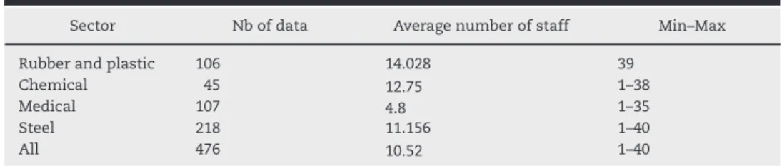
Table 1 – Number and range of data used by sectors.
Sector Nb of data Average number of staff Min–Max
Rubber and plastic 106 14.028 39
Chemical 45 12.75 1–38
Medical 107 4.8 1–35
Steel 218 11.156 1–40
All 476 10.52 1–40
Hypothesis 3.
W ageBill ≈average cost of manpower ∗ Manpower. (17) The third hypothesis assumes that there is an average manpower cost for all companies and that the wage bill depends only on the number of employees. Moreover, this hypothesis can be used to assess only the total number of jobs; we cannot obtain information about the distribution of jobs by category, i.e., engineers, operators, etc. This accurate assessment is not possible to achieve in a generic way.
4.4. Method
Three formulae are proposed to estimate manpower from economic data. Despite the strangeness of basing the study on an economic formula, correlations between economic data and social assessment have been assumed for a long time. To give an example, Preston(1975) assumes a relation between the GDP per capita and the life expectancy at birth (LEX), where α is a constant, β is a regression coefficient and ǫ is an error term:
ln LEX = α + β ln GDP + ǫ. (18) Following this approach, Feschet et al. (2012) try to create a correlation between changes in economic activities and changes in health status using the Preston pathway. Their main idea is to estimate the modification of the LEX value with an estimation of the GDP and to estimate the part of modified GDP produced by the studied activity of the national GDP to obtain the social impact of this activity.
For our study, the three correlations proposed are based on the value added (VA), the EBE and the turnover (CA):
• α ∗ CA + β ≈ M anpower
• α ∗(V A − EBE) + β ≈ Manpower • α ∗ V A − β ∗ EBE + γ ≈ M anpower.
The first formula is proposed because it is the simplest one to use. It requires only sales information. The main idea is to highlight the relation between sales, production, and manpower, if it exists. Following the same idea, the authors propose a correlation between manpower and sales similar to Thornley et al.(2008), who propose a ratio of the number of jobs created with respect to the steps and the energy production. The second and the third equations are based on the balance sheets and the hypothesis.
Additionally, two methods to find the best coefficients α and β are proposed.
The first method uses the DEPS evolutionary algorithm, with the following optimization function:
AEP =1 n n X i=1 |y − yef f |
y with y the real manpower and yeff the estimate manpower from the formula.
(19)
The second method is linear regression with the previous criterion. Then, the authors check the validity of the regres-sion according to R2, the t-value and the p-value (Pr(> |t|)).
The third method used is an artificial neural network (ANN). The advantage of ANN is that it does not require assumptions on the equations linking the input data to the output data.
4.5. Data used for the analysis
The data used here without previous treatment come from balance sheets published by French companies between 2010 and 2014. Companies in different sectors are selected to determine whether there is an impact on the estimation and whether the proposed method is generic, as shown inTable 1: rubber and plastic, chemical, medical and steel sectors.
However, there are some limitations on the conclusions from these data due to the sample size for each sector and their diversity. For example, the chemical and the rubber and plastic sectors can be considered as well-entrenched, medium-sized enterprises, the medical sector represents a new technology sector, and the steel sector is a long-term, well-established sector. This wide variety of sectors is chosen because the type of activity, and therefore the required manpower, can be vary greatly between these sectors.
4.6. First formula:α∗CA+β≈M anpower
This section estimates the manpower using only the sales information (CA). The main advantage is the ease of obtaining the input data. The results are summarized in Tables 2and3:
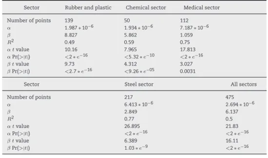
The results of the two methods are not satisfactory be-cause the AEP criterion is greater than 30% (Table 2) or because they do not have an acceptable R2 (Table 3). The
points are scattered around the estimated value, suggesting that there is not a linear relation between the sales (CA) and manpower of a company, regardless of sector Fig. 2. It is possible to conclude that there is a link, but the link is not linear due to the wide dispersion. This result can be explained in the following manner. Suppose that you have two firms,
Firm 1 and Firm 2-2, that produce the same product C with
the same quantity and the same selling price, as illustrated inFig. 3. Therefore, the sales, and consequently the number of jobs created, will be the same for the two companies. How-ever, Firm 1 produces product C using A as the raw material, and Firm 2-2 buys product B from Firm 2-1. Therefore, the activities and manpower will not be the same. In conclusion, sales, in contrast to value added, is not representative of the number of jobs. It can be used, for extrapolation, only for firms performing the same activity.
Table 2 – Results of estimating EFF with CA for the first method.
Sector Rubber and plastic Chemical sector Medical sector
Number of points 139 50 112
α 5.9017 ∗ 10−6 2.5782 ∗ 10−6 7.2207 ∗ 10−6
β 0.00114358 0.00116934 0.0011697
AEP 38% 63% 38%
Sector Steel sector All sectors
Number of points 217 475
α 7.5279 ∗ 10−6 6.1591 ∗ 10−6
β 0.000288296 0.000292573
AEP 39% 47%
Table 3 – Results of estimating EFF with CA for the second method. Sector Rubber and plastic Chemical sector Medical sector
Number of points 139 50 112 α 1.987 ∗ 10−6 1.934 ∗ 10−6 7.187 ∗ 10−6 β 8.827 5.862 1.059 R2 0.49 0.59 0.75 α tvalue 10.16 7.965 17.813 αPr(>|t|) <2 ∗ e−16 <5.32 ∗ e−10 <2 ∗ e−16 β tvalue 9.73 4.312 3.027 βPr(>|t|) <2.7 ∗ e−16 <9.26 ∗ e−05 0.0031
Sector Steel sector All sectors
Number of points 217 475 α 6.413 ∗ 10−6 2.694 ∗ 10−6 β 2.849 6.137 R2 0.77 0.5 α tvalue 26.895 21.83 αPr(>|t|) <2 ∗ e−16 <2 ∗ e−16 β tvalue 6.389 16.11 βPr(>|t|) 1.03 ∗ e−9 <2 ∗ e−16
Fig. 2 – For all sectors, the estimated values divided by the true values for the first (a) and second method (b).
4.7. Second formula:α∗(V A−EBE) +β≈M anpower This section attempts to provide an accurate estimation of manpower using the following formula:
α ∗(V A − EBE) + β ≈ Manpower. (20) The results are summarized inTables 4and5.
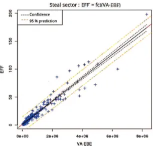
Graphs of the results obtained by linear regression are plotted in Fig. 4, and a comparison of the estimated man-power and real manman-power for the steel sector is shown in Fig. 5. The results of the other sectors are similar to those for the steel sector.
The results show that there is a linear relation between VA–EBE and EFF. However, the coefficients of linear regression
Table 4 – Results of estimating EFF with VA–EBE for the first method.
Sector Rubber and plastic Chemical sector Medical sector
Number of points 139 64 115
α 2.1744 ∗ 10−5 1.7482 ∗ 10−5 1.5288 ∗ 10−5
β 0.0002862 0.000292425 0.000292572
AEP 19.8% 33.2% 35.79%
Sector Steel sector All sectors
Number of points 255 476
α 2.0599 ∗ 10−5 1.946 ∗ 10−5
β 0.000292572 7.3145 ∗ 10−5
AEP 28.13% 31.71%
Table 5 – Results of estimating EFF with VA–EBE for the second method.
Sector Rubber and plastic Chemical sector Medical sector Number of points 139 64 115 α 2.082 ∗ 10−5 1.431 ∗ 10−5 1.816 ∗ 10−5 β 1458 2.539 4.615 R2 0.94 0.8749 0.922 α tvalue 47.24 18.127 36.110 αPr(>|t|) <2 ∗ e−16 <2 ∗ e−16 <2 ∗ e−16 β tvalue 1.641 2.495 1.451 βPr(>|t|) 0.106 0.0162 0.15 Sector Steel sector All sectors
Number of points 255 476 α 1.729 ∗ 10−5 1.903 ∗ 10−5 β 3.999 1.2409 R2 0.92 0.86 α tvalue 94.523 63.567 αPr(>|t|) <2 ∗ e−16 <2 ∗ e−16 β tvalue 7.160 6.187 βPr(>|t|) 8.42 ∗ e−12 1.17 ∗ e−9
Fig. 3 – Difference between sales and value added with respect to the activity.
are not the same for each sector, and the margin of error is approximately 30%.
The difference in the estimation of the coefficients by sec-tor indicates that the average cost of manpower is different in each sector, following the assumption. This result confirms Dutailly’s findings, which show clear differences by sector, and it seems to eliminate the possibility of a global formula. However, the estimation performed with data from all sectors is acceptable and demonstrates that a single formula can be applied in several sectors. However, a larger study must be done to confirm the result for all sectors in a country.
Moreover, although similar results, they give different co-efficients. The method based on minimizing the AEP function
Fig. 4 – Linear regression of manpower in the steel sector.
Fig. 5 – Estimation of manpower in the steel sector.
estimates the β coefficient to be zero or very close to zero, and it assumes that when the EBE approaches zero, the number of jobs also approaches zero. By contrast, the second method gives a β coefficient in the range [1;5], and it assumes that there is always employees, even if there is no production. The second assumption can be justified: if a company exists, it has at least one employee. Finally, the difference can be explained
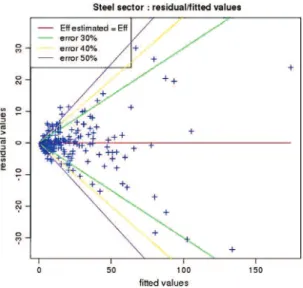
Fig. 6 – Residual values vs. fitted values of the linear regression in the steel sector.
Fig. 7 – Relative gaps for all sectors.
by the methods used: the first attempts to reduce the sum of errors between the estimated and real values, whereas the second attempts to obtain the best statistical result, even if the gap is greater.
To conclude this section, a plot of the residual values over fitted values is shown inFig. 6. The plot shows the residual values, minimizing the error in the estimation, in front of the estimated values.
Fig. 6 shows that for a major portion of the firms, the error when using this estimation formula is less than 30%. However, for companies with fewer than 25 employees, the error can exceed 50%.
Finally, Figs. 7–9 show the relative gaps between r2 =
Ef f −Ef fEstimated
Ef f and the real number of jobs (y).Fig. 7shows
that the error increases as the number of jobs tends to zero. In Fig. 8, with a focus on the interval [15, 100] employees, the plot clearly demonstrates a linear trend, as assumed. In Fig. 9, the majority of the points are between ±50%, with a concentration around zero.
In conclusion, manpower estimation is possible via linear regression using the VA and EBE data. However, the estima-tion is limited by sector and by the data set used for the linear
Fig. 8 – Relative gaps for all sectors with a staff between 15 and 100 workers.
Fig. 9 – Relative gaps for all sectors with a staff between 15 and 100 workers and where the gap is between ±50%.
regression. The error in the estimation is less than 30% for a majority of the companies, but some exceptions remain.
4.8. Third formula:α∗V A−β∗EBE+γ≈M anpower For a more precise estimate, the third formula is proposed to assign different weights to the two input data: VA and EBE. To illustrate the results, the estimated manpower over the real manpower in the plastic and rubber sector is plotted inFig. 10, and the same results for all sectors are shown in Fig. 11. For each sector, the estimated parameters and the likelihood interval are given inTable 6(orTable 7) for the first method (or second method). In the graphs, the line Bi represents Eff Estimated = Eff Real, the lines Eh2 and Eb2 indicate the interval with an error of more or less than 20% and Eh3 and Eb3 indicate the interval with error of more or less than 30%. Therefore, a majority of the points have an error of less than 20% in the plastic and rubber sector for companies with more than 20 workers, but for small companies, the error is higher. This result can be explained by the scale of the company. For example, an error of one worker in a company with only three workers represents an error of
Table 6 – Results of estimating EFF with VA–EBE for the first method.
Sector Rubber and plastic Chemical sector Medical sector
Number of points 139 50 112
α 2.07 ∗ 10−5 1.65 ∗ 10−5 1.39 ∗ 10−5
β −1.86 ∗ 10−5 −1.771 ∗ 10−5 −1.2945 ∗ 10−5
γ 0.2384 0.238 0.19
AEP 19% 31% 35%
Sector Steel sector All sectors
Number of points 217 475
α 2.10 ∗ 10−5 1.98 ∗ 10−5
β −2.35 ∗ 10−5 −1.98 ∗ 10−5
γ −0.05 0.059
AEP 30% 31.6%
Table 7 – Results of estimating EFF with VA–EBE for the second method.
Sector Rubber and plastic Chemical sector Medical sector
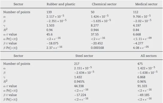
Number of points 139 50 112 α 2.117 ∗ 10−5 1.424 ∗ 10−5 9.766 ∗ 10−5 β −2.351 ∗ 10−5 −1.635 ∗ 10−5 −2.02 ∗ 10−5 γ 1.503 8.277 4.197 R2 0.94 0.944 0.84 α tvalue 45.6 37.55 6.668 αPr(>|t|) <2 ∗ e−16 <2 ∗ e−16 <1.11 ∗ e−09 β tvalue −18.075 −20.452 −4.277 βPr(>|t|) 2.37 ∗ e−16 0.000168 4.08 ∗ e−05
Sector Steel sector All sectors
Number of points 217 475 α 2.151 ∗ 10−5 1.422 ∗ 10−5 β −2.634 ∗ 10−5 −1.638 ∗ 10−5 γ 1.432 6.868 R2 0.945% 0.96% α tvalue 44.338 91.103 αPr(>|t|) <2 ∗ e−16 <2 ∗ e−16 β tvalue −17.224 −49.185 βPr(>|t|) <2 ∗ e−16 <2 ∗ e−16
over 30%, whereas the same error for a large company is less important or insignificant.
For the plot of all sectors, the estimated values show a good trend, as in the plastic and rubber sector, but they are more dispersed.
The results demonstrate a relation between manpower and VA–EBE, as found with the second formula. Moreover, the coefficients are not the same for each sector, which can be explained by the fact that there is a different degree of automation between sectors, specifically in the way in which production is managed, as explained by the results of the second formula. The same factor also explains some of the differences between firms in the same sector.
Finally, the differences between the second formula and the third formula are insignificant as the α and β coefficients are similar. For the γ coefficient, the conclusions are the same as the β coefficient of the second formula, which shows that the first method assumes that the number of jobs tends to zero when the activity is nil, and the second formula assumes that there is always employees.
4.9. Using artificial neural network
The previous sections demonstrate that there is a link between manpower and VA and EFF, which can be used for an initial estimate of the number of jobs created. However, the first formula and its unsatisfactory results indicate clearly that sales (CA) alone cannot be used for estimation via a linear function. However, in the first steps of the creation of a new activity, companies have a relevant model to quickly estimate and update the sales value to assess the economic potential of the activity and to justify its achievement. By contrast, VA and EFF are difficult to evaluate. Therefore, it is reasonable to explore the use of sales to obtain the social estimate despite the limitations. As there is not a linear rela-tion between sales and manpower, another type of relarela-tion is sought. Because the form of this relation is unknown, a neural network is proposed to estimate manpower. The advantage of an artificial neural network is its ability to learn from a set of examples to estimate a specific output from a specific input. Moreover, it is able to approximate very complex unknown functions independently of the user’s knowledge. Artificial neural networks (ANNs) are machine learning tools composed of connected neurons. Each neuron receives one or more
Fig. 10 – Estimated manpower in the plastic and rubber sector.
Fig. 11 – Estimated manpower in all sectors.
Fig. 12 – Example of feedforward multilayer perceptron.
signals and sends another signal to the other neurons. An important point is that the networks require a training period where the network will adapt its structure according to the inputs and outputs. Some ANNs are composed of slides with different numbers of neurons. One of the difficulties in the creation of an ANN is the selection of the number of slices and the number of neurons per slice. One possible technique is to create the network by trial and error, while trying to minimize the size of the network. A brute force method is commonly proposed in the literature, starting with the smallest ANN size possible. The numbers of neurons and layers are then increased to obtain the smallest ANN that provides a solution withing the targeted error range. Unfortunately, ANNs do not generate an equation.
The Neurolab library in Python is used to create and train the ANN. The feedforward multilayer perceptron, shown in Fig. 12, with the activation function TanSig is selected because it is simple to use when the behavior of the model is unknown. Two types of input are used. The first is only the turnover (CA); the second is value added (VA) and EBE. The
main aim is the same as that of linear regression, that is, to find a relation between the inputs and manpower to perform a social assessment. Then, the obtained results are compared with the results from the first method to assess the use of the ANN.
Initially, an ANN is developed to estimate the manpower of a company with VA and EBE as inputs. The error target is an average of 20%. An attempt to decrease this average is attempted, but the results after the training step are not representative. Therefore, an ANN with 20% error is selected, and it represents a good compromise.
For the training steps, 130 tuples of values are selected from all sectors. An ANN with 4 layers is identified with 2,
8, 14, 1 neurons. The target of an average error of 20% is
achieved, as illustrated in Fig. 13. For the linear regression, errors are detected for very small companies, but the results are very good for companies with more than 16 employees (represented in the plot by 40%, that is, 0.4).
To verify the ANN, it is trained with 100 different tuples, and the results are illustrated in Fig. 14. The results are acceptable because the majority of the estimated values have an error of less than 30%. However, there are some points over this limit, and the result is not better than that of linear regression. Therefore, the ANN can be used for this case, but it is difficult to train and to identify the optimal structure.
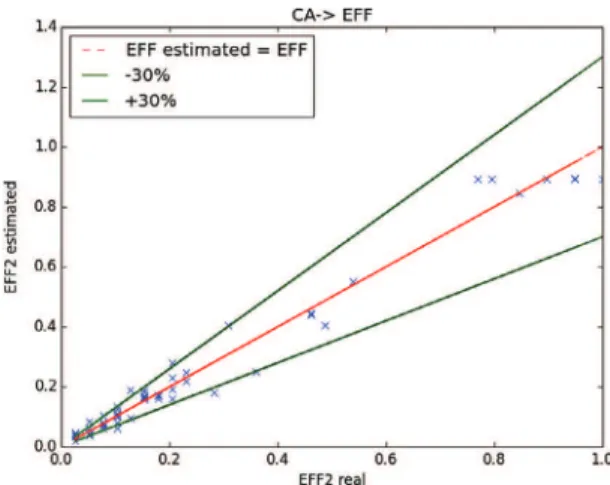
Next, an attempt is made to estimate manpower based on only sales data. The same methodology is used to identify the optimal network under a targeted error limit. The average error is fixed to 20%, and 52 tuples of values are used to train the ANN. A good result is obtained with an ANN with 4 layers
1, 16, 8, 1, as shown in Fig. 15. The results of the training step provide a satisfactory estimate of the manpower, with a majority of the estimated values under the 30% error target and an average error of 20%. After training, a set of 218 tuples of different values is tested to compare the ANN estimated values with the real values.
Fig. 13 – Output of the ANN looking for EFF with CA and EBE as inputs during the training step: scale 1->40.
Fig. 14 – Output of the ANN looking for EFF with CA and EBE inputs in the verification step: scale 1->40.
Fig. 15 – Output of the ANN looking for EFF with CA as input in the training step: scale 1->39.
As can be seen inFig. 16, the result is not satisfactory. There are some estimated values close to the real values, but only 117 points have error less than 30%, and 101 points are outside this acceptable boundary, resulting in accurate estimates for only 53% of the values. With respect to the linear regression, sales are definitively not representative of the number of jobs created and cannot be used to create a model for the estimation.
Fig. 16 – Output of the ANN looking for EFF with CA as input in the verification step: scale 1->40.
Fig. 17 – Output of the ANN looking for EFF2 with CA1, EFF1, CA2 as inputs in the training step: scale 1->172.
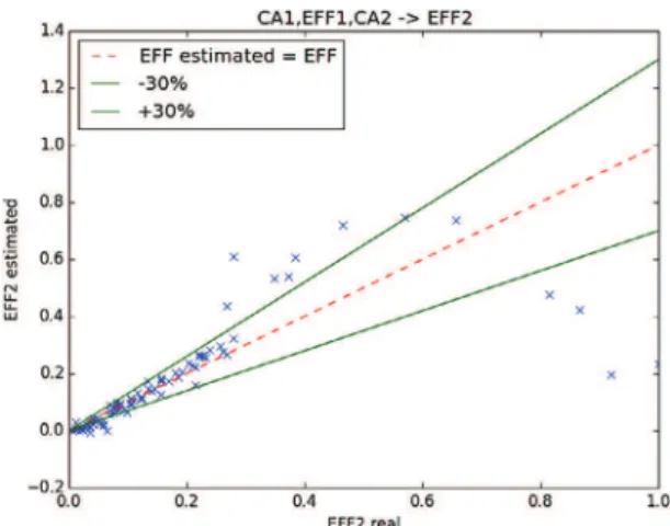
Another possibility is tested by estimating the variance of manpower for the same company at different times and with different sales volumes. However, only some data with one or two years of activity are available. Therefore, the result is limited. The same methodology is used. Tuples of values containing the sales and manpower for the first year and the sales for the second year are used. The expected result is the estimation of manpower for the second year. For improved efficiency, all the tuples where the manpower or sales do not change are erased, leaving 49 tuples with 44 under 0.4 (1 represents a manpower of 172) for the training step, and a good ANN with four layers is obtained 3, 12, 10, 1Fig. 17.
The result is better than that of the second test, as shown in Fig. 18. Here, 84 of the 91 values are under 0.4 on the ordinate axis, and in this area of the graph, the estimation is very close to the real values. There are 59 points with less than 30% error and 32 points with greater than 30% error for all sets of data, corresponding to 64% satisfactory results. However, under an EFF of 0.4, there are 58 points with error less than 30% and 32 points with error greater than 30%, giving an accuracy of 64.4%. Moreover, with an EFF between 0.1 and 0.4, the are 36 good points and only 5 bad points, for 84% good results. The authors believe that this result is a consequence of the fact that at a manpower near 0, the result quickly exceeds 30% error. Finally, the authors believe that the hypothesis based on the use of only sales from the same type of production is accurate in this case, even if the data account
Fig. 18 – Output of the ANN looking for EFF2 with CA1, EFF1, CA2 as inputs in the verification step: scale 1->172.
for only two or three years. However, the amount of data is not sufficient to confirm this conclusion. Therefore, it will be interesting to further explore this area if more significant data are found.
5.
Proposition
Relying on the previous results on manpower estimation using economic data, the main objective of this section is to propose a different formula to calculate direct jobs, indirect jobs, and induced jobs.
5.1. Direct jobs
As explained in the first section of this article, direct jobs are usually estimated based on the use of similar companies as references or on rules to determine the number of jobs for each workstation. In the previous section, the second and third formulae provide the best results. However, the results are not better in the third formula than in the second one, despite the introduction of a third coefficient. Therefore, the formula(21)can provide an initial estimate of the number of jobs created.
α ∗(V A − EBE) + β ≈ Manpower. (21)
5.2. Indirect jobs
The method found in the literature to estimate the number of indirect jobs generated by a company is the ratio between the sales (CA) of a company and total sales multiplied by manpower. However, as previously explained, manpower is not linearly related to sales or investment (according to the literature and experiments performed in this article). Therefore, a possible approach is based on two estimates of the manpower of the company: one without the new activity and the other with it. The difference between the two values enables estimation of the impact of this activity on the number of jobs. This approach has the advantage of considering the possible nonlinearity in manpower, therefore reducing the error margin in the estimate. Two methods from a previous study are proposed for this estimation: the first one is to estimate the direct jobs of a subcontractor based on the relation between VA, EBE and manpower, that is to
say, estimating the direct jobs for a subcontractor considering the modification of the activity; the second is based on the variation of sales using a trained ANN, as in the last study. This last method appears to have an acceptable error margin.
5.3. Induced jobs
The number of induced jobs is more difficult to evaluate. A statistical evaluation is often used in the literature. Due to the limited availability of input data mentioned in Section2.3, the authors propose a simplification of Eq. (3). Instead of using the local ratios corresponding to the portion of workers supported by household consumption (PWLP in Eq.(22)), the authors propose the use of the portion of the gross domestic product (GDP) supported by household consumption in the different sectors of economic activity. The main advantage of this formula is that the GDP is easier to obtain than the part of local workers supported by the local population, and it can be specified by activity sector. Therefore, the proposed formula is:
InducedJobssector=JIA ∗ GDPsector∗
(DJ + IJ) ∗ SF P . (22) • The number of direct jobs: DJ
• The number of indirect jobs: IJ
• The average household size in the location of the activity: SF
• The size of the population: P
• The portion of GDP, by sector, supported by household consumption: GDPsector
• Number of jobs in the study area: JIA.
The portion of GDP due to household consumption is not the same as the household consumption estimated as a percentage of PIB, as proposed by the World Bank ( world-bank.org/, 2016), but it corresponds to the portion of GDP impacted by household consumption. For example, in France in 2011, household consumption was 55% of GDP (≈ 1110.1 bil-lion euros (economie.gouv.fr lafinancepourtous.com, 2013)) and it impacted 30% of the national GDP (economie.gouv.fr lafinancepourtous.com, 2013).
6.
Case study
6.1. Biomass supply chainThe biobased economy is a promising way to contribute significantly to long-term sustainable development. The pro-duction of biobased derivatives converts biomass into a wide spectrum of biomolecules, biochemicals, biomaterials or bio-fuels. Furthermore, these biorefineries are expected to meet all the challenges of sustainability, which imply a trade-off between economic viability, environmental impact and social impact. The case study specifically addresses the optimal design of the bioethanol supply chain in France as it can be used as gasoline alternative because of its compatibility with automobile engines. This work focuses on multi-objective optimization by considering minimization of the total costs (investment and operating costs), minimization of the Eco-Cost for the environmental criteria and the total number of jobs created for the social dimension. For the latter, the num-ber of direct jobs is calculated with the second formulation with the coefficient values corresponding to the chemical sector (Table 5). The number of direct (or indirect) jobs is estimated with Eq.(2)(or Eq.(22)) and the method described
in Section5.2(or5.3). The main objective of this study is to find a solution that reaches a compromise between the three previous criteria to help the decision maker to select locations to establish one or more refineries.
After all the possible alternatives are described, the op-timization problem is formulated as a mixed integer linear program that accounts for biomass seasonality, geographical availability, biomass degradation, process conversion tech-nology and final product demand. After a sales forecast, the annual production is estimated to be 400,000 ton/year. The output results of the model give the optimal network design, facility locations and size, process selection and inventory location, size, and policy. The multi-objective optimization of the biomass supply chain relies on a multi-scale framework to provide a holistic view and to integrate its different compo-nents. The model description and the specific multi-objective optimization methods are detailed in Miret et al.(2016) (not the purpose here).
6.2. Multi-objective optimization
In this section, the results obtained in the previous work are summarized. First, single optimization problems are con-sidered. InTable 8, each row represents a mono-objective optimization with the objective function that is being mini-mized or maximini-mized, and at the optimum point, the value of the decision variables are used to evaluate the other criteria. The results for each are presented in columns (the values on the diagonal are the optimum values for each mono-objective optimization).
The main conclusions are that the criteria are antagonistic and that the range of each criterion is large. More precisely, due to the range of variation, the economic dimension is antagonistic with the environmental dimension and very antagonist with the social dimension. Furthermore, to re-flect the decision maker’s choice, we can attach a weight to each criterion. If balanced weights are applied to the model, acceptable environmental criteria and employment are obtained, but the economic costs are high. On the other hand, if a greater weight is applied to the economic criteria, the Eco-Cost doubles, and employment is halved. Different coefficient weights are tested to explore the solution space. InTable 9, we summarize the three points obtained despite many coefficients, highlighting the difficulty in finding a balance between the three criteria. The first row of the table gives the weights for each criterion for the three different results (columns 2, 3 and 4). In the following rows, the three criteria are reported along with the most important decision variables, in particular, the location and the capacity for both the refineries and the storage sites. For each criteria, the relative difference with respect to the best solution reached during mono-objective optimization is given in parentheses. The values of these optimal solutions are also reported in the last column, which represent a utopian point that would be the optimal solution if it could be reached. The first comment onTable 9 concerns the capacity of the refineries. For the first two solutions (columns 2 and 3), the production capacity is higher than the planned capacity, whereas for the last solution (column 4), the refinery is working at full capacity. To explain this result, let us focus on solution 4, where the economic criterion has a higher relative weight. One biorefin-ery working at full capacity is economically more interesting than building two or more biorefineries, but it sharply reduces
the number of jobs created (economy of scale). As the eco-nomic and social criteria are very antagonistic, the difference between weights leads to a more economical solution. As a result, both the economy of scale and the reduction of operating costs (decrease in wage costs) contribute to the reduction in direct jobs and, as a consequence, to a de-crease in the number of indirect and induced jobs (as the latter is proportional to the former two, Eq.(22)). Inversely, when the relative weight of the social criterion increases, the number and capacity of biorefineries increase to improve the total number of accrued jobs. Furthermore, it is also important to note that the biorefineries are located in more rural cities, leading to an increase in induced jobs. Storages sites are reduced to become more realistic and to reach a compromise between the antagonistic economic and social dimensions. The greater the attenuation of the relative differ-ence between the weight of economic and societal criteria is, the more the previous findings are highlighted (comparison between solutions 1 and 2): production capacity overshot, biorefineries located in more rural cities, and storage capacity minimized.
It is also important to note that the plant location is also driven by cost. For solution 3, if we prohibit the location in crowded cities (e.g., Bordeaux), the simulation results al-ways give one refinery with a production capacity of 400,000 ton/years located in a smaller proximate city (e.g., Pau). The main differences between the two previous solutions are:
• While the numbers of direct and indirect jobs are the same, Pau is a more rural city; as a consequence, the number of induced jobs is slightly increased.
• The geographical position of Pau is less central; as a consequence, the supply chain costs are increased, which is why Bordeaux is selected in the simulation without prohibition.
In conclusion, for solution 3, the social criterion does not influence biorefinery production capacity and location; its im-pact is only visible on storage. While this solution satisfies the mathematical constraints of the problem, it is not relevant because the number and capacity of storage sites increase sharply relative to solutions 1 and 2. Indeed, the number and capacity of storage sites have limited influence on the economic criterion but greater influence on job creation. As a consequence, they increase or become excessive to satisfy the social criteria. Moreover, these storage sites are located in more rural cities to increase the induced jobs. When the social criterion becomes more important in decision making, the number and capacity of biorefineries increase to improve the total number of accrued jobs. Indeed, due to capacity growth, the number of direct and indirect jobs increase and, as a consequence, the number of induced jobs also increases. Furthermore, it is important to note that biorefineries are located in more rural cities, leading to an increase in in-duced jobs. Concerning storage sites, they are rein-duced to become more realistic to reach a compromise between the antagonistic economic and social dimensions. The greater the attenuation of the relative difference between the weights of the economic and societal criteria is, the more the previous findings are highlighted. This analysis is obtained from the comparison between solutions 1 and 2. In solution 1, the production capacity is overshot to satisfy the social criteria. In the same way, biorefineries are located in more rural cities. By contrast, the storage capacity reaches its minimum and optimal value.