1 Bivariate index-flood model for a northern case study
1
M.-A. Ben Aissia* 1 2 F. Chebana 1 3 T. B. M. J. Ouarda 1,2 4 P. Bruneau 3 5 M. Barbet 3 6 1
Statistics in Hydrology Working Group. Canada Research Chair on the Estimation of 7
Hydrological Variables, INRS-ETE, 8
490, de la Couronne, Quebec, (Quebec) Canada, G1K 9A9. 9
2
Institute Center for Water and Environment (iWATER) 10
Masdar Institute of Science and Technology, 11
PO Box 54224, Abu Dhabi, UAE. 12
3
Hydro-Québec Équipement 13
855, Ste-Catherine East, 19th Floor, Montreal (Quebec) Canada, H2L 4P5. 14
* Corresponding author: mohamed.ben.aissia@ete.inrs.ca
15 16 17 October 2013 18 19
2 20
Abstract
21
Floods, as extreme hydrological phenomena, can be described by more than one 22
correlated characteristic such as peak, volume and duration. These characteristics should 23
be jointly considered since they are generally not independent. For an ungauged site, 24
univariate regional flood frequency analysis (FA) provides a limited assessment of flood 25
events. A recent study proposed a procedure for regional FA in a multivariate framework. 26
This procedure represents a multivariate version of the index-flood model and is based on 27
copulas and multivariate quantiles. The performance of the proposed procedure was 28
evaluated by simulation. However, the model was not tested on a real-world case study 29
data. In the present paper, practical aspects are investigated jointly for flood peak (Q) and 30
volume (V) of a data set from the Côte-Nord region in the province of Quebec, Canada. 31
The application of the proposed procedure requires the identification of the appropriate 32
marginal distribution, the estimation of the index flood and the selection of an appropriate 33
copula. The results of the case study show a good performance of the regional bivariate 34
FA procedure. This performance depends strongly on the performance of the two 35
univariate models and more specifically the univarite model of Q. Results show also the 36
impact of the homogeneity of the region on the performance of the univariate and 37
bivariate models. 38
39 40
3
1. Introduction and literature review
41
A flood can be described as a multivariate event whose main characteristics are peak, 42
volume and duration. Thus, the severity of a flood depends on these characteristics, 43
which are mutually correlated (Ashkar 1980, Yue et al. 1999, Ouarda et al. 2000, Yue 44
2001, Shiau 2003, De Michele et al. 2005, Zhang and Singh 2006, Chebana and Ouarda 45
2009, Chebana and Ouarda 2011). These studies show that these variables have to be 46
jointly considered. 47
The use of joint probabilistic behaviour of correlated variables is necessary to understand 48
the probabilistic characteristic of such events. Yue et al. (1999) used the bivariate 49
Gumbel mixed model with standard Gumbel marginal distributions to represent the joint 50
probability distribution of flood peak and volume, and flood volume and duration. 51
Ouarda et al (2000) were first to study the joint regional behaviour of flood peaks and 52
volume. To model flood peak and volume, Yue (2001) and Shiau (2003) used the 53
Gumbel logistic model with standard Gumbel marginal distributions. Recently, copulas 54
have been shown to represent a useful statistical tool to model the dependence between 55
variables. To model flood peak and volume with Gumbel and Gamma marginal 56
distribution respectively Zhang and Singh (2006) used the copula method, bivariate 57
distributions of flood peak and volume, and flood volume and duration in frequency 58
analysis (FA). Using the Gumbel–Hougaard copula, Zhang and Singh (2007) derived 59
trivariate distributions of flood peak, volume and duration in FA. 60
Generally, the record length of the available streamflow data at sites is much shorter than 61
the return period of interest and in some cases, there may not be any streamflow record at 62
4 these sites. Consequently, local frequency estimation is difficult and/or not reliable. 63
Regional FA is hence commonly used to overcome this lack of data. It is based on the 64
transfer of available data from other stations within the same hydrologic region into a site 65
where little or no data are available. The regional FA procedure was investigated with 66
different approaches by several authors including Stedinger and Tasker (1986), Rocky 67
Durrans and Tomic (1996), Nguyen and Pandey (1996), Hosking and Wallis (1997), Alila 68
(1999, 2000) and Ouarda et al. (2001). GREHYS (1996a, 1996b) presented an 69
intercomparison of various regional FA procedures. 70
In the literature, flood FA can be classified into four classes according to the 71
univariate/multivariate and local/regional aspects. The local-univariate and regional-72
univariate classes were widely studied in the literature (Singh 1987, Wiltshire 1987, Burn 73
1990, Hosking and Wallis 1993, Hosking and Wallis 1997, Alila 1999, Ouarda et al. 74
2006, Nezhad et al. 2010). Recently, researchers have been increasingly interested in the 75
multivariate case and many studies treated the problem of local-multivariate flood FA 76
(Yue et al. 1999, Yue 2001, Shiau 2003, De Michele et al. 2005, Grimaldi and Serinaldi 77
2006, Zhang and Singh 2006, Chebana and Ouarda 2011). However, multivariate 78
regional FA has received much less attention (Ouarda et al. 2000, Chebana and Ouarda 79
2007, Chebana and Ouarda 2009, Chebana et al. 2009). 80
The two main steps of the regional FA are the delineation of hydrological homogeneous 81
regions and regional estimation (GREHYS 1996a). In the multivariate case, the 82
delineation of hydrological homogeneous regions was treated by Chebana and Ouarda 83
(2007). They proposed discordancy and homogeneity tests that are based on multivariate 84
L-moments and copulas. Chebana et al. (2009) studied the practical aspects of these tests. 85
5 In univariate-regional FA, different methods were proposed to estimate extreme quantiles 86
such as regressive models and index-flood models (e.g. GREHYS 1996a, 1996b). 87
Chebana and Ouarda (2009) proposed a procedure for regional FA in a multivariate 88
framework. The proposed procedure represents a multivariate version of the index-flood 89
model. In this method, it is assumed that the distribution of flood characteristics (flood, 90
peak or volume) at different sites within a given flood region is the same except for a 91
scale parameter. Chebana and Ouarda (2009) adopted the multivariate quantile as the 92
curve formed by the combination of variables corresponding to the same risk (Chebana 93
and Ouarda 2011). In order to model the dependence between variables describing the 94
event they employed the copula. In the present paper, practical aspects of the proposed 95
procedure by Chebana and Ouarda (2009) are studied. Real data sets from sites in the 96
Côte Nord region in the northern part of the province of Quebec, Canada are used. Flood 97
peak and volume are the two variables studied jointly in the present study. 98
The next section presents the theoretical background, including the bivariate modelling, 99
univariate index-flood model and multivariate quantiles. The “Multivariate Index-flood 100
Model” section details the methodology of the adopted procedure with an emphasis on 101
practical aspects. The case study section presents the study procedure as well as the 102
obtained results. Concluding remarks are presented in the last section. 103
2. Background
104
In this section, the background elements to apply the index-flood model in the 105
multivariate regional FA procedure are presented. Bivariate modelling including copulas 106
6 and marginal distributions, univariate index-flood model and multivariate quantiles are 107
briefly described. 108
II.2.1. Bivariate flood modelling and copulas
109
In bivariate modelling, a joint bivariate distribution for the underlying variables has to be 110
obtained. According to Sklar’s theorem (1959), the bivariate distribution is composed of 111
a copula and two margins which are not necessarily similar. 112
In the remainder of the paper, we denote FX and FY respectively the marginal distribution
113
functions of given random variables X and Y, and FXY the joint distribution function of the
114
vector (X,Y). 115
a) Copula
116
Due to its ability to overcome the limitation of classical joint distributions, copulas have 117
received increasing attention in various fields of science (see e.g. Nelsen 2006). Copulas 118
are used to describe and model the dependence structure between the two random 119
variables. A copula is an independent function of marginal distributions. For more details 120
on copula functions, see for instance Nelsen (2006), Chebana and Ouarda (2007) and 121
Salvadori et al. (2007). According to Sklar’s (1959) theorem, we can construct the 122
bivariate distribution FXY with margins FX and FY by:
123
,
,
XY X Y
F x y C F x F y for all real x and y (1)
When FX and FY are continuous, the copula C is unique.
124
Different classes of copulas are studied in the literature such as the Archimedean, 125
Elliptical, Extreme Value (EV), Plackette and Farlie-Gumbel-Morgenstern (FGM) 126
7 copulas (see e.g. Nelsen 2006, Salvadori et al. 2007). The use of a copula requires the 127
estimation of its parameters as well as goodness-of-fit procedures. In addition, since in 128
hydrology we are particularly interested by the risk, the tail dependence of copulas is also 129
a factor to take into account. 130
Copula parameter estimation: Assuming the unknown copula C belongs to a parametric
131
family C0
Cθ:θRq
;q2. The estimation of the parameter vector θ is the first step to132
deal with. In the case of one-parameter bivariate copula, a popular approach consists of 133
using the method of moment-type based on the inversion of Spearman’s ρ and Kendall’s 134
τ. Demarta and McNeil (2005) have shown that such approach may lead to 135
inconsistencies. The maximum pseudo-likelihood (MPL) approach is shown to be 136
superior to the other ones (Besag 1975, Genest et al. 1995, Shih and Louis 1995, Kim et 137
al. 2007) in which the observed data are transformed via the empirical marginal 138
distributions to obtain pseudo-observations on which the maximum-likelihood approach 139
is based to estimate the associated copula parameters (Genest et al. 1995). The advantage 140
of this approach is that it can provide greater flexibility than the likelihood approach in 141
the representation of real data. It consists in maximizing the log pseudo-likelihood: 142
1 ˆ log log n i i L c U
(2)where
c
denotes the density of a copula CθC0, and Uˆk
UˆkX,UˆkY
are the pseudo-143
observation obtained from
XkYk
given by:144 kl ˆ U , 1,..., ; or 1 kl R k n l X Y n (3)
with RkX being the rank of Xk among X1,…,Xn and RlY being the rank of Yl among Y1,…,Yn.
8
Goodness-of-fit test: The most important step in copula modelling is the copula selection
146
by the goodness-of-fit test. Formally, one wants to test the hypotheses: 147
0: 0 against 1: 0
H CC H CC (4)
Due to the novelty of copula modelling in flood FA, there is no common goodness-of-fit 148
test for copulas. One of the most commonly used goodness-of-fit tests and valid only for 149
Archimedean copulas is the graphic test proposed by Genest and Rivest (1993) based on 150
the K function given by 151
0 1 u u u u u K (5)where is the generator function of the Archimedean copula. The K function can be
152 estimated by 153
, i 1,..,N 1 1 1 where 1 1 ˆ 2 2 1 1 , 1
i t i t i u u u u i N i u w N w N u K (6)for a given bivariate sample
u u
u u
u1N u2N
2 2 2 1 1 2 11, , , , . . . , , . Genest and Revest (1993) have
154
shown that Kˆ is a consistent estimator of K under weak regularity conditions. Note that
155
Archimedean copulas are widely employed in hydrology and particularly to model flood 156
dependence. 157
Recently, a relatively large number of goodness-of-fit tests were proposed (see e.g. 158
Charpentier 2007, Genest et al. 2009, for extensive reviews). Genest et al. (2009) carried 159
out a power study to evaluate the effectiveness of various goodness-of-fit tests and 160
recommended a test based on a parametric bootstrapping procedure which makes use of 161
the Cramer-von Mises statistic Sn (Sn goodness-of-fit test) :
9
nC u v C u v dC u v Sn n , n , n , 2 (7)where Cn is the empirical copula calculated using n observation data. and Cθn is an
163
estimation of C obtained assuming
C
C
0. The estimation Cθn is based on the estimator164
θn of θ such as the maximum pseudo-likelihood estimator given in (2).
165
b) AIC for copula
166
In some cases, results of the goodness-of-fit testing show that more than one copula 167
provide a good fit to the data set. To select the most adequate copula, we use the AIC 168
(Akaike's information criterion) proposed by Kim et al. (2008) in the context of copulas: 169
ˆ 2 log( ( ; , )) 2 ; ˆ ˆ ( ; , ) log X( ), Y( ), AIC L X Y r L X Y c F X F Y
(8)where is the estimation of the copula parameter vector θ, r is the dimension of θ and c ˆ
170
is the copula density. 171
The copula which has the lowest AIC value is the most adequate copula for the data set. 172
c) Marginal distributions
173
To selection of the most appropriate marginal distribution (for X and for Y). The choice of 174
the appropriate distribution is based on the Chi-square goodness-of-fit test, graphics and 175
selection criteria (AIC see e.g. Akaike (1973) and BIC see e.g. Schwarz (1978)). For 176
parameter estimation, a number of methods are available in the literature to estimate 177
marginal distribution parameters; such as, the method of moments, the maximum 178
likelihood method and the L-moments method. 179
10
II.2.2. Univariate Index-flood model
180
Introduced by Dalrymple (1960), the index-flood model was used initially for regional 181
flood prediction. It is also used to model other hydrological variables including storms 182
and droughts (e.g. Pilon 1990, Hosking and Wallis 1997, Hamza et al. 2001, Grimaldi 183
and Serinaldi 2006). This model is based on the assumption of the homogeneity of the 184
considered region and all the sites in the region have the same frequency distribution 185
function apart from a scale parameter specific to each site. Let Ns be the number of sites
186
in the region. The model gives the quantile Qi(p) corresponding to the non-exceedance
187
probability p at site i as: 188
( ) , 1 and 0 1
i i s
Q p q p i ,....,N p (9)
where μi corresponds to the index flood and q is the regional growth curve.
189
The index flood parameter μi can be estimated using a number of approaches (Hosking
190
and Wallis 1997). For instance, Brath et al. (2001) used three models of estimating the 191
index flood parameter. These models are multi-regression model, rational model and 192
geomorphoclimatic model. They show that best results are given by considering the 193
multi-regression model of the form: 194 3 1 2 0 1 2 3 ˆ a a a... an i a A A A Anp (10)
in which ai are coefficients to be estimated, and Ai,…, Anp represent an appropriate set of
195
morphological and climatic characteristics of the basin such as watershed area and slope 196
of the main channel. 197
11
II.2.3. Multivariate quantiles
198
Unlike to the well-known univariate quantile, the multivariate quantile has received less 199
attention in hydrology. Despite that, a few studies proposed multivariate quantile 200
versions. For details, the reader is referred to Chebana and Ouarda (2011). The pth 201
bivariate quantile curve for the direction ε is defined as: 202
2
, , : ,
XY
q p x y R F x y p (11)
with pI is the risk and F(x,y) is the bivariate cumulative distribution function given 203
by: 204
,
Pr
,
F x y X x Yy (12)
which represents the probability of the simultaneous non-exceedance event. Other events 205
can also be considered (see Chebana and Ouarda 2011 for more details). 206
The bivariate quantile in (10) is a curve corresponding to an infinity of combinations (x,y) 207
that satisfiesF x y
,
p. For the event
X x Y, y
, using (2) and (10), the quantile 208curve can be expressed as follows: 209
2 1 1 , such that , ; , 0,1 : , X XY Y x y R x F u q p y F v u v C u v p (13)The index-flood model used in this paper is based on (12). The resolution of (12), using 210
copula and margin distribution, gives an infinity of combinations (x,y). These 211
combinations constitute the corresponding quantile curve. The main properties of the 212
index-flood model are (see Chebana and Ouarda 2011 for more details): 213
1. The marginal quantiles are special cases of the bivariate quantile curve. Indeed, they 214
correspond to the extreme scenarios of the proper part related to the event; 215
12 2. The bivariate quantile curve is composed of two parts: naïve part and proper part. 216
The proper part is the central part whereas the naïve part is composed of two 217
segments starting at the end of each extremity of the proper part; 218
3. When the risk p increases, the proper part of the bivariate quantile becomes shorter. 219
3. Multivariate index-flood model in practice
220
The following procedure is proposed by Chebana and Ouarda (2009) and represents a 221
complete multivariate version of regional FA. Since Chebana and Ouarda (2009) 222
represent a theoretical study, we propose in the present paper a methodology of 223
application of this procedure on a real world case study. The multivariate index-flood 224
model regional estimation requires the delineation of a homogeneous region. 225
The step of delineation of a homogeneous region is treated by Chebana and Ouarda 226
(2007) in the multivariate case. Based on multivariate L-moments, they proposed 227
statistical tests of multivariate discordancy D and homogeneity H. The practical aspects 228
of these tests are studied in Chebana et al. (2009). 229
The estimation procedure of the extreme event by the multivariate index-flood model is 230
developed by Chebana and Ouarda (2009). It consists in extending the index-flood model 231
to a multivariate framework using copula and multivariate quantiles. In this step, the 232
homogeneity of the region is assumed. Indeed, non-homogeneous sites must be removed 233
in the first step. 234
13 Let N' be the number of sites in the homogeneous region with record length ni at site i,
235
1,..., '.
i N The goal is to estimate, at the target site l, the bivariate and marginal 236
quantiles corresponding to a risk p. 237
Let
x yij, ij
for i1,...,N';j1,..., ,ni be the data where x and y represent the observations of 238the considered variables. Let qp be the regional growth curve which represents a quantile
239
curve common to the whole region. 240
The complete procedure of determination of the bivariate quantile curve for an ungauged 241
site is described as follows: 242
1. Identify the homogeneous region to be used in the estimation as follows: to 243
identify and remove discordant sites, apply the multivariate discordancy test D 244
and check the homogeneity of the remaining sites by the homogeneous test H. In 245
practice, it's very difficult to find an exactly homogeneous region. According to 246
Hosking and Wallis (1997), approximate homogeneity is sufficient to apply a 247
regional FA, in the multivariate framework, this procedure was developed by 248
Chebana and Ouarda (2007) and results will be used in this paper. 249
2. Assess the location parameters μiX and μiY i=1,…,N’ and standardize the sample
250 (xij,yij), j=1,…,ni to be: 251 , ij ij ij ij iX iY x y x y (14)
3. Select the bivariate distribution which is composed of a copula and two margins. 252
In this step, our goal is to identify adequate marginal distributions and copula for 253
the whole region to fit the standardized data
xij',yij'
. This step is described as 254follows: 255
14 a) Collect the data from the homogeneous region to get a sample xk'',yk'' 256 ' 1 1,..., ; N i i k n n n
. This sample will be used to select the marginal 257distributions and copula. 258
b) Identify the adequate marginal distributions (for X and for Y) using the 259
AIC, BIC and graphical criteria. 260
c) Select the adequate copula using the graphic test proposed by Genest and 261
Rivest (1993) and the AIC criterion. 262
4. For each site i, i=1,…,N’, estimate the parameters of marginal distributions and 263
copula family selected in step 3. For the copula family, the MPL method is used 264
to estimate the copula parameter. However, for marginal distributions, the 265
estimation method depends on the marginal distribution. Let i k
ˆ be the estimator
266
of the kth parameter from the standardized data of the ith site k=1,…, s; s is the 267
number of parameters to be estimated, i1,...,N'. Obtain the weighted regional 268 parameter estimators: 269 ' 1 ' 1 ˆ ˆ , 1,..., N i i k r i k N i i n k s n
(15)5. For a given value of risk p, estimate different combinations of the estimated 270
growth curve qˆx,y
p from (12) using the fitted copula with the corresponding271
weighted regional parameter R k
ˆ with k=1,…, s. 272
6. Estimate the index flood parameter by a multivariate multiple regression model 273
15 where μ is the index flood vector, A is the matrix of watershed physiographic 274
characteristics, E is the matrix of coefficients to estimate and ε is the error. The 275
estimation of index flood can be separated into two steps: 276
a) Choice of physiographic characteristics: the aim of this step is to select, from 277
a list of physiographic characteristics, the optimal set of physiographic 278
characteristics to be considered in the model. Here, the order of 279
characteristics in the selected set is important. The method of multivariate 280
stepwise regression based on the Wilks statistics was used (see e.g. Rencher 281
2003). 282
b) Estimation of the coefficients E: the method of maximum likelihood is used 283
(Meng and Rubin 1993). 284
7. Multiply each growth curve combination with the vector of index flood of the 285 target l: μlX and μlY 286
ˆr
lX ˆ
, 0 p 1 xy xy l lY μ Q p q p μ (17)Hence, the obtained result in (16) is an estimation of the bivariate regional quantile 287
associated to the risk p. 288
To evaluate the performance of the regional FA models, Hosking and Wallis (1997) 289
suggested an assessment procedure that involves generation of regional average L-290
moments through a Monte Carlo simulation. This procedure is based on the Jackknife 291
resampling procedure (e.g. Chernick 2012). It consists in considering each site as an 292
ungauged one by removing it temporarily from the region and estimating the bivariate 293
and univariate regional quantiles for various nonexceedance probabilities p in the 294
simulations. This is similar, for instance, to Ouarda et al (2001) in the regional frequency 295
16 analysis context. At the mth repetition, the regional growth curves and the site i quantiles 296
are computed. 297
As indicated in Chebana and Ouarda (2009), the performance of the corresponding 298
bivariate regional FA model cannot be evaluated on the basis of the usual performance 299
evaluation criteria. The evaluation is based on the deviation between the regional and 300
local quantile estimated curves. The quantile curve is denoted by (x, Gp(x)). The relative 301
error between the regional and local quantile curves is given by: 302
r l p p p l p G x G x R x G x (18)where exponents r and l referring respectively to regional and local quantile curves. 303
This relative difference represents vertical point-wise distances between the two quantile 304
curves. In order to evaluate the estimation error for a site I, Chebana and Ouarda (2009) 305
proposed the bias and root-mean-square error respectively given by 306
2 1 1 100 1 * and 100 M M i m m m m m B p REI p R p REI p M M
(19)where M is the number of simulations, REI* and REI are the two relative integrated error 307
of the simulation m defined respectively by 308
1
* , 0 1 p p p QC REI p R x dx p L
(20)
1
, 0 1 p p p QC REI p R x dx p L
(21)with Lp is the length of the proper part of the true quantile curve QCp for the risk p. 309
To summarize these criteria over the sites of the region, it is possible to average them to 310
obtain the regional bias, the absolute regional bias and the regional quadratic error given 311
respectively by 312
17
1 1 1 1 1 1 N i i N i i N i i RB p B N ARB p B N RRMSE p R N
(22)4. Case study
313The application of the index-flood model in a multivariate regional FA framework 314
concerns a regional data set of interest for the Hydro-Québec Company. The two main 315
flood characteristics, that is, volume V and peak Q are jointly considered. These flood 316
features are random by definition since they are based on the flood starting and ending 317
dates. The latter are obtained using an automatic method which consists in the analysis of 318
cumulative annual hydrographs by adjusting the slopes with a linear approximation (e.g. 319
Ben Aissia et al. 2012). The employed data is used in Chebana et al. (2009). They are 320
from sites in the Côte Nord region in the northern part of the province of Quebec, 321
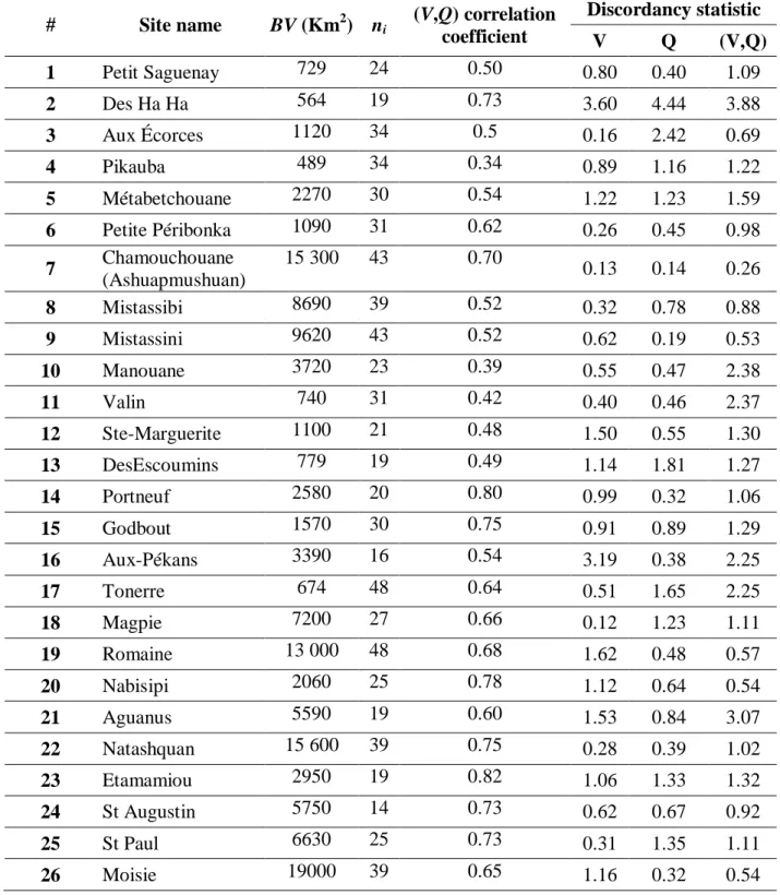
Canada. The number of sites in the region is N=26 stations with record lengths ni between
322
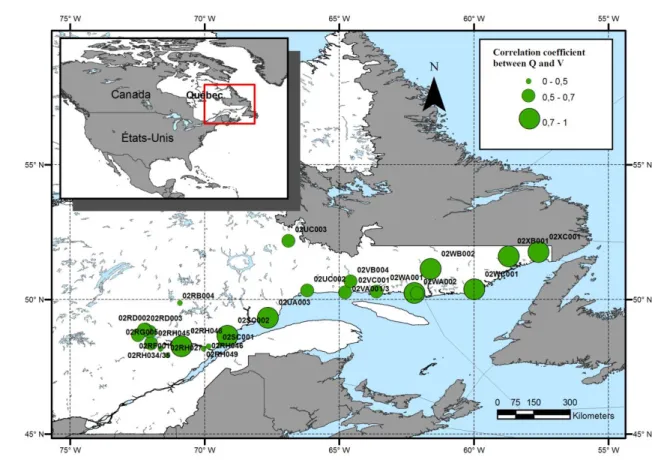
14 and 48 years. More information about the data is given in Table 1. Figure 1 presents 323
the geographical location and the correlation coefficient between Q and V for the 324
underlying sites. 325
II.4.1. Study procedure:
326
The procedure of the study is composed of the following eight steps: 327
1. Delineate the homogeneous region; 328
2. Assess the location parameters μiV and μiQ for i = 1,…, N’ given by (13);
18 3. Select a family of regional multivariate distributions to fit the standardized data of 330
the whole region; 331
4. For each site in the homogeneous region, estimate the parameters of the marginal 332
distributions and copula family. Estimate the regional parameter estimator ˆ R k
by
333
(14); 334
5. Estimate different combinations of the estimated growth curve qˆv q, p from (12); 335
6. Estimate the index flood by a multiregression model (15); 336
7. Using (16), estimate the bivariate regional quantiles associated to the risk p; 337
8. For each flood characteristic, estimate the univariate regional growth curve and 338
using (8) estimate the univariate regional quantile; 339
9. Evaluate the performance of the regional models (univariate and bivariate) by 340
Monte Carlo simulation. 341
II.4.2. Result and discussion
342
In this section, results of the application of the adopted procedure are presented. First, 343
results of the multivariate homogeneity study are briefly presented followed by the results 344
of the index-flood regional estimation. 345
Discordancy and homogeneity
346
The employed data is the same used in Chebana et al. (2009) and the discordancy and 347
homogeneity results are presented in that reference and in Table 1.The sites that may be 348
discordant have a large discordancy value. Results show that: 349
- Sites 2 and 16 are discordant for V; 350
19 - Site 2 or sites 2 and 3 are discordant for Q;
351
- Sites 2 and 21 are discordant for (V,Q). 352
The two sites 2 and 21 are eliminated to allow application of the respective homogeneity 353
test. Table 2 presents the homogeneity test values for the region for V, Q and (V,Q) after 354
removing the two discordant sites (2 and 21). From Table 2, according to the statistic H, 355
we conclude that the region is homogeneous for V, heterogeneous for Q and could be 356
homogeneous for (V,Q). 357
Identification of marginal distributions
358
In regional FA, a single frequency distribution is fitted from the whole standardized data. 359
In general, it will be difficult to get a homogeneous region, consequently there will be no 360
single “true” marginal distribution that applies to each site (Hosking and Wallis 1997). 361
Therefore, the aim is to find a marginal distribution that will yield accurate quantile 362
estimates for each site. The scale factor of this marginal distribution changes from one 363
site to another. 364
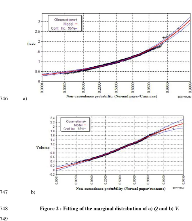
Figure 2 shows that the adequate marginal distributions are Gumbel for Q and GEV for 365
V. Results for the appropriate marginal distributions are in agreement with those of
366
similar studies e.g. Cunnane and Nash (1971) and De Michele and Salvadori (2002). 367
Identification of copula
368
Table 1 indicates that the dependence between V and Q varies from 0.34 to 0.82 while 369
Figure 1 shows that the dependence variability is scattered over the entire study area. The 370
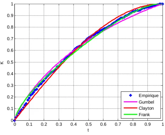
graphic test based on the K function (5) with the estimate (6) is applied for the three 371
20 Archimedean copulas: Gumbel, Frank and Clayton. This test leads to fitting the Frank 372
copula to the bivariate data for the studied region. The illustration of this fitting is 373
presented in Figure 3. 374
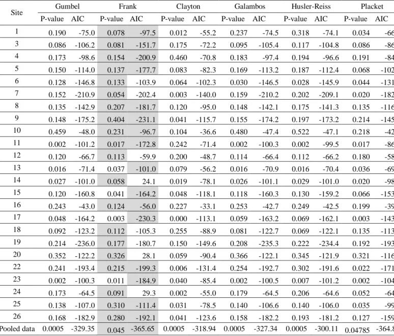
The AIC and p-value of the Sn goodness-of-fit test described earlier and proposed by
375
Kojadinovic and Yan (2009) are also calculated for the commonly considered copulas in 376
hydrology. However, direct results show that none of the commonly used copulas in 377
hydrology can be accepted. Even though, the graphic test based on the K function 378
indicates excellent fitting with Frank copula, the Sn goodness-of-fit test rejects this
379
copula, as well as the other ones being considered. First, the reason may be that 380
numerical tests tend to be narrowly focused on a particular aspect of the relationship 381
between the empirical copula and the theoretical copula and often try to compress that 382
information into a single descriptive number or test result (see e.g. NIST 2013). Second, 383
the test is widely and successfully applied to at-site hydrological studies which is not the 384
case for regional studies where the total sample size is very large (here n=714). The 385
performance of Sn goodness-of-fit test could be affected when the sample size is large as
386
indicated in Genest et al. (2009). In addition, in terms of application, Vandenberghe et al. 387
(2010) indicated limitation of this test for long sample size like in rainfall. Therefore, to 388
overcome this situation, this test is applied to the data series of each site separately. This 389
is justified since basically regional FA assumes the same distribution in each site apart 390
from a scale factor (see e.g. Hosking and Wallis 1997, Ouarda et al. 2008). However, 391
according to Hosking and Wallis (1997), it is difficult in practice to have a single 392
distribution which provides a good fit for each site. The goal is hence to find a 393
distribution that will yield accurate quantile estimates for all sites. For the present case-394
21 study, results (Table 3) show that Frank is the most accepted copula in the study sites 395
(accepted by the Sn goodness-of-fit test for 20 sites and sorted best by AIC for 17 sites
396
among 24 sites). Frank copula has already been shown to be adequate to model the 397
dependence between flood V and Q in a number of hydrological studies (see e.g. 398
Grimaldi and Serinaldi 2006). Finally, based on the above arguments (at-site Goodness-399
of-fit selection, regional graphic test based on the K function, regional and at-site AIC, 400
hydrological literature), the Frank copula is selected for the present case-study. 401
Therefore, the appropriate copula is Frank defined by: 402
,
1 ln 1
1
1
; 0 ; 0 , 1 ln 1 u v C u v u v (23)where γ is the parameter to be estimated. The choice of the adequate copula is in 403
agreement with those of similar studies e.g Lee et al. (2012). 404
Estimation of parameters associated to margins and copula
405
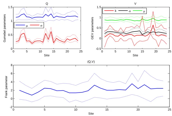
Parameters of marginal distributions and copula for each site and their corresponding 406
confidence intervals are presented in Figure 4 while Table 4 showing the regional 407
parameters of the marginal distributions and copula determined by (14). The MPL is 408
employed for the copula parameter. For the Gumbel distribution, μ and σ represent, 409
respectively, the location and scale parameters whereas for the GEV distribution, μ, σ and 410
k represent respectively the location, scale and shape parameters. The ML method is used
411
to estimate the Gumbel parameters while the generalized ML (Martins and Stedinger 412
2000) is used to estimate the GEV parameters. 413
22
Index flood estimation
415
To estimate the index flood Q
ˆ of the peak and ˆV of the volume, we use the 416
multiregression m#odel described by (9). The available morphologic and climatic 417
characteristics, used as explicative or input variables in the model are: watershed area in 418
km2 (BV), mean slope of the watershed in % (BMBV), percentage of forest in % (PFOR), 419
percentage of area covered by lakes in % (PLAC), annual mean of total precipitation in 420
mm (PTMA), summer mean of liquid precipitation in mm (PLME), degree days above 421
zero in degree Celsius (DJBZ), absolute value of mean of minimum temperatures in 422
January (Tminjan), February (Tminfeb), March (Tminmar) and April (Tminapr), absolute
423
value of mean of maximum temperatures in January (Tmaxjan), February (Tmaxfeb), March
424
(Tmaxmar) and April (Tmaxapr), and mean of cumulative precipitation in January
425
(PRCPjan), February (PRCPfeb), March (PRCPmar) and April (PRCPapr).
426
The selection of the significant variables to be included in model (9) is based on the 427
stepwise method. Which led to the selection of BV, Tminjan, Tmaxfev and PRCPfev. The
428
model coefficients are estimated by the ML method. Then, the model built is given by: 429
0.09 1.33 1.04 0.79
1.00 3.31 1.55 0.14
ˆ 4.05 min max
ˆ 6.68 min max
Q jan feb feb
V jan feb feb
BV T T PRCP BV T T PRCP (1)
Note that BV is already selected in similar studies (e.g. Brath et al. 2001) which is not the 430
case for Tminjan, Tmaxfeb and PRCPfeb.
431
Model performance is evaluated by the following criteria: coefficient of determination 432
(R2*), relative root-mean-square error (RRMSE*) and mean relative bias (MRB*) defined 433
by: 434
23
' 2 2* 1 ' 2 1 ˆ 1 N i i i N i i R
(2) 2 ' * 1 ˆ 1 100 ' 1 N i i i i RRMSE N
(3) ' * 1 ˆ 1 100 ' N i i i i MRB N
(4)with and ˆi represent the estimated and calculated (mean of observed data in i
435
underling site) index flood respectively, and N’ is the number of sites. 436
The criteria R2*, RRMSE* and MRB* are evaluated on the basis of a cross-validation of 437
the model with Jackknife. Results are presented in Table 5. The obtained values of R2 are 438
higher than 0.95 which shows the high performance of the built model in (9). This 439
performance is confirmed by the low values of RRMSE and MRB in Table 5. 440
Bivariate and univariate growth curve estimation
441
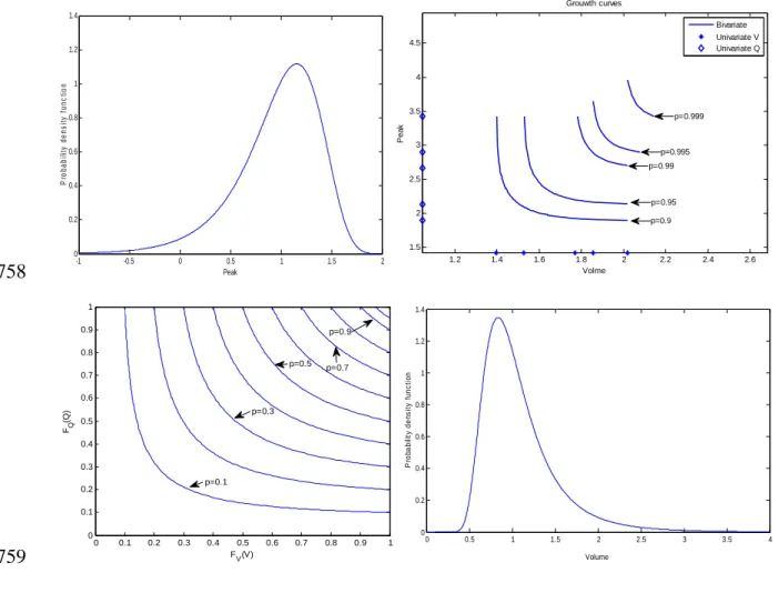
The bivariate regional growth curve is estimated for each risk value p by (12) and by 442
using the regional parameters of the bivariate distribution. On the other hand, univariate 443
regional growth curves of V and Q are estimated directly using regional parameters of 444
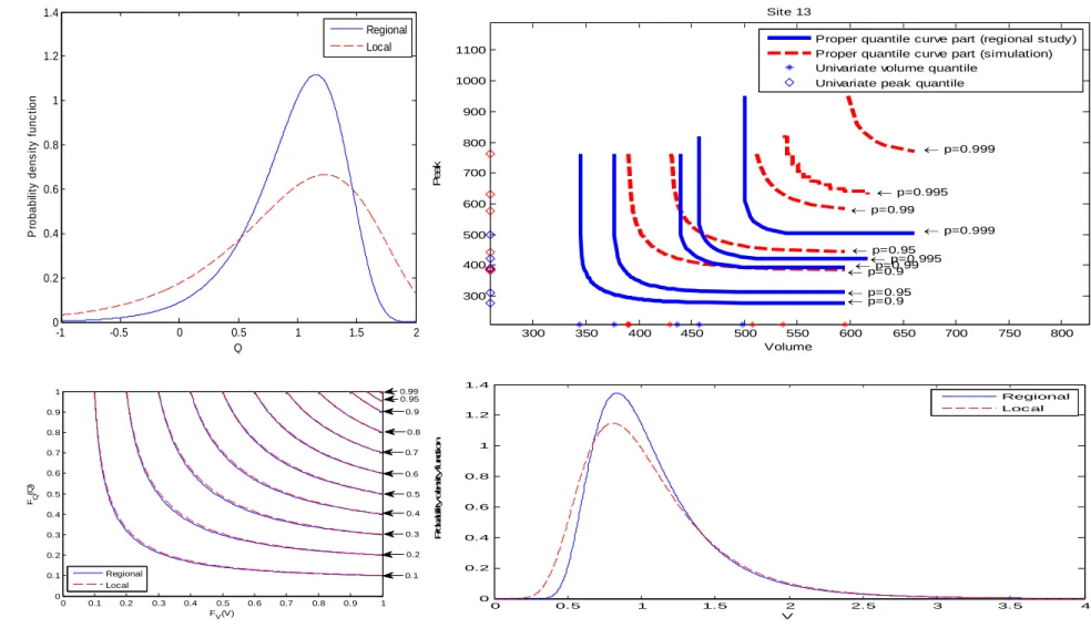
marginal distributions. Figure 5 shows the univariate and bivariate estimated growth 445
curves corresponding to nonexceedance probabilities p =0.9, 0.95, 0.99, 0.995 and 0.999 446
as well as the quantile curve in the unit square and the marginal distributions for Q and V. 447
Univariate regional growth curves of V and Q are also presented in Table 6. Univariate 448
and bivariate quantiles can be assessed by multiplying growth curves by the 449
corresponding index flood (16). 450
24
Model performances
452
As described above, the accuracy of the quantile estimates of the three regional models: 453
univariate of V (V-model), univariate of Q (Q-model) and bivariate of (V,Q) (VQ-model) 454
is assessed using a Monte Carlo simulation procedure. The record lengths of the 455
simulated sites are assumed to be the same as those of observed data and the number of 456
simulations is set to be M=500. To illustrate these results, we present in Figure 6 the 457
univariate and bivariate quantiles of three sites derived from one simulation (M=1) and 458
from the sample data, as well as quantile curves in the unit square and the local and 459
regional marginal distributions of Q and V. Figure 6 shows that, generally, the 460
performance of the two univariate models and the bivariate model decrease with the risk 461
level and depends on the discordancy values. Indeed, for Mistassibi (Figure 6 a) the 462
performance of the V-model is higher than that of the Q-model which is in harmony with 463
the two discordance values of V and Q and with the difference between marginal 464
distributions (local and regional) of Q and V in the side panels. The performance of the 465
bivariate model depends mainly on marginal distributions. Indeed, a small difference in 466
the marginal distribution leads to possible wide shifts in the quantile curve. However, the 467
unit square curves indicate very less effect. Figure 7 illustrates the bivariate quantiles 468
(Regional and the 500 simulations) corresponding to a nonexceedance probability of 469
p=0.9 for the Petit Saguenay station. Figure 7 shows that, in the Petit Saguenay station,
470
the simulated bivariate quantile curves form a surface which includes (but not in the 471
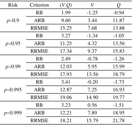
middle) the regional bivariate quantile curve. Table 7 presents the univariate and bivariate 472
model performances of the corresponding nonexceedance probability p = 0.90, 0.95, 473
25 0.99, 0.995 and 0.999. The univariate and bivariate model performances in each site are 474
presented in Figure 8. 475
Table 7 shows that the V-model performs well, since all performance criteria are less than 476
16% for all values of p. However, the performance of the Q-model is lower compared to 477
that of the V-model where for instance, for p = 0.999, the RRMSE is larger than 21%. 478
This conclusion can also be drawn from Figure 8 where the performance criteria of the Q-479
model are clearly higher than those of the V-model for all values of p. This conclusion 480
can be explained by the fact that the region is heterogeneous for Q. On the other hand, the 481
performance of the VQ-model is, generally, somewhat lower than the Q-model. This 482
conclusion is confirmed by Figure 8 where we see a close performance criteria for the 483
VQ-model and Q-model. One can explain this by the fact that the univariate quantiles are 484
special cases of bivariate quantiles, since they correspond to the extreme scenario of the 485
proper part related to the event. Then the performance of the univariate models has an 486
effect on the performance of the bivariate model. Since the performance criteria of the Q-487
model are higher than those of the V-model then effects of the Q-model performance on 488
the QV-model is more important than the effects of the V-model performance. On the 489
other hand, from Figure 8 we observe that the performance behaviour criteria of the VQ-490
model and Q-model are similar to those of Gumbel parameters (Figure 4 a), especially for 491
the scale parameter (σ). Consequently, a variation of the Gumbel parameters has an effect 492
on the Q-model performance and therefore an effect on the VQ-model performance. 493
Performance criteria corresponding to the VQ-model are less than 19% for the highest 494
considered risk level p = 0.999 (Table 7). Values of these performance criteria are larger 495
than those obtained by Chebana and Ouarda (2009). Indeed, unlike their simulation study, 496
26 the performance of the bivariate model is affected by the error of the index flood 497
estimation as well as parameter estimations. Generally the performance criteria increase 498
with the value of the risk p (Table 7 and Figure 8). An exception is recorded between 499
p=0.995 and p=0.999 where performance criteria of the VQ-model are higher for
500
p=0.995. This finding can be explained by the curse of dimensionality in the multivariate
501
context, where the central part of a distribution contains little probability mass compared 502
to the univariate framework (for more details see Scott 1992, Chebana and Ouarda 2009). 503
In order to further explain the results, we plot in Figure 9 the RRMSE of each model (for 504
p=0.99) with respect to the corresponding discordancy values. Ideally we should find an
505
increasing relation between the RRMSE of each model and the corresponding 506
discordance. This relation is observed only for the V-model (Figure 9a) since the studied 507
region is homogeneous for V, heterogeneous for Q and could be homogeneous for (V,Q). 508
To find out other factors that have an impact on the model performance, we present in 509
Figure 10 the RRMSE of the VQ-model (for p=0.99) with respect to watershed area and 510
the correlation between V and Q. Figure 10a shows that high RRMSE values are seen for 511
small watersheds whereas Figure 10b shows that sites with ρ(V,Q)> 0.6 have a good 512
performance (RRMSE of the order of 10%) with the exception of Godbout (site number 513
15) which has ρ=0.75 and high RRMSE. Godbout is one of the four sites that have a high 514
value of the Gumbel scale parameter and a high RRMSE of the Q-model and the VQ-515
model. 516
The quantile curve, for a given risk p, leads to infinite combinations of (Q,V) associated 517
to the same return period. However, they could be not equal in practice or in practical 518
point of view (Chebana and Ouarda 2011). Recently, Volpi and Fiori (2012) proposed a 519
27 methodology to identify a subset of the quantile curve according to a fixed probability 520
percentage of the events, on the basis of their probability of occurrence; see Volpi and 521
Fiori (2012) for more details. As an illustrative example, the Chamouchouane station is 522
considered. Figure 11 presents the curves and the limits with probability (1-α)=0.95. 523
5. Conclusions and perspectives
524
The procedure for regional FA in a multivariate framework is applied to a set of sites 525
from the Côte-Nord region in the northern part of the province of Quebec, Canada. This 526
procedure is proposed by Chebana and Ouarda (2009) and represents a multivariate 527
version of the index-flood model. It is based on copulas and multivariate quantiles. 528
Chebana and Ouarda (2009) evaluated the proposed model based on a simulation study. 529
In the present paper, practical aspects of this model are presented and investigated jointly 530
for the flood peak and volume of the considered data set. 531
Results show that the appropriate fitted marginal distributions are Gumbel for Q and 532
GEV for V as well as the Frank copula for their dependence structure. The multi-533
regressive proposed method to estimate the index flood is shown to lead to a high 534
performance. The performance of the two univariate models is in accordance with the 535
quality of the region (homogeneity test). Indeed, the studied region is homogenous for V 536
and heterogeneous for Q where the performance of the V-model is higher than that of the 537
Q-model. The high performance of the V-model is confirmed by a relation between their 538
performance criteria and the discordance values of V in each site whereas the low 539
performance of the Q-model is mainly caused by the variation of the marginal 540
distribution parameters. This is a logical consequence of the heterogeneity of the region 541
28 for Q. The performance of the two univariate models increases with the risk level p. For 542
the bivariate model, the performance criteria are less than 19% which indicates the high 543
performance of the proposed procedure to estimate bivariate quantiles at ungauged sites. 544
This performance increases, generally, with the risk level p and is affected by the 545
performance of the Q-model. Results show also that high values of the performance 546
criteria of the bivariate regional model are seen for small watershed and for sites with low 547
correlation between V and Q. From this study it is concluded that a good performance of 548
the bivariate model requires good performance of the two univariate models. This means 549
that we should have a homogeneous region for both univariate variables. 550
The considered method estimates the bivariate quantile as combinations that constitute 551
the quantile curve for a given risk level p. A method to select the appropriate 552
combination(s) for a specific application is of interest and should be developed in future 553
efforts. Furthermore, the adaptation of the model to the estimation of other hydrological 554
phenomena such as drought and the consideration of others homogenous regions can be 555
conducted by considering the appropriate distributions, copulas and events to be studied. 556
557 558
ACKNOWLEDGEMENTS
559
The authors thank the Natural Sciences and Engineering Research Council of Canada 560
(NSERC) and Hydro-Québec for the financial support. 561
562 563
29 564
REFERENCES 565
566
Akaike, H., 1973. "Information measures and model selection." Information measures 567
and model selection, 50: 277-290.
568
Alila, Y., 1999. "A hierarchical approach for the regionalization of precipitation annual 569
maxima in Canada." Journal of Geophysical Research D: Atmospheres, 570
104(D24): 31645-31655. 571
Alila, Y., 2000. "Regional rainfall depth-duration-frequency equations for Canada." 572
Water Resources Research, 36(7): 1767-1778.
573
Ashkar, F., 1980. Partial duration series models for flood analysis. Montreal, Qc, Canda, 574
Ecole Polytech of Montreal. 575
Ben Aissia, M. A., F. Chebana, T. B. M. J. Ouarda, L. Roy, G. Desrochers, I. Chartier 576
and É. Robichaud, 2012. "Multivariate analysis of flood characteristics in a 577
climate change context of the watershed of the Baskatong reservoir, Province of 578
Québec, Canada." Hydrological Processes, 26(1): 130-142. 579
Besag, J., 1975. "Statistical Analysis of Non-Lattice Data." Journal of the Royal 580
Statistical Society. Series D (The Statistician), 24(3): 179-195.
581
Brath, A., A. Castellarin, M. Franchini and G. Galeati, 2001. "Estimating the index flood 582
using indirect methods." Estimation de l'indice de crue par des méthods 583
indirectes, 46(3): 399-418.
584
Burn, D. H., 1990. "Evaluation of regional flood frequency analysis with a region of 585
influence approach." Water Resources Research, 26(10): 2257-2265. 586
Charpentier, A., Fermanian, J.-D., Scaillet, O., 2007. The estimation of copulas: Theory 587
and practice. New York, Risk Books. 588
Chebana, F. and T. B. M. J. Ouarda, 2007. "Multivariate L-moment homogeneity test." 589
Water Resources Research, 43.
590
Chebana, F. and T. B. M. J. Ouarda, 2009. "Index flood–based multivariate regional 591
frequency analysis." Water Resources Research, 45. 592
Chebana, F. and T. B. M. J. Ouarda, 2011. "Multivariate quantiles in hydrological 593
frequency analysis." Environmetrics, 22(1): 63-78. 594
Chebana, F., T. B. M. J. Ouarda, P. Bruneau, M. Barbet, S. E. Adlouni and M. 595
Latraverse, 2009. "Multivariate homogeneity testing in a northern case study in 596
the province of Quebec, Canada." Hydrological Processes, 23(12): 1690-1700. 597
Chernick, M. R., 2012. "The jackknife: A resampling method with connections to the 598
bootstrap." Wiley Interdisciplinary Reviews: Computational Statistics, 4(2): 224-599
226. 600
Cunnane, C. and J. E. Nash, 1971. "Bayesian estimation of frequency of hydrological 601
events." Internationa Association of Hydrological Sciences Publications, 100: 47-602
55. 603
Dalrymple, T., 1960. Flood-frequency analyses. Washington, D.C., U.S. G.P.O. 604
30 De Michele, C. and G. Salvadori, 2002. "On the derived flood frequency distribution: 605
analytical formulation and the influence of antecedent soil moisture condition." 606
Journal of Hydrology, 262(1-4): 245-258.
607
De Michele, C., G. Salvadori, M. Canossi, A. Petaccia and R. Rosso, 2005. "Bivariate 608
statistical approach to check adequacy of dam spillway." Journal of Hydrologic 609
Engineering, 10(1): 50-57.
610
Demarta, S. and A. J. McNeil, 2005. "The t copula and related copulas." International 611
Statistical Review, 73(1): 111-129.
612
Durrans, S. R. and S. Tomic, 1996. "Regionalization of low-flow frequency estimates: an 613
Alabama case study." Journal of the American Water Resources Association, 614
32(1): 23-37. 615
Genest, C., K. Ghoudi and L. Rivest, 1995. "A semiparametric estimation procedure of 616
dependence parameters in multivariate families of distributions." Biometrika, 617
82(3): 543-552. 618
Genest, C., B. Rémillard and D. Beaudoin, 2009. "Goodness-of-fit tests for copulas: A 619
review and a power study." Insurance: Mathematics and Economics, 44(2): 199-620
213. 621
Genest, C. and L.-P. Rivest, 1993. "Statistical Inference Procedures for Bivariate 622
Archimedean Copulas." Journal of the American Statistical Association, 88(423): 623
1034-1043. 624
GREHYS, 1996a. "Presentation and review of some methods for regional flood 625
frequency analysis." Journal of Hydrology, 186(1-4): 63-84. 626
GREHYS, 1996b. "Inter-comparison of regional flood frequency procedures for 627
Canadian rivers." Journal of Hydrology, 186(1-4): 85-103. 628
Grimaldi, S. and F. Serinaldi, 2006. "Asymmetric copula in multivariate flood frequency 629
analysis." Advances in Water Resources, 29(8): 1155-1167. 630
Hamza, A., T. B. M. J. Ouarda, S. R. Durrans and B. Bobée, 2001. "Development of 631
scale invariance and tail models for the regional estimation of low-flows." 632
Canadian Journal of Civil Engineering, 28(2): 291-304.
633
Hosking, J. R. M. and J. R. Wallis, 1993. "Some statistics useful in regional frequency 634
analysis." Water Resources Research, 29(2): 271-281. 635
Hosking, J. R. M. and J. R. Wallis, 1997. Regional frequency analysis : an approach 636
based on L-moments. Cambridge, Cambridge University Press. 637
Kim, G., M. J. Silvapulle and P. Silvapulle, 2007. "Comparison of semiparametric and 638
parametric methods for estimating copulas." Computational Statistics and Data 639
Analysis, 51(6): 2836-2850.
640
Kim, J.-M., Y.-S. Jung, E. Sungur, K.-H. Han, C. Park and I. Sohn, 2008. "A copula 641
method for modeling directional dependence of genes." BMC Bioinformatics, 642
9(1): 225. 643
Kojadinovic, I. and J. Yan, 2009. "A goodness-of-fit test for multivariate multiparameter 644
copulas based on multiplier central limit theorems." Statistics and Computing: 1-645
14. 646
Lee, T., R. Modarres and T. B. M. J. Ouarda, 2012. "Data based analysis of bivariate 647
copula tail dependence for drought duration and severity." Hydrological 648
Processes: in press.
31 Martins, E. S. and J. R. Stedinger, 2000. "Generalized maximum-likelihood generalized 650
extreme-value quantile estimators for hydrologic data." Water Resources 651
Research, 36(3): 737-744.
652
Meng, X. L. and D. B. Rubin, 1993. "Maximum likelihood estimation via the ecm 653
algorithm: A general framework." Biometrika, 80(2): 267-278. 654
Nelsen, R. B., 2006. An introduction to copulas. New York, Springer. 655
Nezhad, M. K., K. Chokmani, T. B. M. J. Ouarda, M. Barbet and P. Bruneau, 2010. 656
"Regional flood frequency analysis using residual kriging in physiographical 657
space." Hydrological Processes, 24(15): 2045-2055. 658
Nguyen, V.-T.-V. and G. Pandey, 1996. A new approach to regional estimation of floods 659
in Quebec. Proceedings of the 49th Annual Conference of the CWRA, Quebec 660
City, Collection Environnement de l’Université de Montréal. 661
NIST, 2013. e-Handbook of Statitical Methods.
662
http://www.itl.nist.gov/div898/handbook/pmd/section4/pmd44.htm, [accessed 663
september 2013]. 664
Ouarda, T. B. M. J., K. M. Bâ, C. Diaz-Delgado, A. Cârsteanu, K. Chokmani, H. Gingras, 665
E. Quentin, E. Trujillo and B. Bobée, 2008. "Intercomparison of regional flood 666
frequency estimation methods at ungauged sites for a Mexican case study." 667
Journal of Hydrology, 348(1–2): 40-58.
668
Ouarda, T. B. M. J., J. M. Cunderlik, A. St-Hilaire, M. Barbet, P. Bruneau and B. Bobée, 669
2006. "Data-based comparison of seasonality-based regional flood frequency 670
methods." Journal of Hydrology, 330(1-2): 329-339. 671
Ouarda, T. B. M. J., C. Girard, G. S. Cavadias and B. Bobée, 2001. "Regional flood 672
frequency estimation with canonical correlation analysis." Journal of Hydrology, 673
254(1-4): 157-173. 674
Ouarda, T. B. M. J., M. Hache, P. Bruneau and B. Bobee, 2000. "Regional flood peak and 675
volume estimation in northern Canadian basin." Journal of Cold Regions 676
Engineering, 14(4): 176-191.
677
Pilon, P. J., 1990. The Weibull distrubution applied to regional low-flow frequency 678
analysis. Regionalization in Hydrology, Ljubljana, IAHS Publ. 679
Rencher, A. C., 2003. Methods of Multivariate Analysis, John Wiley & Sons, Inc. 680
Salvadori, G., N. Carlo De Michele, T. Kottegoda and R. Rosso, 2007. Extremes in 681
Nature: An Approach Using Copula. Dordrecht, Springer, p292. 682
Schwarz, G., 1978. "Estimating the Dimension of a Model." Annals of Statistics, 6(2): 683
461-464. 684
Scott, D. W., 1992. Multivariate density estimation : theory, practice, and visualization. 685
New York, Wiley, p265. 686
Shiau, J. T., 2003. "Return period of bivariate distributed extreme hydrological events." 687
Stochastic Environmental Research and Risk Assessment, 17(1-2): 42-57.
688
Shih, J. H. and T. A. Louis, 1995. "Inferences on the association parameter in copula 689
models for bivariate survival data." Biometrics, 51(4): 1384-1399. 690
Singh, V. P., 1987. Regional flood frequency analysis. Dordrecht, D. Reidel Publishing, 691
p419.
692
Sklar, A., 1959. "Fonction de répartition à n dimensions et leurs margins." Institut 693
Statistique de l'Université de Paris, 8: 229-231.
32 Stedinger, J. R. and G. D. Tasker, 1986. "Regional Hydrologic Analysis, 2, Model-Error 695
Estimators, Estimation of Sigma and Log-Pearson Type 3 Distributions." Water 696
Resources Research, 22(10): 1487-1499.
697
Vandenberghe, S., N. E. C. Verhoest and B. De Baets, 2010. "Fitting bivariate copulas to 698
the dependence structure between storm characteristics: A detailed analysis based 699
on 105 year 10 min rainfall." Water Resources Research, 46(1): W01512. 700
Volpi, E. and A. Fiori, 2012. "Design event selectionin bivariate hydrological frequency 701
analysis." Hydrological science journal, 57(8): 1-10. 702
Wiltshire, S. E. (1987). "Statistical techniques for regional flood-frequency analysis. 703
[electronic resource]." 704
Yue, S., 2001. "A bivariate extreme value distribution applied to flood frequency 705
analysis." Nordic Hydrology, 32(1): 49-64. 706
Yue, S., T. B. M. J. Ouarda, B. Bobée, P. Legendre and P. Bruneau, 1999. "The Gumbel 707
mixed model for flood frequency analysis." Journal of Hydrology, 226(1-2): 88-708
100. 709
Zhang, L. and V. P. Singh, 2006. "Bivariate flood frequency analysis using the copula 710
method." Journal of Hydrologic Engineering, 11(2): 150-164. 711
Zhang, L. and V. P. Singh, 2007. "Trivariate Flood Frequency Analysis Using the 712
Gumbel-Hougaard Copula." Journal of Hydrologic Engineering, 12(4): 431-439. 713
714 715
33
Tables and Figures
716
Tables
717
Table 1: Discordancy statistic for each site (Chebana et al. 2009).
718 # Site name BV (Km2) ni (V,Q) correlation coefficient Discordancy statistic V Q (V,Q) 1 Petit Saguenay 729 24 0.50 0.80 0.40 1.09 2 Des Ha Ha 564 19 0.73 3.60 4.44 3.88 3 Aux Écorces 1120 34 0.5 0.16 2.42 0.69 4 Pikauba 489 34 0.34 0.89 1.16 1.22 5 Métabetchouane 2270 30 0.54 1.22 1.23 1.59 6 Petite Péribonka 1090 31 0.62 0.26 0.45 0.98 7 Chamouchouane (Ashuapmushuan) 15 300 43 0.70 0.13 0.14 0.26 8 Mistassibi 8690 39 0.52 0.32 0.78 0.88 9 Mistassini 9620 43 0.52 0.62 0.19 0.53 10 Manouane 3720 23 0.39 0.55 0.47 2.38 11 Valin 740 31 0.42 0.40 0.46 2.37 12 Ste-Marguerite 1100 21 0.48 1.50 0.55 1.30 13 DesEscoumins 779 19 0.49 1.14 1.81 1.27 14 Portneuf 2580 20 0.80 0.99 0.32 1.06 15 Godbout 1570 30 0.75 0.91 0.89 1.29 16 Aux-Pékans 3390 16 0.54 3.19 0.38 2.25 17 Tonerre 674 48 0.64 0.51 1.65 2.25 18 Magpie 7200 27 0.66 0.12 1.23 1.11 19 Romaine 13 000 48 0.68 1.62 0.48 0.57 20 Nabisipi 2060 25 0.78 1.12 0.64 0.54 21 Aguanus 5590 19 0.60 1.53 0.84 3.07 22 Natashquan 15 600 39 0.75 0.28 0.39 1.02 23 Etamamiou 2950 19 0.82 1.06 1.33 1.32 24 St Augustin 5750 14 0.73 0.62 0.67 0.92 25 St Paul 6630 25 0.73 0.31 1.35 1.11 26 Moisie 19000 39 0.65 1.16 0.32 0.54