Nabil EL LAMTI S50561
Grande Ecole Program student at HEC Paris Major: Finance
Thesis subject: Are smart beta strategies really smart? Thesis directed by Professor Jean-Charles Bertrand
June 14, 2017 Jouy-en-Josas, France
2 ABSTRACT
Investors, throughout the ages and especially in recent times, have differed widely in their investment philosophies (market timing/asset and security selection and allocation, active/passive investing, selecting a particular time horizon) as well as in their investment styles (with some favouring an overall macroeconomic analysis of the impact of trends on certain asset classes, others opting for more empirical, quantitatively driven approaches and finally those who seek to combine both quantitative and qualitative analyses in their investments strategies). However, no matter how disparate the strategies employed by these investors are, they all share the same objective: to generate as much return on their investment (as well as an excess return, or what they refer to as “alpha”) as possible all while minimizing the risk they have taken. This has led to the emergence of a wide range of investment strategies and portfolio construction methodologies amongst asset management funds. And while some strategies have thrived and survived the tests of time, financial empiricism and risk profile, others were either cast aside following their repeated failure to deliver on their promises or over-marketed and overhyped to appeal to investors. One such overly marketed strategy (or set of strategies) is smart beta.
In this thesis, we will go over the literature discussing and detailing smart beta strategies, analysing their growth and appeal over the last years as well as making the case for both the defenders and detractors of smart beta strategies. We will also attempt to conduct a quantitative exercise whereby we will compare the actual yields of smart beta ETF funds to what the academic theory suggests, ultimately leading us to a first answer to the question of whether smart beta strategies are indeed as smart as they are made to be.
Keywords: smart beta, investment strategies, returns, alpha, indexing, risk management, diversification, active management, passive management, portfolio construction, style factors, cost.
3
ACKNOWLEDGMENTS
The exercise of writing a thesis on a relatively recent concept is not an easy task and it would have been nigh impossible without the support and encouragement of the people who have helped me during these last three months.
Firstly, I would like to extend my heartfelt gratitude to Professor Jean-Charles Bertrand who not only assigned this extremely interesting subject, but also provided me with detailed guidance, reference articles to use for my research and took the time off from his extremely busy schedule at HSBC to thoroughly review each draft version I have sent him. Thanks to his guidance, I had fun writing this paper, despite the challenge it presented.
Secondly, I would like to thank Professor Olivier Bossard for his quick introductory session to Bloomberg. Having not interned/worked in a finance role before, I was not exposed to this tool and, as I worked on my thesis and needed data for the empirical exercise, I needed to learn the basics of using Bloomberg. Furthemore, his “Empirical Methods in Finance” class was absolutely instrumental in designing the risk analysis segment of the empirical exercise showcased in this paper.
Finally, I would like to express my eternal gratitude to my family, for their patience and their understanding (especially during periods when I neglected to call them because I was extremely busy with coursework, interviews and researching for my thesis). I would like to particularly thank my mother who had gone to extremely great lengths (and her own personal expense) to make me into the man I am today.
4 Glossary of the main terms used in this paper:
This section provides a brief definition of some of the major terms that will be utilized throughout this paper, with the aim of providing the reader with a first, basic understanding of their meaning in order for him to fully appreciate the concepts and ideas discussed in the paper.
Active fund management: Refers to a style of fund management where the human element is preponderant (i.e. having a manager or a team of managers to manage a fund’s portfolio). This style of management places heavy emphasis on the manager’s own judgement, business acumen and experience (in addition to empirical research and analysis) in making investment decisions. It is the opposite of passive fund management (also called index fund management).
Back-testing: Refers to the process of testing of an investment strategy on historical data in order to ascertain its viability before the investor actually invests capital in it. The main outcomes looked for in this process are returns and risks. The outcomes then serve as a benchmark to the investor of what his/her future yield will be if the back-tested strategy were to be applied in a timeframe similar to the one in which it was tested.
Bandwagon effect: Also called “herd mentality”, this refers to a psychological phenomenon whereby individuals perform certain actions as a result of other people doing them, irrelevant of their own beliefs. This is primarily seen in consumer behaviour (through the emergence of fads), in politics as well as in finance (especially during bull markets and asset bubble growth periods). Behavioural finance: Refers to branch of finance which seeks to explain market anomalies by studying the inherent behavioural characteristics of market participants.
Book value: Refers to the value at which an asset is recognized in a balance sheet. Calculation methodologies differ whether we refer to a single asset (in which case, its book value is equal to the cost of the asset minus the accumulated depreciation) or a company (in which case, its book value is equal to its total assets minus its intangibles and its liabilities).
Bull market: Refers to a state of the financial market whose securities’ prices are either increasing or expected to increase. It is the opposite of a bear market, where securities’ prices are either decreasing or expected to decrease, reflecting a state of pessimism from investors.
Exchange Traded Funds (ETF): Refers to a financial security which exhibits traits of an index fund, in that it tracks the performance of a benchmark index, commodity or a basket of assets. However, it can also be traded on a stock exchange like any other common stock, unlike mutual funds. As a result, ETFs experience price fluctuations on a daily basis and thus do not have a daily net asset value calculated.
Expense ratio: Refers to the measure of the cost incurred by an investment company to manage a mutual fund. It is annually calculated by taking the fund’s overall operating expenses and dividing them by the average dollar value of the fund’s assets under management.
Fundamental analysis: Refers to the analysis conducted in order to evaluate the intrinsic value of a given security by analysing several macroeconomic (economy state, industry growth), microeconomic (firm management, culture, financial state), financial, quantitative and qualitative factors. The intrinsic value obtained is then compared to the security’s current price within the market which then allows an investor to judge whether the security is over or under-priced.
5
Growth stocks: Also called “glamour stocks”, this refers to a share of a company whose growth prospects are or are expected to be above those of the market. These stocks do not usually pay a dividend as the companies that issue them usually reinvest their earnings in capital projects, thereby making them risky to an investor. An example of growth stocks is technological companies due to their nigh endless potential for innovation and advancement.
Index fund: Also called a “passively managed fund”, this refers to a category of funds that are linked to (or indexed to) a stock index such as the S&P 500 and, therefore, do not require a manager. This is in stark contrast to “actively managed funds” where the managed portfolio is composed of stocks handpicked and managed by an investment manager.
Index investing: Refers to a form of passive investing whose objective is to achieve the same level of return as a benchmark market index. This is usually done through investment in an index fund or an exchange-traded fund which track and replicate the performance of the benchmark.
Information ratio: Also called “appraisal ratio”, this refers to the ratio of the excess return of a portfolio relative to a benchmark to the standard deviation (volatility) of that return. It is used as a measure of a fund manager’s performance in generating excess returns, with the higher the information ratio, the better the performance. It is calculated using the following formula:
𝐼𝑛𝑓𝑜𝑟𝑚𝑎𝑡𝑖𝑜𝑛 𝑟𝑎𝑡𝑖𝑜 (𝐼𝑅) = 𝐸(𝑅𝑝− 𝑅𝑏) √𝑉𝑎𝑟(𝑅𝑝− 𝑅𝐵)
Leverage: Refers to the level of debt a company has taken on in order to finance its assets and operations. A company is said to be highly leveraged if its level of debt greatly exceeds its total equity value.
Liquidity: From an accounting standpoint, a company’s liquidity refers to its ability to meet its financial obligations and liabilities with the assets it has currently in both ownership and operation. Liquidity also refers to the ability of purchasing and selling an asset, stock or security easily and freely in a given market without significantly impacting its price.
Market efficiency: Refers to how security prices in a given market reflect all available information at a given time. Market efficiency is characterized by three forms: weak-form (where prices reflect all information in past trading), semistrong-form (where prices reflect all publicly available information) and strong-form (where prices reflect all relevant information, including private or inside information). Developed by Eugene Fama in 1970, this concept asserts that it is impossible for an investor to “beat the market” because all information is factored into the securities’ prices. Marketable securities: Refers to highly liquid financial securities that can be cheaply converted to cash. The high liquidity of these instruments has two sources: the very short maturities of these instruments (usually less than a year) and their rates which have little impact on their prices. Examples include: treasury bills, commercial papers and most money market instruments.
Mean reversion: Refers to the theory holding that prices and returns will revert to the average market or industry level. This is generally observed in stocks that have known extensive periods of sustained growth (usually over the span of several months or years) before reverting back to industry levels (sometimes in a sharp and unexpected manner).
6
Momentum: Refers to how quickly a security’s price or trading volume increases. It is used in technical analysis to identify potential trends that can be used to help shape investment decisions. The term is derived from physics where the momentum of an object refers to the force or speed of movement.
Net Asset Value (NAV): Refers to the value per share of a given fund at a specific time. It is calculated using the following formula:
𝑁𝑒𝑡 𝑎𝑠𝑠𝑒𝑡 𝑣𝑎𝑙𝑢𝑒 = 𝑡𝑜𝑡𝑎𝑙 𝑎𝑠𝑠𝑒𝑡𝑠 − 𝑡𝑜𝑡𝑎𝑙 𝑙𝑖𝑎𝑏𝑖𝑙𝑖𝑡𝑖𝑒𝑠 𝑛𝑢𝑚𝑏𝑒𝑟 𝑜𝑓 𝑠ℎ𝑎𝑟𝑒𝑠 𝑜𝑢𝑡𝑠𝑡𝑎𝑛𝑑𝑖𝑛𝑔
Price-to-book value ratio (P/BV): Also called the “price-equity ratio”, it refers to the ratio of the stock’s market value to its book value. It is calculated using the following formula:
𝑃 𝐵𝑉 =
𝐶𝑙𝑜𝑠𝑖𝑛𝑔 𝑝𝑟𝑖𝑐𝑒 𝑜𝑓 𝑡ℎ𝑒 𝑠𝑡𝑜𝑐𝑘
𝑇𝑜𝑡𝑎𝑙 𝑎𝑠𝑠𝑒𝑡𝑠 − (𝐼𝑛𝑡𝑎𝑛𝑔𝑖𝑏𝑙𝑒𝑠 + 𝑇𝑜𝑡𝑎𝑙 𝑙𝑖𝑎𝑏𝑖𝑙𝑖𝑡𝑖𝑒𝑠)
The P/BV ratio has various interpretations, the main ones being whether a stock is over or under-priced (signalling also the company’s overall perception by the market) or whether an investor is overpaying for a company if it were to go bankrupt immediately.
Price-to-earnings ratio (P/E): Refers to the ratio of a company’s current share price to its earnings per share. It is calculated using the following formula:
𝑃 𝐸 =
𝐶𝑢𝑟𝑟𝑒𝑛𝑡 𝑠ℎ𝑎𝑟𝑒 𝑝𝑟𝑖𝑐𝑒 𝐸𝑎𝑟𝑛𝑖𝑛𝑔𝑠 𝑝𝑒𝑟 𝑠ℎ𝑎𝑟𝑒
The P/E ratio is interpreted as the dollar amount an investor needs to invest in order to receive one dollar of the company’s earnings.
Risk-free rate: Refers to the rate of return of a zero-risk investment. This is, in practice, impossible as even the safest investments have a small amount of risk. For U.S. based investors, the three-month U.S Treasury bill is used as a proxy for the risk free rate.
Risk premium: Refers to the excess return relative to the risk-free rate of a given investment. This risk premium reflects the compensation that investors obtain from taking on more risk compared to investing in a risk-free asset.
Sharpe ratio: Refers to a risk-adjusted return measure developed by Sharpe which takes the ex-ante excess return of a given portfolio and divides it by its standard deviation. It is calculated using the following formula:
𝑆ℎ𝑎𝑟𝑝𝑒 𝑟𝑎𝑡𝑖𝑜 = 𝐸(𝑅𝑝− 𝑟𝑓) √𝑉𝑎𝑟(𝑅𝑝− 𝑟𝑓)
Short selling: Refers to the act of selling a security that is either not owned or borrowed. It is utilised as a speculative tool or a hedging tool against downward movements for the same security or a related one.
7
Technical analysis: Refers to the analysis performed in order to determine a value for securities as well as predict their future momentum. Unlike fundamental analysis which utilizes several quantitative and qualitative factors, technical analysis uses primarily statistical tools and chart analysis to forecast and evaluate a stock’s momentum and value.
Tracking error: Refers to the standard deviation of the difference of returns between the portfolio and its benchmark. There are two variants: ex-post tracking error, which is calculated on the basis of realized returns, and ex-ante tracking error, which is calculated on the basis of expected returns. Value stocks: Refers to a stock which is undervalued compared to its fundamental characteristics (such as earnings, dividends and so on). These stocks are characterised by a high dividend yield and either a low P/BV ratio or a low P/E ratio.
8
TABLE OF CONTENTS
1. Introduction 09
1.1. Motivation 09
1.2. Academic literature on smart beta strategies 09
1.3. Structure, methodology and sources used 09
1.4. Issues and challenges 10
2. Financial and economic concepts review 12
2.1. The Capital Asset Pricing Model (CAPM) 12
2.2. The Fama-French Three-Factor model 14
2.3. The Carhart Four-Factor model 15
2.4. The Fama-French Five-Factor model 16
2.5. Fundamentals of factor investing 18
3. Understanding smart beta strategies 20
3.1. Smart Beta – A tentative definition 20
3.2. Overview of the Smart Beta market 21
- The smart beta market in the U.S 22
- The smart beta market in Europe 25
3.3. Appraisal of smart beta strategies 28
- Overview of the main smart beta strategies 28
- Fundamental indexing strategies 28
- Risk-based indexation strategies 29
- Strategy/factor based strategies 32
- Making the case for smart beta strategies – literature review 33
- The case against smart beta 33
- The case for smart beta 37
3.4. First answer to the question “is smart beta really smart?” 44 4. Analysis – Performance and risks of European Smart Beta ETFs 46
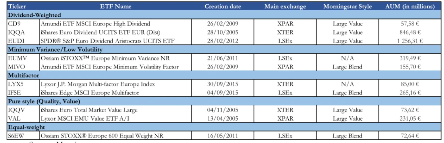
4.1. Universe selection and methodology 46
4.1.1. Dividend-weighted ETFs mini factsheets 47
4.1.2. Minimum variance/Low Volatility ETFs mini factsheets 49
4.1.3. Multifactor ETFs mini factsheets 50
4.1.4. Pure Style ETFs mini factsheets 52
4.1.5. Equal weighted ETF mini factsheet 53
4.1.6. Methodology 54
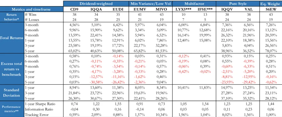
4.2. Empirical results and discussion 56
4.2.1 Portfolio performance analysis 56
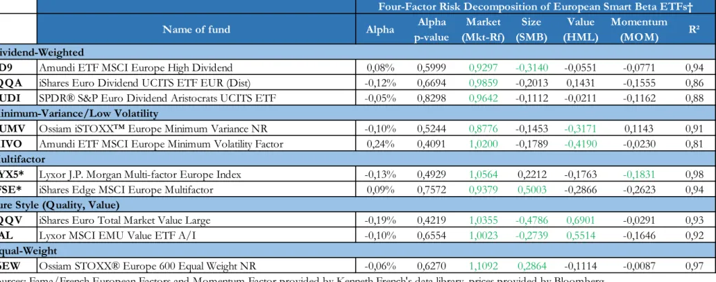
4.2.2 Risk factor decomposition analysis 62
4.3. Performance and risks of European Smart Beta ETFs: Conclusion 66 5. Thesis conclusion: Are smart beta strategies really smart? 67
Annexes 68
List of tables and charts 73
9 1. Introduction
In this section of the paper, we will provide some insight on the motivation behind selecting “smart beta” as a thesis subject, discuss the current state of academic literature regarding it and outline the structure this paper will follow. Furthermore, we will detail the methodology and sources we intend to use as well as some issues and limitations we have encountered during the preparation of this paper.
1.1. Motivation:
The interest in studying smart beta strategies as a thesis subject stemmed from the inherent promise they offer: higher returns at lower costs and risk. Considering the current economic and financial situation, as well as factoring in the resulting monetary policies, this promise appears to be not only too good to be true, but also seems to be attracting more and more investors.
The observed growth in smart beta launches over the recent years does seem to give credence to the above-mentioned promise with the United States leading the pack and Europe slowly catching up. However, as smart beta strategies continue to get over-marketed and overhyped, many researchers, economists and scholars have made the case against them, calling them unsustainable, a temporary “fad” and even “dumb” (as in, they do not yield the high returns they promise through some breakthrough asset selection process but rather through very risky means and by considering certain punctual idiosyncrasies that may not be replicated in the long term, in contrast to the whole “smart beta” label they carry). Charles Aram, the head of the Research Affiliates EMEA branch, has put the researchers’ fears and doubts in a much blunter manner. In the September 2016 issue of Fund Strategy, he states that: “If something [referencing smart beta strategies] has been “hot” recently, it risks performing badly […] If you overpay, no matter what the quality of the asset, you get a poor investment result. Investors need to look before they leap”. Such a statement raises concerns regarding investors’ behaviour towards this new concept as well as beg the question that lends this thesis its namesake “are smart beta strategies really smart?”. It is a question that poses an interesting challenge and we will attempt to provide an answer to it in what will follow, to the best of our abilities.
1.2. Academic literature on smart beta strategies:
Smart beta strategies, as they are denominated, are still considered a new concept and, thus, academic research on smart beta strategies is scarce. However, considering that smart beta strategies exhibit characteristics of both active and passive fund management, some economists, fund managers, investors and researchers have leveraged the existing literature regarding them to begin analysing and understanding how smart beta strategies operate and how they contribute in terms of both risk and return to the average investor’s portfolio.
As we will see in the “methodology” section, we will only limit ourselves to using research and academic papers that specifically discuss smart beta strategies, all while providing a small refresher on certain relevant economic theories and the basic characteristics of both active and passive fund management. This is done so as to help the reader in his/her understand of the subject and to encourage further research on it.
1.3. Structure, methodology and sources used
The thesis aims at providing a first answer to the question of whether smart beta strategies are truly “smart”. To do so, we have elected to structure the paper as follows:
10
Firstly, we will begin by providing the reader with basic definitions of certain economic concepts and theories that smart beta strategies are built upon. Such concepts include, but are not limited to, the Capital Asset Pricing Model, the concept of beta and alpha, the Fama-French Three-Factor model (and its extension, the Carhart Four-Factor model) and the main characteristics of active and passive fund management. While non-exhaustive, this section of the paper aims to prepare the reader for the discussion on smart beta strategies, to facilitate his/her understanding of the concept and to enable him/her to make their own judgement on whether smart beta strategies are indeed “smart”.
Secondly, we will introduce the concept of smart beta and proceed to a review of the relevant academic literature surrounding the concept. While smart beta does not have a universally accepted definition and is an umbrella term for various investment strategies, various definitions provided by scholars and researchers have common elements and thusly, we will provide them all while highlighting the significant differences that may arise. Regarding the academic literature review, we will limit ourselves to the relevant and most recent articles regarding smart beta, making the case for both the defendants and the detractors of the concept and summarizing their main findings and recommendations. Thirdly, we will present and summarize the findings of a quantitative exercise revolving
around smart beta funds. The aim of this objective is to determine the source of return from these funds and whether they deserve to be called “smart”. This exercise will consist mainly of a statistical analysis of the various components of the returns of these smart beta funds. The main financial data sources that will be used in this exercise are Bloomberg and Morningstar.
Finally, we will conclude with an overall summary of our findings, provide our own opinion on whether smart beta strategies are indeed smart as well as provide guidelines and further references on portfolio construction using smart beta strategies and products.
We conclude this subsection by highlighting the main sources (online and offline) of information used throughout this paper, most of which are provided by the HEC Paris library. These sources are:
The Journal of Portfolio Management The Journal of Financial Planning The Journal of Applied Finance
Various financial publications, newspapers and periodicals such as: The Financial Times, The Wall Street Journal, Fund Strategy etc…
Online financial resources and websites such as Investopedia, EDHEC Risk, Fama-French Tuck School of Business website etc…
Financial data banks such as Bloomberg and Morningstar. 1.4. Issues and challenges:
As stated above, the main challenges encountered when writing this paper were twofold:
Firstly, while articles regarding factor investing (whose concepts upon which smart beta strategies are based) are abundant, articles about smart beta as a standalone concept are rather scarce. This is due to two reasons:
o “Smart beta” is a commercial denomination coined by various funds and investors, not an academic one;
o Smart beta, as a concept, remains relatively new among investors despite, as we will see later in the paper, rapidly gaining ground.
11
Therefore, the main challenge was to wade through the massive variety of articles regarding factor investing and selecting those that are linked and relevant to smart beta strategies; Secondly, the difficulty of access to relevant financial data in order to construct the
quantitative exercise to illustrate the sources of return for smart beta funds.
Furthermore, this paper relies on carefully selected publications which reflect their authors’ opinions and, thusly, constitute in no shape or form a definitive or absolute stance on the subject. They are used as a reference to illustrate the advancements of academic research on the subject of smart beta and have been further analysed in order to highlight and compare their authors’ arguments and opinions.
Finally, we have elected to approach the financial data used in this paper with caution and scepticism, especially data coming from product providers and from certain publications. This data has been cross-checked with other data providers such as Bloomberg and Morningstar, since they are considered objective by financial experts.
12 2. Financial and economic concepts review
To fully appreciate and understand the underlying theoretical concepts behind smart beta strategies as well as the views and opinions of the academic authors that have studied them, it is important to provide the reader with a basic introduction of some of the most relevant financial and economic theories which constitute not only the backbone of smart beta strategies but are widely and commonly used in almost all financial areas of expertise. The concepts covered in this section will also help shed some light on how smart beta strategies came to exist as some of the underlying ideas in these concepts have been challenged over time and many of their weaknesses have pushed investors and asset managers alike to seek out “alternative” ways to achieve higher returns.
We will discuss five essential concepts in this section: the capital asset pricing model, the Fama-French three-factor model, its upgraded versions the Carhart four-factor model and the Fama-French five-factor model, and the fundamentals of factor investing.
2.1. The Capital Asset Pricing Model (CAPM):
Born from the work of Harry Markowitz on portfolio theory and portfolio diversification, the Capital Asset Pricing Model was introduced by William Sharpe, among others1, in 1964 in his
paper “Capital Asset Prices: A Theory of Market Equilibrium under Conditions of Risk”.
The CAPM is based on a set of assumptions that can be broken down into assumptions on the market and on its participants.
Market-wise, the CAPM assumes the following: The market does not have any intermediaries;
There are no constraints on the positions held (i.e. no constraints on borrowing or short-selling);
Supply and demand are immediately matched; There are no transaction costs.
Investor-wise, the CAPM assumes the following:
Investors all seek to maximize their portfolio’s value;
Investors are rational, risk-averse, share the same beliefs and care only about the mean and variance;
Investors have access to all available information at the same time; Investors only have a one-period investment horizon.
Under these assumptions, the CAPM provides an easy framework to understand the relationship between the return of a security/portfolio and its risk. This framework is illustrated by the following relationship:
𝐸(𝑟𝐴) = 𝑟𝑓+ 𝛽𝐴 × (𝐸(𝑟𝑀) − 𝑟𝑓) (1) Where:
𝐸(𝑟𝐴) is the expected return of the asset/portfolio;
𝑟𝑓 is the risk-free rate;
1Sharpe was not the first one to leverage upon Markowitz’s work to introduce the concept of CAPM. Treynor (1961, 1962), Lintner (1965) and Mossin (1966) have independently introduced the concept in their work. However, only Sharpe, alongside Markowitz and Merton were awarded the 1990 Nobel Memorial Prize in Economics for their work.
13
𝛽𝐴 is the measure of the risk of the security/portfolio; 𝐸(𝑟𝑀) is the expected return of the market.
When measuring risk, the CAPM uses beta as a measure which is governed by the following relationship:
𝛽𝐴 =𝐶𝑜𝑣(𝑟𝐴; 𝑟𝑀) 𝜎(𝑟𝑀)2 (2)
Where:
𝐶𝑜𝑣(𝑟𝐴; 𝑟𝑀) is the covariance of the return of security/portfolio relative to the return of
the market;
𝜎(𝑟𝑀)2 is the variance of the market return.
There are two ways to interpret the beta used in the CAPM according to Fama and French (2004:28-29):
First interpretation: According to (1), mathematically, beta can be viewed as the slope of the regression between the expected return of the security/portfolio and the market return. Thus, beta measures how sensitive the security/portfolio’s return is compared to the market return;
Second interpretation: According to (2), beta can be viewed as the risk each dollar invested in security/portfolio A contributes to the market portfolio. This is an economic interpretation that stems from observing that the risk of the market portfolio (measured by 𝜎(𝑟𝑀)2) is a weighted average of the covariance risks of the assets within the market
portfolio, thus making beta the measure of covariance risk of security/portfolio A relative to the variance of the market portfolio return. It is this interpretation that we will use throughout our paper when discussing smart beta strategies.
Furthermore, the CAPM distinguishes between two types of risk: systematic and specific. Systematic risk refers to the risk borne from the inherent market structure itself, its actors as well as any and all factors that cannot be diversified away such as monetary policy, political events, natural disasters and so on. In contrast, specific risk refers to the risk that is proper to a certain security/portfolio and, therefore, can be diversified away and hedged against. Because of this, the CAPM only reflects systematic risk through the beta measure, with the beta of the market being equal to 1, lower-risk securities/portfolios having a beta less than 1 and higher-risk securities/portfolios having a beta greater than 1.
Ultimately, the CAPM’s main message is: When investing in a given security/portfolio, investors are doubly rewarded: once, through the effect of the time value of money (which is reflected by the risk-free component of the equation (1)) and once through the effect of taking on more risk.
However, the CAPM is not an empirically solid model and owes its failure to an overly simplistic set of assumptions as well as difficulties in implementing validating tests at the time when the model was first introduced (Fama and French, 2004:25). Thus, throughout the years, the CAPM has been revisited and upgraded to not only correct its shortcomings but also to reflect the financial and economic changes of the times. Sharpe (1990:313), in his review of the CAPM, has listed several examples of amendments brought forth by many economists and financial expert to his initial model.
14 Such examples include but are not limited to:
Black, in 1972, introduced a CAPM version where no riskless asset existed;
Merton presented two amendments to the CAPM framework, one in 1973 which dealt with future investment opportunities and one in 1987 which dealt with market segmentation; Markowitz, in 1990, presented a version of the CAPM framework which addressed the
assumption on no constraints regarding short-selling.
One major review was done in 1993 by Fama and French who proposed an extension of the CAPM which adds two new factors to the market risk factor. It is this model that we will discuss in the next subsection.
2.2. The Fama-French Three-Factor model:
The Fama-French Three-Factor model was developed in 1993 by professors Eugene Fama and Kenneth French as a response to the incompleteness of the CAPM. It argues that returns from securities and portfolios are influenced by two additional factors, in addition to the market risk factor that is introduced by the CAPM: market capitalization (referred to as the “size” factor) and the book-to-market ratio (referred to as the “value” factor).
According to Fama and French, the main justification for the addition of these factors is that both size and book-to-market (BtM) ratios are linked to the economic fundamentals of the companies that issue the securities (Fama and French, 1993:7-8). They further elaborate that:
Earnings and book-to-market ratios as negatively correlated, with firms with low BtM ratios presenting consistent higher earnings than firms with high BtM ratios;
Size and average returns are negatively correlated due to a common risk factor. This stems from their observation of the evolution of earnings of small firms in the 1980s: they argue that small firms suffer longer periods of earnings depression than bigger firms should the economy in which they operate suffer from a recession. They have also observed that following the 1982 recession, smaller firms have not contributed to the economic growth of the mid and late 80s;
Profitability is not only related to size but also to BtM and is a common risk factor that highlights and explains the positive correlation between BtM ratios and average returns. As such, under the Fama-French Three-Factor model, the return of a security/portfolio becomes:
𝐸(𝑟𝐴) = 𝑟𝑓+ 𝛽𝐴 × (𝐸(𝑟𝑀) − 𝑟𝑓) + 𝛽𝑆 × 𝑆𝑀𝐵 + 𝛽𝑉 × 𝐻𝑀𝐿 + 𝛼 + 𝜖 (3) Where:
𝐸(𝑟𝐴) is the expected return of the asset/portfolio; 𝑟𝑓 is the risk-free rate;
𝛽𝐴 is the measure of the risk of the security/portfolio; 𝐸(𝑟𝑀) is the expected return of the market.
𝛽𝑆 is the measure of the risk related to the size of the security/portfolio;
𝛽𝑉 is the measure of the risk related to the value of the security/portfolio;
𝑆𝑀𝐵 (which stands for “Small Minus Big”) measures the difference in expected returns between small and big firms (in terms of market capitalization);
𝐻𝑀𝐿 (which stands for “High Minus Low”) measures the difference in expected returns between value stocks and growth stocks;
15 𝛼 is a regression intercept;
𝜖 is a measure of regression error.
Both SMB and HML are calculated by using both available historical data and a combination of portfolios that focus on size and value, respectively. These values are reported
regularly by professor French on his personal website:
http://mba.tuck.dartmouth.edu/pages/faculty/ken.french/data_library.html
Meanwhile, the betas for both the size and value factors are, alongside 𝛼, determined through linear regression and can have both positive and negative values.
The Fama-French Three-Factor model, however, is not without its shortcomings. One major issue with the model was highlighted by Griffin (2002: 786-798) where he argues that the Fama-French factors of value and size are more accurate in their explanation of return variations when applied locally as opposed to when they are applied globally. As a result, each of the factors should be considered on a per country basis (and it is currently done so on professor French’s website, where he defines SMB and HML factors of each country such as the United Kingdom, France and so on).
While the Fama-French has indeed taken a step further than the CAPM to breakdown security returns, it remains an incomplete model and the interpretation of its new factors are geographically constrained. Efforts have been made throughout the years to further complete this model, with Fama and French introducing two other factors in 2015, namely profitability and investment strategy and other researchers such as Carhart (1997), who introduced a fourth factor, momentum, to the original Three-Factor model. It is this model that we will discuss in the next subsection.
2.3. The Carhart Four-Factor model:
As stated above, Mark Carhart introduced, in 1997, an extension of the Fama-French Three Factor model (1993) by adding a new factor: momentum.
Momentum is defined as the observed tendency for prices to keep increasing further after their initial increase or to keep decreasing further after their initial decrease. The very definition of momentum makes it somewhat of an anomaly as, according to the Efficient Market Hypothesis, there is no valid reason for security prices to keep increasing or decreasing after an initial shift in their value.
While traditional financial theory fails to clearly define what truly causes momentum to appear in some securities, behavioural finance offers some insights on why momentum exists; indeed, Chan, Jegadeesh and Lakonishok (1996) argue that momentum arises from most investors’ inability to swiftly and immediately react to new information in the market and, thusly, integrate that information into security prices. This explanation highlights the irrationality of investors when it comes to their appraisal of the value of certain securities and to their investment choices.
Carhart’s motivation for integrating the momentum factor in the Fama-French Three-Factor model stems from the model being unable to explain return variation when it comes to momentum-sorted portfolios (Fama and French, 1996 – Carhart 1997). As such, Carhart leveraged on Jegadeesh and Titman’s (1993) one-year momentum variation and included it in his model.
16
Under the Carhart model, the return of a security or portfolio can be written as:
𝐸(𝑟𝐴) = 𝑟𝑓+ 𝛽𝐴 × (𝐸(𝑟𝑀) − 𝑟𝑓) + 𝛽𝑆 × 𝑆𝑀𝐵 + 𝛽𝑉 × 𝐻𝑀𝐿 + 𝛽𝑀 × 𝑈𝑀𝐷 + 𝛼
+ 𝜖 (4)
The explanations of the factors in (4) are identical to those of (3) with the addition of the following: 𝛽𝑀 is the measure of the risk related to the momentum factor of the security/portfolio; 𝑈𝑀𝐷 (which stands for “Up Minus Down”) measures the difference in expected returns
between “winning” securities and “losing” securities (in terms of momentum).
As stated by Carhart in his paper, the four-factor model can be used in the same fashion as both the CAPM and the Fama-French Three-Factor in explaining the sources of the return of a given security/portfolio (Carhart, 1997). However, the model is mainly used in asset management to assess the performance of an actively managed portfolio as well as evaluate the overall performance of a mutual fund.
In this next section, we will discuss the recently updated Fama-French model, which adds two additional factors to the original three (market, size and value) in an attempt to further explain the returns observed of any given security.
2.4. The Fama-French Five-Factor model:
In 2014, Fama and French assert that the initial three-factor model that they have developed in 1993 does not fully explain certain irregularities observed in expected returns. As a result, Fama and French upgraded the three-factor model by incorporating two additional factors, namely profitability and investment.
The rationale for these two factors stems from the theoretical implications of the dividend discount model (DDM)2 which asserts that profitability and investment further explain returns
obtained from the HML factor in the initial model.
Surprisingly, the new Fama-French model does not include the momentum factor, as opposed to the Carhart model. This is mainly due to Fama’s stance on momentum. While not disproving its existence, Fama believes that the level of risk carried by securities in an efficient market cannot change so abruptly and significantly that it justifies the need to acknowledge the momentum factor’s role in it.
Under the Fama-French five-factor model, the return of any security is given by the following equation:
𝐸(𝑟𝐴) = 𝑟𝑓+ 𝛽𝐴 × (𝐸(𝑟𝑀) − 𝑟𝑓) + 𝛽𝑆 × 𝑆𝑀𝐵 + 𝛽𝑉 × 𝐻𝑀𝐿 + 𝛽𝑃 × 𝑅𝑀𝑊 + 𝛽𝐼 × 𝐶𝑀𝐴 + 𝛼 + 𝜖 (5)
The explanations of the factors in (5) are identical to those of (3) with the addition of the following: 𝛽𝑀 is the measure of the risk related to the profitability factor of the security/portfolio; 𝑅𝑀𝑊 (which stands for “Robust Minus Weak”) measures the difference in expected
returns between securities that exhibit strong profitability levels (thus making them
2 The dividend-discount model is a method of computing a security’s price by calculating the present value of the expected dividend the underlying security’s company will pay.
17
“robust”) and securities that show inconsistent profitability levels (thus making them “weak”);
𝛽𝐼 is the measure of the risk related to the investment factor of the security/portfolio; 𝐶𝑀𝐴 (which stands for “Conservative Minus Aggressive”) measures the difference in
expected returns between securities that engage in limited investment activities (thus making them “conservative”) and securities that show high levels of investment activity (thus making them “aggressive”).
To test the new model, Fama and French constructed several portfolios that are designed to exhibit large differences in returns caused by the size, value, profitability and investment factors. They have also performed two exercises:
The first one is the regression of the returns of the portfolios constructed against the upgraded model. This was done to evaluate how much it explains the differences in returns observed in the selected portfolios;
The second one is comparing the performance of the new model versus the three-factor one. This was done to highlight whether the new five-factor model explains the discrepancies in returns noted in the original three-factor model.
Fama and French summarize their findings regarding the new model as follows:
In terms of structure, the HML factor becomes redundant as any value contribution within the return of a security can already be explained by the market, size, investment and profitability factors. Thusly, Fama and French encourage investors and academics to drop the HML factor if they are merely interested in explaining abnormal returns. However, they do advocate for the use of all five factors if the intent is to explain returns from portfolios that exhibit size, value, profitability and investment tilts;
The model also manages to explain between 69% and 93% of the return discrepancies that were noted following the use of the previous three-factor model.
However, this new model is not without its shortcomings. In their 2016 paper “Five concerns with the Five-Factor model”, Blitz, Hanauer, Vidojevic and van Vliet (henceforth known as BHVV), raised five issues with the new Fama-French five-factor model. While two of these issues are linked to some of the old factors present in the original Fama-French three factor model (mainly the continued existence within the model of the CAPM relationship between market risk and return, as well as, the overall acceptance by the academic community of the new model when some of the original factors are still being contested), some of the other issues are linked to how the model itself has been constructed. These issues being:
The absence of the momentum factor;
The lack of robustness of the new factors introduced. The concerns here are historical (i.e. will these factors be relevant for data points older than 1963) and whether these factors also work with other asset classes;
The lack of sufficient empirical justification behind the introduction of these factors from Fama and French.
In this next section, we will discuss the main concept behind factor investing, which is the use of factors that reflect the fundamentals of a given market/security and, thusly, drive any return and risk obtained from it.
18 2.5. Fundamentals of factor investing:
The premise of factor investing, as we will see when discussing smart beta strategies, is that certain strategies are built around giving more importance to certain factors than others. While many popular smart beta ETFs use traditional factors such as Fama-French’s three factors (market, size and value) as well as momentum, some strategies use exotic or more specialized factors in their construction.
The aim of this section is not to list every potential factor that exists, but offer to the reader an insight on the main existing categories of factors and how they are evaluated by researchers.
Harvey, Liu and Zhu (henceforth known as HLZ), in their 2016 paper “…and the Cross-Section of expected returns”, analysed a considerable body of literature regarding expected returns, and how academics attempt to explain them using various factors. The aim of their paper was to provide a factor evaluation model that relies on statistical thresholds. If factors, old and new, cleared those thresholds, then the factor would be deemed relevant.
To do so, HLZ reviewed 313 papers covering 316 different factors. While they deem the number of factors reviewed limited, they argue, however, that these factors are listed in papers that either have been published in respected financial publications or are currently being reviewed. The factors reviewed were classified under two main groups:
“Common” factors, which make up 36% of the factors listed, refer to factors that affect the returns of all securities/assets regardless of their inherent characteristics. Under these factors, we find market, investment, accounting standards and so on. These factors are usually referred to as “systematic” factors and their effect on returns cannot be diversified away;
“Characteristics” factors, which make up 64% of the factors listed, refer to factors that are unique to each security/asset. These factors are usually referred to as “idiosyncratic” factors and their effect on returns can be diversified away.
In terms of how to evaluate these factors, HLZ argue that because data mining has become easier and less costly than in the past, the statistical threshold (namely, the “t-statistic”) to consider any studied factor as relevant, should be raised. In statistics, the rule is that the higher the t-statistic, the higher the likelihood that the studied variable is statistically relevant.
Historically, the t-stat threshold was set to 2.0. However, HLZ suggest that any new factor introduced should have a t-stat of 3.0 to be considered viable. Furthermore, they assert that any factor that comes from a combination of previously tested factors should have a lower t-stat threshold to be considered relevant. However, HLZ point out that many of the recently discovered factors are false discoveries and that investors should only limit themselves to an extremely reduced number of factors, especially those that have withstood the test of time and empiricism.
In summary, the abovementioned concepts should provide the reader of this paper with a first understanding of the main financial theories used in many investment strategies in general, and in smart beta, in particular. We have elected to keep the definitions of these concepts brief and to focus on the main messages and some of their relevant shortcomings so as not to deviate from the main subject of this paper. We encourage the reader to refer to the “References” section of this paper, should he/she want to explore the abovementioned concepts deeper.
19
In what follows, we will attempt to give a first definition of smart beta strategies, provide an overview of the smart beta “industry” as well go over some of the recent academic literature regarding it.
20 3. Understanding smart beta strategies
In this section of the paper, we will introduce the concept of smart beta to the reader. To this end, we will adopt the following three-point structure: Firstly, we will attempt to define smart beta strategies as, per Burton Malkiel, “there is no universally accepted definition of smart beta strategies” (Malkiel, 2014:127). To do so, we will draw upon various definitions of smart beta used by researchers and funds and combine them into a cohesive whole. Secondly, we will discuss the smart beta market, its characteristics (namely growth, structure and distribution across asset classes) as well as some of the big players in the market and their performance. Thirdly, we will go over the recent literature regarding smart beta strategies, discussing mainly the various smart beta strategies that exist, the appraisal of their performance by academics and investors as well as their stance on whether smart beta strategies are indeed “smart”.
3.1. Smart Beta – A tentative definition:
To help the reader reach a tentative definition of smart beta, we suggest reviewing some the definitions offered by investors and academics, identifying their commonalities and summarizing them into a usable definition.
Rob Arnott, chairman and founder of Research Affiliates, defines smart beta strategies as “approaches that can help achieve individual investment objectives by avoiding chasing what is popular and expensive” (Arnott, 2016:28). He warns, however, that the term smart beta is now being used to refer to any passive (or automated) strategy, arguing whether all of these strategies are indeed smart.
Echoing Arnott’s definition of smart beta is Burton Malkiel who asserts that the common impression of smart beta strategies amongst investors is that they allow them to achieve greater-than-market returns by using passive management strategies that involve a similar risk level to that of investing into a low-cost total stock index fund. Avoiding the pitfall Arnott warns against above, Malkiel explains that achieving these returns is done through tilting (or “flavouring”) the portfolio by using several factors such as value vs growth stocks, small vs large companies or other composite factors such as quality (which includes sales and earnings growth and low leverage levels), profitability, liquidity and dividend levels – making smart beta strategies akin to multifactor asset pricing models – all while not increasing the overall volatility of the portfolio and keeping the fees of such a portfolio below those charged by active managers (Malkiel, 2014:127).
Kahn and Lemmon further clarify what Malkiel has stated regarding smart beta strategies by defining them as having characteristics of both active strategies (through exposure to specific factors) and passive strategies (through the transparent and rules-based approach used to build smart beta portfolios). While Malkiel listed various factors that enter the composition of smart beta oriented portfolios, Kahn and Lemmon have focused specifically on factors that have performed well historically on average and which investors believe they will continue to do so. These factors being: value, momentum, size (with a focus on small caps), quality and volatility (mainly low-volatility/low-beta stocks). However, Kahn and Lemmon do warn that these factors, while they have performed well on average historically, have underperformed significantly over certain three- to five-year periods due to mean reversion. (Kahn and Lemmon, 2015:76).
From the above definitions, we can clearly see that there are three similarities in the definitions of smart beta suggested by academics and investors and reviewed above:
Firstly, the premise of smart beta is to achieve higher returns than a benchmark market index, all while maintaining a risk level that is similar or lower to it as well as lower fees;
21
Secondly, smart beta strategies are rule-based and focus on having exposure to certain factors that have performed historically well;
Thirdly, the selected factors are all geared towards less expensive, less “popular” and less volatile stocks.
It is also important to highlight that the term “smart beta” may refer to not only the strategies that are implemented in given portfolios, but also to indices and to some specialized funds called exchange-traded funds or ETFs which are, at the most basic level, investment funds that are traded similarly to stocks on a stock exchange. ETFs may hold several asset classes such as stocks, commodities, bonds and so on and have several advantages over traditional funds such as: lower costs, flexible buying and selling conditions, transparency and ease of diversification. It is these conditions that make ETFs suitable platforms for smart beta strategies to be applied and for smart beta portfolios to be traded.
Thusly, taking into account the similarities between the definitions discussed above as well as the fact that smart beta strategies are usually applied in exchange-traded funds, we are able to formulate our own tentative definition of what smart beta strategies are:
Smart beta strategies are a set of investment strategies that aim to achieve higher returns than a benchmark market stock all while maintaining a low level of risk and management fees. Rules-based and transparent, smart beta strategies focus on having a portfolio of stocks that are exposed to a specific set of factors that have performed well historically on average, with the most popular ones being value, size, quality and volatility. Smart beta strategies are applied within specific funds called exchange-traded funds, with certain ETFs being entirely composed of smart beta portfolios. However, smart beta strategies are also prone to periods of underperformance, mainly due to mean reversion, meaning that investors have to be wary about market timing whenever they wish to implement smart beta strategies.
Now that we have defined the term “smart beta”, in the next section, we will turn our attention to the smart beta market.
3.2. Overview of the Smart Beta market:
The purpose of this section is to provide the reader with a complete overview of the smart beta market, focusing on five characteristics: size, growth, main players, factors used and fees. While we will begin the section with describing the state of the worldwide smart beta market, we will later focus on the US and European markets since they both represent the largest and second-largest markets respectively.
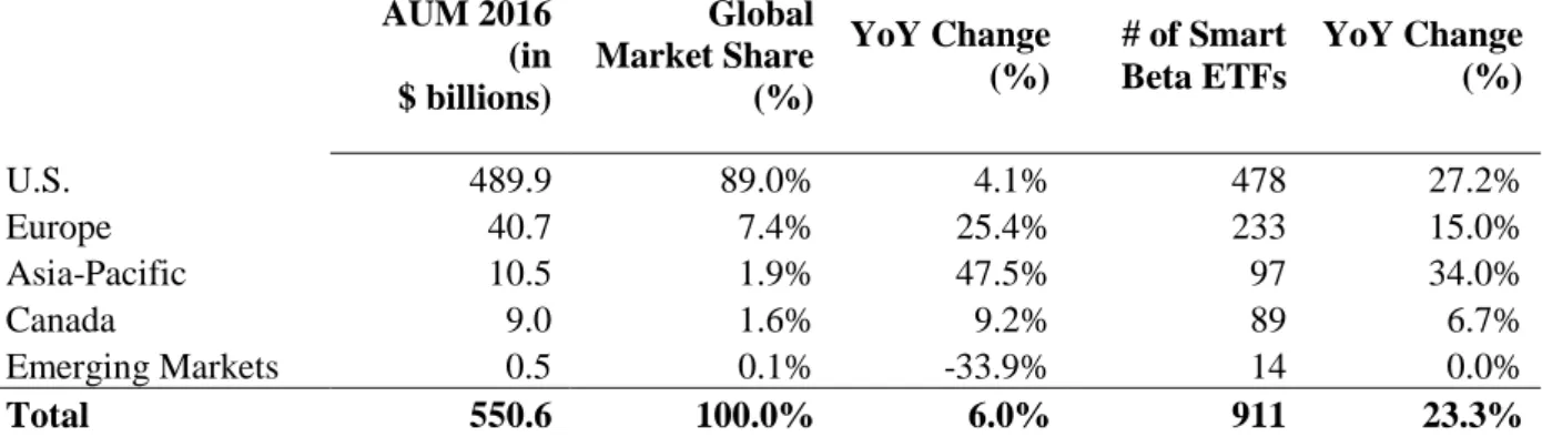
According to Morningstar, the size of the global smart beta market is roughly $550.5 billion in assets under management and 1,123 smart beta ETFs as of June 30, 2016. The main leading markets are the US (89% market share) and Europe (7.4% market share), however, in terms of growth, both European and Asian-Pacific markets have experienced significant growth compared to the other markets, with a YoY change in assets under management of 25.4% and 47.5% respectively. The table below summarizes the various findings regarding the global smart beta market:
22
Table 1: Global smart beta market figures as of June 30th, 2016.
AUM 2016 (in $ billions) Global Market Share (%) YoY Change (%) # of Smart Beta ETFs YoY Change (%) U.S. 489.9 89.0% 4.1% 478 27.2% Europe 40.7 7.4% 25.4% 233 15.0% Asia-Pacific 10.5 1.9% 47.5% 97 34.0% Canada 9.0 1.6% 9.2% 89 6.7% Emerging Markets 0.5 0.1% -33.9% 14 0.0% Total 550.6 100.0% 6.0% 911 23.3%
Source: Morningstar, A Global Guide to Strategic-Beta Exchange-Traded Products (30/09/16) AUM = Assets Under Management
Since both the United States and Europe are the largest markets with respect to smart beta ETFs, we will focus on providing insights on these two markets in what follows.
The smart beta market in the U.S:
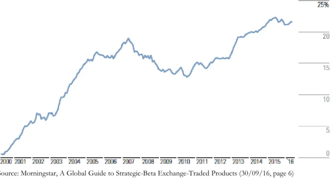
The U.S Smart Beta market is the oldest and the most mature market worldwide, with over 478 smart beta ETFs (54% of the total smart beta ETFs worldwide) and approximately $490 billion in assets under management. Smart Beta ETFs first appeared in May 2000 with both iShares Russell 1000 Growth IWF and iShares Russell 1000 Value IWD being the first and largest smart beta ETFs at the time. Since then, the U.S smart beta ETF market has been growing by leaps and bounds, not only in terms of assets under management but also in regards to its market share in the U.S ETF market, reaching almost 21% as of June 30th, 2016. The following graphs illustrate the growth of
smart beta ETFs in the U.S:
Chart 1: Evolution of U.S Smart Beta ETFs assets under management as of June 30th, 2016.
23
Strategy AUM ($ billion) % of AUM Strategy AUM ($ billion) % of AUM
Dividend-weighted 132.1 27.0% Nontraditional fixed income 7.3 1.5%
Value 108.8 22.2% Quality 4.4 0.9%
Growth 108.1 22.1% Earnings-weighted 2.6 0.5%
Low-volatility/Minimum-variance 38.6 7.9% Multiasset 1.6 0.3% Equal weight 27.6 5.6% Buyback/Shareholder Yield 1.6 0.3%
Multifactor 26.1 5.3% Revenue-weighted 0.9 0.2%
Fundamentally weighted 11 2.2% Risk-weighted 0.3 0.1%
Nontraditional commodity 9.5 1.9% Expected returns 0.2 0.0%
Momentum 9 1.8% Low/High Beta 0.1 0.0%
Chart 2: U.S Smart Beta ETFs market share evolution in the U.S ETF market as of June 30th, 2016.
Source: Morningstar, A Global Guide to Strategic-Beta Exchange-Traded Products (30/09/16, page 6)
The surprising growth of smart beta ETFs in the U.S. is mainly attributed to new investors adopting smart beta strategies as a result of the current economic situation (where low interest rates and a seven-year post-crisis bullish market have made significant returns all but impossible). Quantitatively, the smart beta ETF growth in U.S. is broken down into growth due to net new inflows since May 2000 (representing 79%) and asset appreciation (representing 21%).
Factors-wise, smart beta ETFs offering exposure to standard and simple factors (such as value, growth, dividends and low-volatility/minimum-variance) dominate the market and represent 71% of the U.S smart beta ETFs total assets under management. Dividend-weighted strategies are especially popular amongst U.S. investors for reasons mentioned above, representing 27% of the total smart beta ETFs assets under management. The following table provides a breakdown of the smart beta factors used in the U.S:
Table 2: Breakdown of U.S. smart beta factors used as of June 30th, 2016.
Source: Morningstar, A Global Guide to Strategic-Beta Exchange-Traded Products (30/09/16, page 8)
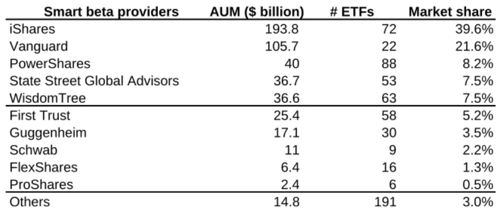
In terms of providers, iShares and Vanguard dominate the U.S. smart beta ETF providers with a 61.1% of the total U.S. smart beta assets under management, despite them only accounting for 15.4% in terms of number of smart beta ETFs in the U.S. Their position is a result of them providing smart beta solutions that follow the most popular strategies in the U.S. The following
24
Smart beta providers AUM ($ billion) # ETFs Market share
iShares 193.8 72 39.6%
Vanguard 105.7 22 21.6%
PowerShares 40 88 8.2%
State Street Global Advisors 36.7 53 7.5%
WisdomTree 36.6 63 7.5% First Trust 25.4 58 5.2% Guggenheim 17.1 30 3.5% Schwab 11 9 2.2% FlexShares 6.4 16 1.3% ProShares 2.4 6 0.5% Others 14.8 191 3.0%
tables list the most popular providers of smart beta strategies in the U.S but also the most prominent funds as well:
Table 3: Smart beta strategies providers in the U.S. as of June 30th, 2016.
Source: Morningstar, A Global Guide to Strategic-Beta Exchange-Traded Products (30/09/16, page 9)
Regarding smart beta ETFs, we have limited ourselves to the largest ETFs in the U.S. in terms of assets under management. Additional information provided includes the factors used in their smart beta strategies, their ticker as well as their expense ratios.
Table 4: Largest U.S. smart beta ETFs as of June 30th, 2016
Source: Morningstar, A Global Guide to Strategic-Beta Exchange-Traded Products (30/09/16, page 10)
Fees-wise, on average, smart beta ETFs are priced competitively with other ETFs in the U.S. However, Morningstar does warn investors to consider fees at a case-by-case basis since there are smart beta ETFs that price higher than their peer group, with certain outliers averaging the fees charged by active managers. This is primarily due to the benchmark that the smart beta ETF is tracking. One such example is the expense ratios for Schwab US Broad Market ETF SCHB and Schwab Fundamental US Broad Market ETF FNDB. The former uses as a benchmark the Dow Jones U.S. Broad Stock Market Index weighted by market-capitalization and has an expense ratio of 0.03%. The latter uses as a benchmark the Russell Fundamental U.S. Index and has an expense ratio of 0.32%. Both are smart beta ETFs and both come from the same provider, yet they charge differently.
Overall, while performance is indeed important and keeping in mind the initial promise of smart beta strategies, in the U.S., investors have always opted for the least expensive options and Morningstar warns investors to always assess the performance of smart beta ETFs that charge higher fees, to see if it is worth paying the extra cent.
Finally, Morningstar points out that there is a decreasing tendency in fees in the U.S. smart beta market with examples from longstanding funds that have cut their expense ratios
Smart beta ETF Ticker Inception date Smart beta factor used Expense ratio AUM ($ billions)
iShares Russell 1000 Growth IWF 22/05/2000 Growth 0.20% 29.3
iShares Russell 1000 Value IWD 22/05/2000 Value 0.20% 28.6
Vanguard Value ETF VTV 26/01/2004 Value 0.08% 21.8
Vanguard Dividend Appreciation ETF VIG 21/04/2006 Dividend-weighted 0.09% 21.6
Vanguard Growth ETF VUG 26/01/2004 Growth 0.08% 20.4
iShares Select Dividend DVY 03/11/2003 Dividend-weighted 0.39% 15.7
iShares Edge MSCI Min Vol USA USMV 18/10/2011 Low-volatility/Minimum variance 0.15% 14.6
Vanguard High Dividend Yield ETF VYM 10/11/2006 Dividend-weighted 0.09% 14.5
SPDR S&P Dividend ETF SDY 08/11/2005 Dividend-weighted 0.35% 14.0
25
(PowerShares FTSE RAFI and iShares Core) to recently launched funds such as Goldman Sachs ActiveBeta U.S. Large Cap Equity ETF GSLC, which charges a 0.09% expense ratio.
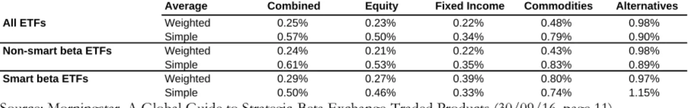
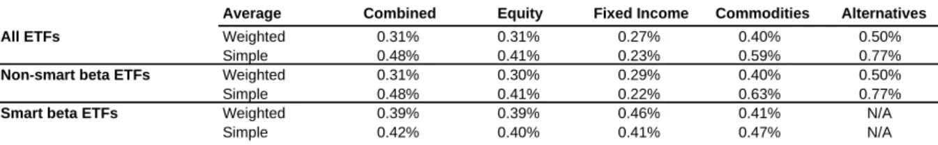
The following table provides a comparison of fees across all ETFs in the U.S., as well as across all asset classes:
Table 5: Comparative analysis of fees charged in U.S. ETFs as of June 30th, 2016
Source: Morningstar, A Global Guide to Strategic-Beta Exchange-Traded Products (30/09/16, page 11)
We will next provide an overview of the European market in the same manner as above, especially considering that the European smart beta market has been one of the fastest growing markets in recent years.
The smart beta market in Europe:
The European smart beta ETF market is relatively younger than its American counterpart. Having been established in late 2005, it is now counts 268 smart beta ETFs and is valued at $40 billion in assets under management as of June 30th, 2016 (a 25% increase compared to last year’s
AUM figures and a four-times increase overall in four years). These figures make Europe the second fastest growing smart beta ETF market in the world, right behind the Asian-Pacific market. Chart 3: Evolution of European Smart Beta ETFs assets under management as of June 30th, 2016.
Source: Morningstar, A Global Guide to Strategic-Beta Exchange-Traded Products (30/09/16, page 19)
Smart beta ETFs have had a rocky start in Europe, starting with a significant increase in market share between 2006 and 2007, before suddenly dropping in 2008. This is mainly attributed
Average Combined Equity Fixed Income Commodities Alternatives
Weighted 0.25% 0.23% 0.22% 0.48% 0.98% Simple 0.57% 0.50% 0.34% 0.79% 0.90% Weighted 0.24% 0.21% 0.22% 0.43% 0.98% Simple 0.61% 0.53% 0.35% 0.83% 0.89% Weighted 0.29% 0.27% 0.39% 0.80% 0.97% Simple 0.50% 0.46% 0.33% 0.74% 1.15% All ETFs
Non-smart beta ETFs
26
to the financial crisis having severely impacted high-dividend paying firms, thus having a severe effect on the performance of dividend-weighting smart beta ETFs due to investors removing their investments from them. However, from 2009 onward, smart beta ETFs have known a steady growth pace, reaching 7.5% in market share of the total ETF market in Europe, primarily due to consistent new smart beta ETFs launches and low-volatility oriented strategies gaining ground. Chart 4: European Smart Beta ETFs market share evolution in the European ETF market as of June 30th, 2016.
Source: Morningstar, A Global Guide to Strategic-Beta Exchange-Traded Products (30/09/16, page 20)
Factors-wise, while dividend-weighted smart beta ETFs remain the most popular choice amongst investor due to the low interest rate environment (peaking at 43% of the total assets under management of the European market), their AUM value has stagnated over the last couple of years and their market share has been dwindling with every passing year. However, both low-volatility/minimum-variance and multifactor strategies have steadily been gaining ground, reaching 19% (vs 13% LY) and 13% (vs 7% LY) respectively. The growth of multifactor strategies is particularly interesting as it is a result of both funds increasing their investments (in both funds and marketing) to promote these strategies as well as the general market tendency in Europe towards more complexity.
However, it is important to note that fixed income oriented strategies have remained stagnant in their growth and the number of fund closures is doubling year-over-year, reaching 23 closed funds as of June 30th, 2016. The latter is interpreted by Morningstar as a sign of market
maturity as surviving funds see their AUM increase and benefit from the approval of investors while funds that fail to draw in investors and assets have closed and will continue to do so.
Overall, factors-wise, the European smart beta ETF market is dominated by 3 main strategies that either echo the current economic environment (dividend-weighted, low-volatility) or a combination of current/future market tendencies and high marketing efforts (multifactor). Finally, it appears that the European market seems to be maturing rather rapidly, with well-performing funds thriving and others having their doors and activities unceremoniously shut down.
27
Smart beta providers AUM ($ billion) Market share
iShares 18.1 44.6% SPDR 3.8 9.4% Source 3.2 7.9% Lyxor 2.4 5.9% UBS 2.3 5.7% db X-trackers 2.6 6.4% Ossiam 2.1 5.2% Amundi 2.0 4.9% Think ETFs 0.7 1.7% Invesco 0.7 1.7% Others 2.7 6.7%
The following table summarises the various strategies used by European smart beta ETFs as of June 30th, 2016:
Table 6: Breakdown of European smart beta factors used as of June 30th, 2016.
Source: Morningstar, A Global Guide to Strategic-Beta Exchange-Traded Products (30/09/16, page 22)
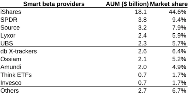
Regarding providers, iShares holds the lion’s share of the European smart beta ETF market at 44% in AUM with 70% of the largest European smart beta ETFs being provided by iShares. They are followed closely by SPDR and Source, the latter benefitting from the performance of the Goldman Sachs Equity Factor Europe ETF, a multifactor fund which has gathered around $500 million dollars in AUM as of June 30th, 2016. The following table lists the main smart beta providers
in the European market:
Table 7: Smart beta strategies providers in Europe as of June 30th, 2016.
Source: Morningstar, A Global Guide to Strategic-Beta Exchange-Traded Products (30/09/16, page 22)
Regarding smart beta ETFs, as it was the case with the American market, we have limited ourselves with the largest ETFs in Europe in terms of assets under management. Additional information provided includes the factors used in their smart beta strategies, their ticker as well as their expense ratios.
Table 8: Largest European smart beta ETFs as of June 30th, 2016
Source: Morningstar, A Global Guide to Strategic-Beta Exchange-Traded Products (30/09/16, page 23)
Strategy AUM ($ billion) % of AUM Strategy AUM ($ billion) % of AUM
Dividend-weighted 17.6 43.2% Fundamentals-weighted 0.3 0.8% Low-volatility/Minimum-variance 7.7 18.9% Momentum 0.3 0.7%
Multifactor 5.2 12.7% Growth 0.2 0.5%
Nontraditional commodity 2.9 7.2% Expected returns 0.2 0.4%
Quality 2.4 5.8% Buyback/Shareholder Yield 0.1 0.2%
Value 1.8 4.5% Multiasset 0.1 0.1%
Equal-weighted 1.3 3.2% Low/High Beta* 0 0.1%
Nontraditional fixed income 0.6 1.6% Risk-weighted* 0 0.1%
Smart beta ETF Ticker Inception date Smart beta factor used Expense ratio AUM ($ billions) iShares Developed Markets Property Yield IWF 20/10/2006 Dividend-weighted 0.59% 3.0 SPDR S&P US Dividend Aristocrats IWD 14/10/2011 Dividend-weighted 0.35% 2.3 iShares Edge S&P 500 Minimum Volatility VIG 30/11/2012 Low-volatility/Minimum variance 0.20% 2.1
iShares European Property Yield VUG 04/11/2005 Dividend-weighted 0.40% 1.6
iShares Edge MSCI World Minimum Volatility VTV 30/11/2012 Low-volatility/Minimum variance 0.30% 1.4 iShares Edge MSCI Europe Minimum Volatility DVY 30/11/2012 Low-volatility/Minimum variance 0.25% 1.2 iShares STOXX Global Sel Div 100 (DE) SDY 25/09/2009 Dividend-weighted 0.46% 1.1
iShares UK Dividend DXJ 04/11/2005 Dividend-weighted 0.40% 1.0
SPDR S&P Euro Dividend Aristocrats IVW 28/02/2012 Dividend-weighted 0.30% 0.8