HAL Id: hal-00142174
https://hal.archives-ouvertes.fr/hal-00142174
Submitted on 23 Apr 2007HAL is a multi-disciplinary open access archive for the deposit and dissemination of sci-entific research documents, whether they are pub-lished or not. The documents may come from teaching and research institutions in France or abroad, or from public or private research centers.
L’archive ouverte pluridisciplinaire HAL, est destinée au dépôt et à la diffusion de documents scientifiques de niveau recherche, publiés ou non, émanant des établissements d’enseignement et de recherche français ou étrangers, des laboratoires publics ou privés.
To cite this version:
Frédéric Bron, Dominique Jeulin. Modelling a food microstructure by random sets. Image Analysis and Stereology, International Society for Stereology, 2004, 23, pp.33-44. �hal-00142174�
MODELLING A FOOD MICROSTRUCTURE BY RANDOM SETS
F
REDERICB
RON1 ANDD
OMINIQUEJ
EULIN21Ecole des Mines de Paris, Centre des Matériaux, BP 87, 91003 Evry Cedex, France; 2Ecole des Mines de Paris, Centre de Morphologie Mathématique, 35, rue Saint-Honoré, 77305 Fontainebleau Cedex, France
e-mail: [email protected] (Accepted March 1, 2004)
ABSTRACT
Starting from scanning electron microscope images of some food products, we generate binary images of composite materials. After measuring the covariance and the probability for segments and for squares to be included in the dominant component, we develop a modelling of the microstructure from random sets obtained by thresholding Gaussian random functions. The covariance function of the underlying Gaussian random function is estimated from the experimental covariance of the food products. The validity of the model is checked by comparison of the probability curves for segments and for squares, measured on simulated and on initial images. The approach enables us to generate 3D realisations of the microstructure. Keywords: 3D simulations, food microstructure, mathematical morphology, random sets, truncated Gaussian random function.
INTRODUCTION
Some food materials represent interesting classes of composite materials. In the present study, two-phase food materials are characterised by image analysis. Then a random set modelling of the microstructure is proposed, based on image analysis measurements on 2D images.
Two dimensional scanning electron microscope (SEM) images of the food microstructures are used to make quantitative analysis of the spatial arrangements of the phases. The primary tool used in this analysis is the set covariance (also known as the two point probability function) that quantifies for a range of distances the probability that two points will both land within the phase of interest. In this study, we used a Gaussian random field model that seems capable of capturing a great deal of pertinent morphological information in a very compact manner. Once the model has been fitted, we are free to make any number of simulations (in both two and three dimensions) of
structures. We show that the set covariance and other morphological functions of the 2D and 3D simulations suit very well the experimental ones.
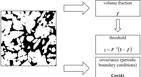
FOOD MICROSTRUCTURE
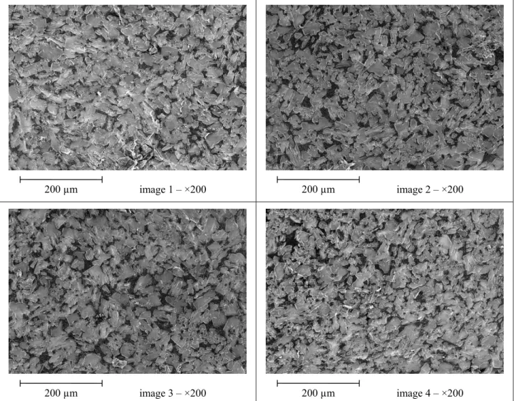
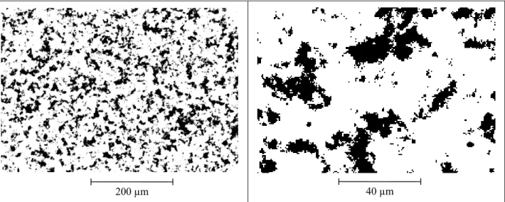
The food material studied here is a two-phase material composed of a second phase and of a matrix phase. To observe the microstructure, we used the following procedure: the samples are quickly cooled at -110 °C to congeal the microstructure and cut to observe an internal surface. Then, a projection of argon ions (Ar+) is used to etch the surface and to reveal the microstructure. Micrographs are taken with a cryogenic SEM. We based our work on four micrographs taken from the same sample (cf. Fig. 1). At the magnification used (×200), one pixel corresponds to 585 nm; the size of the images is 992×688 pixels, and the dark phase is the matrix while the bright one is the second phase.
image 1 – ×200 image 2 – ×200
image 3 – ×200 image 4 – ×200
Fig. 1. The 4 micrographs taken from the sample.
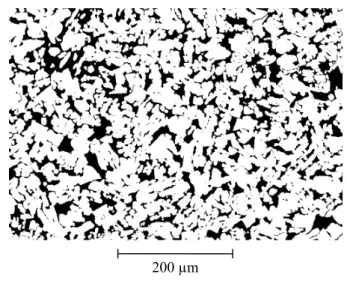
IMAGE SEGMENTATION
A difficult problem with experimental micrographs is to separate the two different phases. We need to transform grey level images into binary ones. To do this, we applied three consecutive morphological operations.
The first step is an “opening top hat”: an erosion is followed by a dilation (this is an opening). This value (one at each pixel) is then subtracted from the image so that the dark phase becomes homogeneous on the whole image. The structuring element used to perform the top hat must be larger than the cluster size, to be sure to capture the local background, but not too large if we want this operation to be useful.
For the four images, the same parameters were used: the structuring element is a hexagon with a radius of 50 pixels.
The second step is a threshold. It is selected on the histograms of the images, from the local minimum between the two peaks representing the two phases.
Finally, to remove small white dots in the black phase, a small opening by a hexagon of radius 2 pixels was performed on the binary image. The result of the segmentation for Image 2 can be seen in Fig. 2.
For each image, we can measure the volume fraction of the second phase. The mean value 75% is a good estimation for the sample. The results are given in Table 1.
200 µm 200 µm
Fig. 2. Segmentation of image 2.
MORPHOLOGICAL
MEASUREMENTS
We need to find some measurements to describe as objectively as possible the morphology of images. This is based on the theory of random sets. A random set is completely defined by probability laws generalising the case of random variables: any random closed set A is completely characterised by its Choquet capacity (Matheron, 1975; Serra, 1982; Jeulin, 1991; 2000), a functional T(K) defined over all compact sets K:
( ) (
)
(
)
( )
K
A
K
A
K
K
cQ
1
P
1
P
T
−
=
⊂
−
=
≠
∩
=
φ
(1)where P(E) refers to the probability of event E and
c
A
is the complementary set of A.In practice, different sets K are used to evaluate the morphological properties of a heterogeneous structure, but it is necessary to point out that if we cannot know the Choquet capacity for all compact sets K, we only get a limited amount of information that is not enough to identify a unique random set. It is always the case when analysing an experimental structure (Serra, 1982; 1988).
In this paper, only four different compact sets K were used: two points, a line segment, a square, or a cube. The corresponding morphological functions are explained below. Besides, we always assumed (and checked) a hypothesis of isotropy, so that each function is not dependent on the orientation; its vector argument becomes a positive real number representing a distance. We also assumed a hypothesis
of ergodicity or stationarity that allows us to replace expectations by averages over the space.
THE SET COVARIANCE
The covariance C(h) is the probability for two points A and B with a given distance h to be in the same phase ϕ.
( ) (
h A B AB h)
C =P ∈
ϕ
, ∈ϕ
, = (2)We recall here some properties of this function:
( )
( )
( )
2lim
0
0
f
h
C
C
f
h
C
h=
=
≤
≤
+∞ → (3)where f is the volume fraction of phase ϕ.
One can see on Fig. 3, the experimental covariance of the four images. They all have the same simple shape, namely a monotonically decreasing exponential function. 0.4 0.5 0.6 0.7 0.8 0 16 32 h (pix.) 48 Pdbl image 1 image 2 image 3 image 4
Fig. 3. C(h) plotted for the 4 images; at the magnification used, 1 pixel (pix.) represents 585 nm.
THE FUNCTION P
SEG( )
h
seg
P
is the probability of one line segment of a given length h to be all included in the same phase:( ) (
h
=
P
[
AB
]
⊂
,
AB
=
h
)
P
segϕ
(4)Here are some properties of this function:
( )
( )
( )
0
P
lim
0
P
P
0
seg seg seg=
=
≤
≤
+∞ →h
f
h
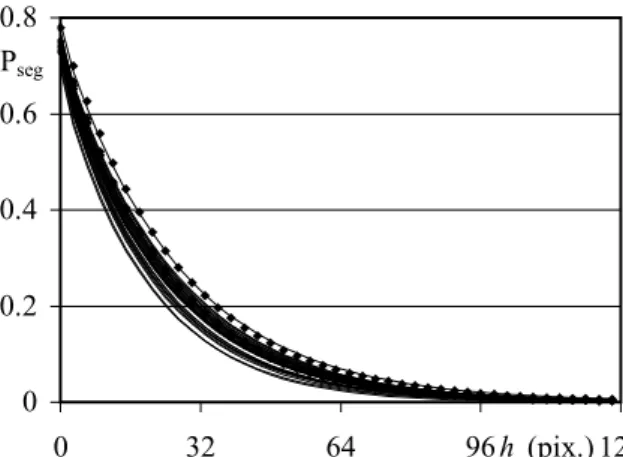
h (5)One can see on Fig. 4, the Pseg function of the four images, which can be described by a decreasing exponential function.
THE FUNCTION P
SQR( )
h
sqr
P
is the probability of one square of a given length side h to be all included in the same phase (it is related to the contact distribution function in 2D):( ) (
h
=
P
square
of
side
h
⊂
ϕ
)
P
sqr (6)Here are some properties of this function:
( )
( )
( )
0
P
lim
0
P
P
0
sqr sqr sqr=
=
≤
≤
+∞ →h
f
h
h . (7)As seen in Fig. 5, the Psqr function of the four images are decreasing exponential functions.
0 0.2 0.4 0.6 0.8 0 32 64 96h (pix.)128 Pseg image 1 images 2, 3 and 4
Fig. 4. Pseg plotted for the 4 images; 1 pixel (pix.)
represents 585 nm. 0 0.2 0.4 0.6 0.8 0 16 32 h (pix.) 48 Psqr image 1 images 2, 3 and 4
Fig. 5. Psqr plotted for the 4 images; 1 pixel (pix.)
represents 585 nm.
THE CORSON MODEL FOR THE
COVARIANCE
Corson (1974) proposed a simple model for the function C(h), called the stable covariance in the
geostatistical literature (Wackernagel, 1998; Lantuéjoul, 2002):
( )
h
(
ch
n)
C
=
α
+
β
exp
−
. (8) α and β are given by the limit conditions:( )
( )
α
β
α
=
=
∞
+
+
=
=
20
f
C
f
C
(9) So we have:( )
h
f
f
(
f
)
(
ch
n)
C
=
2+
1
−
exp
−
. (10) The parameters c and n can be obtained from a linear regression:( )
(
)
=
−
−
−
=
+
=
h
X
f
f
f
h
C
Y
nX
c
Y
ln
1
ln
ln
with
ln
2 . (11)The Corson model fits very well for the food microstructure (Fig. 6).
Table 1 gives the values of the three parameters f, c and n, the coefficient r2 and the values of h used to
apply the regression to the experimental covariance of each image and to its average. One can notice that n is very close to 1 for every image, so that the experimental covariances are nearly exponential.
In fact, the Corson model for C(h) is non physical if n ≥ 1 because the slope at the origin must be strictly negative (n ≥ 1 would produce a null slope). When the slope is infinite (n < 1), we get a fractal microstructure. When n = 1, we get:
( )
0 4 0 =−Sv < dh dC , (12)where
S
v is the specific surface area of the phase divided by the total volume (Stoyan et al., 1995).In addition, a necessary condition for a function C(h) to be the covariance of a random set is that the variogram C(0) - C(h) should satisfy the triangular inequality (Matheron, 1987). It is easy to check that this inequality is violated when 1 < n ≤ 2. When n = 1, the covariance is exponential, and is permitted for a random set. For n < 1, this point can be proved as follows: consider realisations of random sets with an exponential covariance, and with a random coefficient c following a stable distribution with parameter 0 < n < 1. The resulting (non ergodic) random set has a stable covariance with parameter n.
0.5 0.6 0.7 0.8 0 16 32 h (pix.) 48 C(h) image 1 image 4 image 2 image 3
Fig. 6. Fitting of the Corson model for C(h) of the 4 images; symbols indicate experimental values with the corresponding Corson fitted model as a smooth line.
TRUNCATED GAUSSIAN
RANDOM SET MODEL
We will try now to build a 3D structure that has the same morphology as the sample. The first step is to identify the morphology of the sample on a 2D image. This will be done with the covariance function. The second step consists in building a model of a 3D structure that has the same correlation function as the 2D images. Then, one can simulate multiple 3D structures by using this random set model. This method provides a way to reflect the variability of the morphological properties in the simulations.
We use simulations based on Gaussian random functions, following the approach proposed in (Quiblier, 1984; Berk, 1987; Teubner, 1991; Roberts and Knackstedt, 1996; Roberts and Garboczi, 1999). A wide range of truncated Gaussian random sets models is given (Lantuéjoul, 2002). In the present part, we detail the derivation of the model.
Let N be the number of dimensions of the simulation space (N = 1, 2 or 3) and let Ni be the
width of the simulation in the dimension number i. Then let Ω be the simulation field, a subset of ZN,
which is a line [0; N1 – 1] or a rectangle [0; N1 – 1]×[0; N2 – 1] or a parallelepiped rectangle [0; N1 – 1] ×[0; N2 – 1]× [0; N3 – 1]. So, we have:
[
]
∏
=−
=
Ω
N i iN
11
;
0
(13)Later, we will deal only with periodic boundary conditions. We can define the set of all translations T on the network:
∏
==
N i iN
T
1Z
(14)For example, if we are in 2D (N = 2) with N1 =
10 and N2 = 13, T is defined as follows:
(
)
{
}
{
}
−
∈
−
∈
=
=
K
K
K
K
26
13
0
13
20
10
0
10
with
,
,
2 1 2 1t
t
t
t
t
T
(15)Then, if g is a function of
r
∈
Ω
we have:( ) ( )
r t gr g T t r∈Ω∀∈ + = ∀ , , . (16)BUILDING THE SIMULATION
The principle of the simulation is to generate realisations of Gaussian random functions by convolution of Gaussian noise with a weight function. A convenient way to produce these simulations is to work in Fourier space: in that case, it is easy to generate realisations with a given experimental covariance. Other methods could be used, like the Turning Bands method (Matheron, 1973; Dietrich, 1995; Lantuéjoul, 2002), involving simulations of Gaussian random functions in a lower dimensional (like 1D) space, with an appropriate covariance derived from a model of covariance in 3D. We now describe how we build the simulation.
Table 1. Volume fraction of the second phase from the 4 images and Corson parameters for the covariance.
Image f c (h in pixels) n r2 Interval used (pix.)
1 0.7795 0.1691 0.9820 0.9999 h∈
[
1;14]
2 0.7397 0.1521 0.9984 0.9999 h∈
[
1;10]
3 0.7290 0.1406 0.9942 0.9999 h∈
[
1;19]
4 0.7501 0.1612 0.9983 0.9999 h∈
[
1;19]
Non-correlated Gaussian random field
For each point r∈Ω, we define a random variable U(r), which is a standard Gaussian with null expectation and unit variance:( )
~( )
0;1 ,U r N r∈Ω∀ (17)
Because this Gaussian random field is noncorrelated:
( )
( )
( )
(
)
[
;
]
0
Cov
t
independen
are
and
,
,
2 1 2 1 2 1 2 1=
⇒
⇒
≠
Ω
∈
∀
r
U
r
U
r
U
r
U
r
r
r
r
(18) where(
X;Y)
E[
(
X E( )
X)
(
Y E( )
Y)
]
Cov = − − (19)The non-correlated Gaussian random field U can be easily generated by a computer and is the starting point of every simulation.
Introducing a correlation
In order to model a realistic microstructure, a correlation is imposed by the convolution with a weight function w (defined on Ω):
( ) (
)( )
∑
( ) (
)
Ω ∈−
×
=
=
Ω
∈
∀
hh
r
U
h
w
r
U
w
r
Z
r
,
*
(20)There are two conditions on w that will help us to give an interpretation later:
( )
( )
( )
= − Ω ∈ ∀ =∑
Ω ∈ (symmetry) , tion) (normalisa 1 2 r w r w r h w r (21)Thresholding
Finally, the correlated Gaussian field Z is thresholded to get the binary simulation B:
( )
{ ( ) }( )
( )
r
z
Z
z
r
Z
r
B
Zr z<
≥
=
≥if
,
0
if
,
1
1
(22)INTERPRETATION
Threshold z
Recall that f is the volume fraction of the phase 1 in the simulation:
( )
(
B r)
[
B( )
r]
(
Z( )
r z)
f =P =1 =E =P ≥ (23)
( )
rZ is Gaussian, as a sum of Gaussian variables (by construction, it is also standard):
( )
~( )
0,1 ,Z r N r∈Ω ∀ (24) and then( )
(
)
(
( )
)
( )
(
f
)
F
z
z
F
z
N
z
N
f
−
=
−
=
<
−
=
≥
=
−1
1
1
,
0
P
1
1
,
0
P
1 (25)where F is the cumulative distribution function of a standard Gaussian.
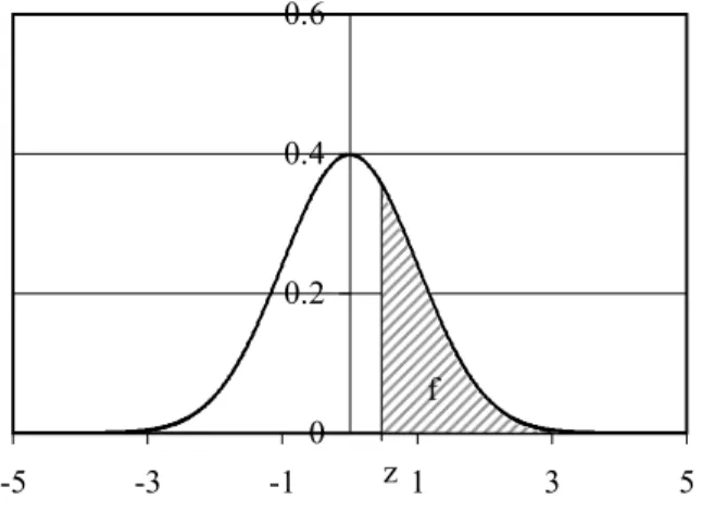
This gives a simple interpretation of the threshold z: the volume fraction f is the probability of a standard Gaussian to be greater or equal to the threshold z (see Fig. 7).
0 0.2 0.4 0.6 -5 -3 -1 1 3 5 f z
Fig. 7. Interpretation of the threshold z.
Weight function w
To understand better the meaning of w, we need to calculate the covariance of Z
( )
r andZ(
r+h)
. It is easy to show that we have:( ) (
)
[
Z r ,Z r h]
(
w*w)( )
hCov + = (26)
where * is the product of convolution, with
( ) (
)
[
Z r ,Z r+h]
=ρ( )
h Cov . (27) And so now:( ) (
)( )
( )
( )
w
( )
w
h
w
w
h
FFT
FFT
FFT
*
×
=
ρ
=
ρ
(28) where FFT means the fast Fourier transform (a discrete Fourier transform). The imaginary part of( )
wFFT is null because of the symmetry of w. So
( )
ρFFT is a real positive and:
( )
(
ρ)
=FFT−1 FFT
The covariance ρ is related to the covariance of the binary images, defined by thresholding the Gaussian random function. This is done through the bivariate Gaussian distribution:
(
)
(
2)
2 1 2 2 2 1 1 2 2 2 2 1 2 1 2 1 , , −ρ ρ − + − ρ − π = ρ z z z z e z z g . (30)It can be shown (Berk, 1987; Teubner, 1991; Lantuéjoul, 2002) that we have:
( ) (
)
[
]
(
)
(
)
∫
∫
∫ ∫
ρ ρ ∞ + +∞−
+
−
π
=
=
−
ρ
=
+
0 2 2 0 2 2 2 1 2 1 21
1
exp
2
1
,
,
,
,
,
Cov
t
dt
t
z
dt
t
z
z
g
f
dz
dz
z
z
g
h
r
B
r
B
z z (31)The inversion of Eq. 31 will give ρ(h). Then, we can calculate w by 29, convolve it with a Gaussian random field and threshold.
COMPUTING THE MODEL
The measurements and simulations programs follow the different steps of the model:
1. calculation of volume fraction and experimental centred covariance with periodic boundary conditions; 2. calculation of ρ(h);
3. calculation of w;
4. simulation of a non-correlated Gaussian random field 5. convolution;
6. threshold.
Experimental centred covariance with
periodic boundary conditions
With periodic boundary conditions, we have:
( )
(
( ) (
)
)
( ) (
)
( ) (
)
( )
( )
(
B B)( )
h N N r B r B r h B r B N N h r B r B N N h r B r B h r r − ′ = − = ′ − − ′ = + = + =∑
∑
Ω ∈ Ω ∈ * 1 e wher 1 1 E Cov 2 1 2 1 2 1 . (32)This expression is symmetric in h, and then (e.g. Marcotte, 1996):
( )
(
( ) (
)
)
(
)( )
( )
( )
(
)
( )
( )
(
)
x
x
B
B
N
N
B
B
N
N
h
B
B
N
N
h
r
B
r
B
h
of
conjugate
the
is
where
FFT
FFT
FFT
1
FFT
FFT
FFT
1
*
1
E
Cov
1 2 1 1 2 1 2 1×
=
′
×
=
′
=
+
=
− − . (33)This is the equation that we use to get the covariance of a given image. By construction, the experimental covariance is the inverse Fourier transform of a positive function. It is, therefore, positive definite. Then, an average over the series of images is made. The volume fraction is Cov(0).
Finally, the covariance is centred:
( )
Cov
( )
2CCov
h
=
h
−
f
. (34) If the experimental covariance is assumed to be fitted by the Corson model, we fit the model from the average on the set of images of the experimental covariance. This covariance is non-centred and without periodic boundary conditions. The first step is to calculate the non-centred covariance with periodic boundary conditions and then it is simple to centre it. This is detailed in the Appendix.Estimation of ρ(h)
Using the experimental covariance function, we estimate the covariance function ρ by inversion of the Eq. 31, for discrete values of ρ between 0 and 1 (using a set of 20000 values). The function ρ must be positive definite. To our knowledge, this is an open problem when starting from the Corson model, but in our simulations the numerical Fourier transform of ρ was positive. From the value of the volume fraction f, the threshold is calculated by 25. Another way to generate simulations is to start from a model of covariance for ρ and, then, to compute the covariance Cov(h) from Eq. 31 (Roberts and Knackstedt, 1996; Roberts, 1997; Roberts and Garboczi, 1999; Lantuéjoul, 2002). In (Wilson and Nott, 2001), a stable covariance is used for ρ, and the parameters are estimated by fitting the predicted and the experimental Cov(h).
volume fraction f covariance (periodic boundary conditions) Cov(h) threshold
(
f)
F z= −1 1−Fig. 8. Experimental structure.
B {Z z} B= 1 ≥ Z Z=w*U w U non-correlated standard gaussian random field
*
( )
(
)
(
)
(
h)
w=FFT−1 FFTρCov correlation thresholdEstimation of w and simulations
We estimate w from the Eq. 29; in fact, we need only its Fourier transform because we want to convolve it with the Gaussian white noise (Eq. 20), which is obtained by a product in the Fourier domain. Once it has been convolved, we can threshold the result to get binary images.
APPLICATION OF THE TRUNCATED
GAUSSIAN MODEL TO FOOD
PRODUCTS
Using the experimental covariance
For illustration, we made 32 (2D) simulations of the food product using the average experimental covariance. Their size is the same as the one of the experimental micrographs (992×688 pixels). Two of them are printed on Fig. 19. They look like the originals (see Fig. 2) but there is a “noise” in it: some small white dots appear in the black phase and vice versa (see Fig. 19, right). But the suitability of the simulated function C(h) to the experimental one is very good (see Fig. 10). Also we can see in Fig. 11 and Fig. 12 that the two other functions Pseg and Psqr of the simulations are very close to those from the experimental images. This is very interesting because it was not used as an input in the simulation.
0.4 0.5 0.6 0.7 0.8 0 16 32 h (pix.) 48 Pdbl
Fig. 10. C(h) for experimental images (symbols) and 2D simulations (smooth lines) using the experimental covariance. 0 0.2 0.4 0.6 0.8 0 32 64 96h (pix.)128 Pseg
Fig. 11. Pseg for experimental images (symbols) and
2D simulations (smooth lines) using the experimental covariance. 0 0.2 0.4 0.6 0.8 0 16 32 h (pix.) 48 Psqr
Fig. 12. Psqr for experimental images (symbols) and
2D simulations (smooth lines) using the experimental covariance.
Using the experimental covariance fitted
with the Corson model
For illustration, we have made 32 (2D) simulations of the food microstructure using the average experimental covariance fitted by the Corson model (last line of Table 1). Their size is the same as the one of the experimental micrographs (992×688 pixels). Two of them are printed on Fig. 20.
They look like the originals (see Fig. 2) and there is no noise as there was in the previous simulation (see Fig. 20). We have the same conclusion about the suitability of the function C(h), Pseg and Psqr but there is less variability between all the simulations.
0.4 0.5 0.6 0.7 0.8 0 16 32 h (pix.) 48 Pdbl
Fig. 13. C(h) for experimental images (symbols) and for 2D simulations (smooth lines) using fitted correlation.
0 0.2 0.4 0.6 0.8 0 32 64 96h (pix.)128 Pseg
Fig. 14. Pseg for experimental images (symbols) and for
2D simulations (smooth lines) using fitted correlation.
0 0.2 0.4 0.6 0.8 0 16 32 h (pix.) 48 Psqr
Fig. 15. Psqr experimental images (symbols) and 2D
simulations (smooth lines) using fitted correlation. The results in 3D are exactly the same as in 2D with the Corson model as the input for covariance. This enables us to generate 3D microstructures from a model estimated from 2D images. To illustrate this point, 16
(3D) simulations have been done (256×256×256). The morphological functions are shown in Fig. 16 - 18.
0.4 0.5 0.6 0.7 0.8 0 16 32 h (pix.) 48 Pdbl
Fig. 16. C(h) for experimental images (symbols) and for 3D simulations (smooth lines) using fitted correlation. 0 0.2 0.4 0.6 0.8 0 32 64 96h (pix.)128 Pseg
Fig. 17. Pseg for experimental images (symbols) and
for 3D simulations (smooth lines) using fitted correlation. 0 0.2 0.4 0.6 0.8 0 16 32 h (pixel) 48 Psqr
Fig. 18. Psqr for experimental images (symbols) and
for 3D simulations (smooth lines) using fitted correlation.
Fig. 19. 2D simulation of the food product using the experimental covariance (left), and zoom to show the artefacts.
Fig. 20. 2D simulations of the food microstructure using the experimental covariance fitted by the Corson model, and zoom in on the simulations showing that the artefacts have disappeared Fig. 20: Zoom in on the simulations to see that the artefacts have disappeared.
CONCLUSION
In this paper, we could simulate the 3D micro-structure of food products, using the truncated Gaussian model and morphological information from 2D sections.
The experimental plots of the covariance C(h) fit the model of Corson quite well (a simple monotonically decreasing exponential function).
The thresholded Gaussian random field is capable of reconstructing such a structure with the required C(h) function in both two and three dimensions. Both
visually and quantitatively, the 2D images generated from the thresholded Gaussian field agree with the 2D SEM images of the food products very well. Surprisingly, although only the covariance function is used as input to the Gaussian random field model, the simulated structures give Pseg and Psqr functions that fit the corresponding experimental functions very closely.
ACKNOWLEDGEMENT
The authors are indebted to Matthew Reed (Unilever Research) for his help and advice during the experimental part of this study.
200 µm 40 µm
APPENDIX
We offer a way to estimate a periodic covariance from an image. In two or three dimensions, h is the length of a vector.
In 1D, periodic conditions would give:
( ) (
)
(
)
(
) ( )
(
)
[
N
h
P
h
hP
N
h
]
N
h
r
B
r
B
E
dbl dbl+
−
−
=
+
1 1 11
(35) N-h r r+h r r+h r+h–N h r’ r’+(N–h)Fig. 21. Periodic boundary conditions for covariance.
The following lines prove the previous equation:
( ) (
)
(
)
( ) (
)
( ) (
)
( ) (
)
( ) (
)
( )
(
)
( ) (
)
( )
(
)
(
) ( ) ( )
(
)
(
( ) (
)
)
[
]
( )
C
(
N
h
)
N
h
h
C
N
h
N
N
N
h
r
B
r
B
h
r
B
r
B
N
h
r
B
r
B
N
h
r
B
r
B
h N r B r B h h r B r B h N N h r h N r N h N r h N r N h N r h N r N r N h r B r B h r B r B N h r B r B h r B r B−
+
−
≈
≈
+
≈
+
≈
+
+
+
≈
+
≈
+
− + + + −∑
∑
∑
∑
∑
∑
∑
− = − − = − − = − − = − − = − − = − = − + + − + + 1 1 1 1 1 0 1 0 1 1 1 0 1 1 1 0 1 1 0 1 1 E E 1 1 1 1 1 1 1 1 1 1 1 1 11
1
1
1
E
(36)We have a similar expression in 2D and in 3D.
REFERENCES
Berk NF (1987). Scattering properties of a model bicontinuous structure with a well defined length scale. Phys Rev Lett 58(25):2718-21.
Corson PB (1974). Correlation functions for predicting properties of heterogeneous materials. J App Phys 45(7):3159-64.
Dietrich CR (1995). A simple and efficient space domain implementation of the turning bands method. Water Resour Res 31:147-56.
Jeulin D (1991). Modèles morphologiques de structures aléatoires et de changement d’échelle. Thèse de Doctorat d’Etat ès Sciences Physiques, University of Caen, France, 1991.
Jeulin D (2000). Random texture models for material structures. Statistics and Computing 10(2):121-32. Lantuéjoul Ch (2002). Geostatistical Simulation. Models
and Algorithms. Berlin: Springer Verlag.
Marcotte D (1996). Fast variogram computation with FFT. Comp Geos 22:1175-86.
Matheron G (1973). The intrinsic random functions and their applications. Adv Appl Probab 5:439-68.
Matheron G (1975). Random sets and integral geometry. New-York: Wiley.
Matheron G (1987). Suffit-il, pour une covariance, d’être de type positif? Sci de la Terre, Série Informatique Géologique 26: 51-66.
Quiblier JA (1984). A new three-dimensional modeling technique for studying porous media. J Colloid Interface Science 98:84-102.
Roberts AP (1997). Statistical reconstruction ot three-dimensional porous media from two-three-dimensional images. Phys Rev E 56(3):3203-12.
Roberts AP, Knackstedt MA (1996). Structure-property correlations in model composite materials. Phys Rev E 54(3):2313-28.
Roberts AP, Garboczi EJ (1999). Elastic properties of a tungsten-silver composite by reconstruction and computation. J Mech Phys Sol 47:2029-55.
Serra J (1982). Image analysis and Mathematical morphology. London: Academic Press, Vol. 1.
Serra J (1988). Image analysis and Mathematical morphology. London: Academic Press, Vol. 2.
Stoyan D, Kendall WS, Mecke J (1995). Stochastic geometry and its applications, second edition. Wiley series in probability and mathematical statistics. Chichester: Wiley.
Teubner M (1991). Level surfaces of Gaussian random fields and microemulsions. Europhys lett 14(5):403-8. Wackernagel H (1998). Multivariate Geostatistics. Berlin:
Springer Verlag, second edition.
Wilson RJ, Nott DJ (2001). Review of recent results on excursion set models. Image Anal Stereol 20:71-8.