Science Arts & Métiers (SAM)
is an open access repository that collects the work of Arts et Métiers Institute of Technology researchers and makes it freely available over the web where possible.
This is an author-deposited version published in: https://sam.ensam.eu Handle ID: .http://hdl.handle.net/10985/11375
To cite this version :
Jean-Philippe PERNOT, Paul TESSIER - Towards a priori mesh quality estimation using Machine Learning Techniques - In: Tools and Methods for Competitive Engineering (TMCE’14), Hongrie, 2014 - Proceeding of Tools and Methods for Competitive Engineering - 2014
Any correspondence concerning this service should be sent to the repository Administrator : [email protected]
TOWARDS A PRIORI MESH QUALITY ESTIMATION
USING MACHINE LEARNING TECHNIQUES
Jean-Philippe Pernot*, Paul Tessier Arts et Métiers ParisTech
LSIS - UMR CNRS 7296
*corresponding author: [email protected]
ABSTRACT
Since the quality of FE meshes strongly affects the quality of the FE simulations, it is known to be very important to generate good quality meshes. Thus, it is crucial to be able to estimate very early what can be the expected quality of a mesh without having to play in loop with several control parameters. This paper addresses the way the quality of FE meshes can be estimated a priori, i.e. before meshing the CAD models. In this way, designers can generate good quality meshes at first glance. Our approach is based on the use of a set of rules which allow esti-mating what will be the mesh quality according to the shape characteristics of the CAD model to be meshed. Those rules are built using Machine Learn-ing Techniques, notably classification ones, which analyse a huge amount of configurations for which the shape characteristics of both the CAD models and meshes are known. For an unknown configura-tion, i.e. for a CAD model not yet meshed, the learnt rules help understanding what can be the expected classes of quality, or in another way what are the control parameters to be set up to reach a given mesh quality. The proposed approach has been im-plemented and tested on academic and industrial examples.
KEYWORDS
Finite Element Method, meshing, CAD model char-acterization, mesh quality, a priori quality estimation, Machine Learning Techniques.
1. INTRODUCTION
Numerical simulations play a key role in the study of complex mechanical and physical phenomena. The Finite Element Method (FEM) has been designed to find solutions to boundary value problems whose underlying complex mathematical equations cannot be reasonably solved analytically. The idea is to ap-proximate those complex equations defined over a large domain while decomposing and connecting many simple element equations over many smaller
subdomains, the Finite Elements (FE). In mechanical engineering, the domain usually corresponds to a CAD model on which specific material behaviour laws as well as boundary conditions have been speci-fied. The generation of the FE requires the meshing of the CAD model which has potentially been adapted in a pre-processing step. Since the quality of the final simulation results strongly rely on the quali-ty of the generated meshes, it is crucial to concentrate on the meshing step which is driven by a set of con-trol parameters [3].
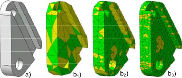
a) b1) b2) b3)
Fig. 1. Evolution of the mesh quality when increasing the
number of elements (from b1 to b3) during the meshing of
a CAD model (a).
N Q≥0.5 Q<0.5 Qworst Qmean
207 104 (50.24%) 103 (49.76%) 0.311 0.515 1100 876 (79.64%) 224 (20.36%) 0.334 0.582 4647 4372 (94.08%) 275 (5.92%) 0.402 0.623
Table 1. Mesh quality a posteriori estimation. Today, the meshing step is still a time-consuming iterative process where engineers spend a lot of time adjusting several control parameters (e.g. max devia-tion, target element size, number of elements, local refinements, etc.) before finding a good combination that generates an acceptable mesh with respect to the simulation requirements (e.g. without skinny ele-ments causing problems which can ruin a simula-tion). Often, the meshing is performed several times in loop since it is not possible to evaluate the mesh quality (e.g. aspect ratio, skew, taper, warp) before having generated the mesh. Actually, it is admitted that an element with an aspect ratio smaller than 0.5 can be considered as a “bad” element with respect to
the accuracy of the final simulation results [2]. Fig-ure 1 shows three meshes (fig. 1.b1 to 1.b3) generated
from the same CAD model (fig. 1.a) but using differ-ent elemdiffer-ent target sizes. It is clear that increasing the number of elements improves significantly the mesh quality thus resulting in less skinny and degenerated elements having an aspect ratio smaller than 0.5 (ta-ble 1). The worst and mean aspect ratios also get better. Mesh refinements can also be foreseen to adapt the size of the elements to the local configura-tions. Since this process is not fully automated, engi-neers still have to manually adjust the control param-eters to find a good balance between the quality of the mesh (to try to get more accurate simulation re-sults) and the speed of the resolution (strongly de-pending on the number of FE elements).
Actually, because there exists no bijective functions between the control parameters space and the result-ing mesh quality, the meshresult-ing process is necessarily iterative. This is mainly due to the fact that this map-ping between the mesh generator’s control parame-ters and the resulting mesh quality strongly relies on the characteristics of the shapes of the CAD model to be meshed. Moreover, since the effects of the control parameters overlap, it is even more difficult to cir-cumscribe the parameters’ individual effects and clearly identify simple rules to estimate the resulting quality.
This article addresses such a complex issue of under-standing the relationships and rules that drive the quality of a mesh generated from a CAD model, its shape characteristics and the mesh generator’s con-trol parameters. A framework is set up and aims at identifying those complex rules to be able to define a priori, i.e. before meshing the CAD model, which classes of mesh quality can be expected. It uses Ma-chine Learning Techniques (MLT) to discover those rules from a set of identified known configurations [17]. Each configuration is made of a CAD model, its associated shape characteristics, several meshes gen-erated from different values of the control parame-ters, and the classes of quality for each mesh. Shape characteristics refer to various shape descriptors such as a distance distribution function which characteriz-es the thickncharacteriz-ess of the part over the entire surface, or the ratio between the volume of the part and the vol-ume of its oriented bounding box which characterizes also how much the part is massive or empty. Each generated mesh is analysed and classified according to several mesh quality magnitudes such as the aspect ratio which measures the stretching of the elements.
Once the rules have been learnt, it is then possible to estimate a priori the classes of quality that can be expected for a part on which shape characteristics would have been extracted. Having such an a priori estimation, the designers do not spend too much time on the meshing issues since they can now better un-derstand the impact of some control parameters on the final mesh quality, and this without meshing the CAD model at first. Of course, once the parameters have been tuned, the meshing is performed one time without looping.
This framework has been implemented and validated on academic as well as industrial examples. It uses CATIA V5 for meshing the CAD model and evaluat-ing the mesh qualities of the learnt configurations, Matlab for extracting the CAD model’s shape char-acteristics and WEKA [8] to discover the rules and reply them on unknown configurations.
2. RELATED WORKS
The proposed framework uses MLT to identify rela-tionships between some characteristics of the CAD models to be meshed on one hand, and the character-istics of the generated meshes on the other hand.
2.1. Geometric models characterization
Reasoning on low-level geometric entities is not very easy for designers who are more interested in manip-ulating high-level description models and entities. For example, in the CAD context, feature-based ap-proaches have been set up to manipulate directly a set of faces through the feature concept [5][6]. To be more efficient and closer to the way people think, it is therefore important to focus on more advanced and structured approaches that use high-level quantities and models together with their associated semantics [1]. Thus, extracting shape characteristics from geo-metric models is an important field of research which finds numerous applications such as shape matching, shape retrieval, objects clustering and classification, design reuse, model comparison [4][7][9][10][11] [12][13][14]. Most of the time, the idea is to make the underlying algorithms work on high-level shape descriptors built on top of low-level geometric mod-els and data structures.
Many shape descriptors can be defined to character-ize geometric models. However, to charactercharacter-ize CAD models, it is important to underline that among the various shape descriptors, we have been focusing on those that could be most closely related to the mesh-ing issue. Effectively, durmesh-ing the learnmesh-ing phase, the
MLT will use those shape descriptors in place of the geometric models themselves. Therefore, having too few descriptors or not meaningful descriptors may generate invalid rules, whereas with too many de-scriptors the rules identification process can become more complex. Thus, a good balance has to be found with the selection of the most important ones which should also not overlap.
As demonstrated in [16], the so-called distance dis-tribution, inspired from the work of Osada et al. on the D2 shape distribution descriptor [15], is a good mean to characterize the evolution of the thickness of an object. Osada et al. use the distance distribution to characterize the overall shape of the object and dis-criminate objects with different gross shapes. It is computed by measuring the distance between points sampled over the surface. As developed in section 4.1, the D2 shape distribution descriptor has been adapted to our needs. It takes into account weighted distances between triangles instead of points. Other shape descriptors are also extracted from the CAD models: dimension of the Oriented-Bounding Box (OBB), volume of the object and volume of the OBB, ratio between those two volumes, overall area of the object (see section 4.1).
Considering the FE meshes, we have been focusing on classical descriptors even if there exists a huge amount of descriptors for estimating the quality of meshes [3]. Among them we focus on the aspect ratio as well as on the ratio high-width (see section 4.2).
2.2. MLT and uses in design
Machine learning is a branch of artificial intelligence which addresses the construction and study of sys-tems that can learn from data [17]. MLT are widely used in design activities [18] throughout the product lifecycle to address optimization problems [19], deci-sion making problems [20][21], shapes recognition [22], item recognition and extraction for reuse, recognition from point cloud and reverse engineering [2]. Recently, MLT have also been used to find rules to defeature CAD models for simulation [23].
3. OVERALL APPROACH
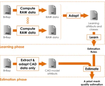
Our approach can be decomposed in several succes-sive steps forming an integrated and modular mesh quality estimation framework (fig. 2). Each step is further explained in sections 4 and 5. The approach being modular, each module can be replaced and/or optimized at a later development stage.
Fig. 2. Overview of the learning and estimation phases. During the learning phase (dot rectangle at the top of fig. 2), the different steps are organized as follows:
1) Compute RAW data from a set of B-Rep
mod-els stored in .step files. The intrinsic characteris-tics of the CAD models (thickness distributions, ratios between the volume of the OBB and vol-ume of the object, etc.) as well as the intrinsic characteristics of the newly generated FE tetra-hedral meshes (aspect ratios, ratios high-width, etc.) are extracted and aggregated in a set of .txt files forming the RAW data. This step is further developed in section 4.
2) Adapt RAW data to the needs of the
classifica-tion algorithms. It consists in transforming the RAW data in data which will be effectively used as inputs of the learning step. It is also during this step that a class of quality is assigned to each configuration. The adapted information are written in a .arff file which contains all the known configurations on which the learning will apply. This adaptation step is further developed in section 5.
3) Learn the rules from the known configurations
so that the quality classes can be estimated from the CAD model intrinsic characteristics.
Then, the estimation phase (dot rectangle at the bot-tom of fig. 2) can start for a CAD model which has not been used during the learning phase and for which the mesh quality is unknown:
4) Compute and adapt CAD data only with the
algorithms and criteria of steps 1) and 2), except that here the CAD model is not meshed and the mesh quality is not computed.
5) Estimate the class of quality while reapplying
the rules found in step 3) to the data computed in step 4). This corresponds to the a priori esti-mation step which is further explained in section 6. The class of quality is estimated without hav-ing to mesh the CAD model.
The implementation details are developed in section 6 which also gathers together the results.
4. COMPUTE INTRINSIC
CHARACTER-ISTICS OF GEOMETRIC MODELS
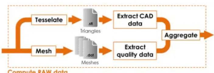
This section details the models, methods and tools that have been developed to compute the so-called RAW data from a B-Rep model and aggregate the results in a .txt files. Figure 3 zoom in the sub-steps of the “Compute RAW data” module first introduced on figure 2. As depicted, the idea is to separate the extraction of data from the CAD model from the ones related to the quality of FE meshes generated from the B-Rep model. To this aim, two pre-processing steps are run. On one hand, the B-Rep model is tessellated face by face and the resulting soup of triangles is stored in a .stl file. Shape scriptors are then computed. The adopted shape de-scriptors are further developed in section 4.1. On the other hand, the CAD model is meshed three times to generate different LOD (Levels Of Details) tetrahe-dral meshes stored in three .dat files. The .dat files are then analyzed to extract the corresponding mesh quality evaluations as explained in section 4.2. Both the extracted shape descriptors and mesh quality evaluations of the input B-Rep model are then aggre-gated in a unique .txt file whose entries form a so-called raw attributes vector (see section 4.3).
Fig. 3. Zoom in the “raw data computation” step.
4.1. CAD models’ shape descriptors
The shape descriptors extraction step works on a soup of triangles stored in a .stl file. The diagonal of the Oriented Bounding Box (OBB), its volume, the object volume, the ratio between the object volume and the OBB one, the object area, and the object
distance distribution are so many shape descriptors extracted from the .stl file.
Computing the minimal OBB of an object consists in finding a rectangular parallelepiped of minimal vol-ume enclosing a set of vertices distributed on the object surface. In our approach, those vertices are directly extracted from the .stl file. To get this mini-mal OBB, we use a famous and basic but efficient method which is the Principal Components Analysis (PCA). The PCA method computes the covariance matrix of the set of vertices. Then, the three axes of inertia are obtained by computing the eigenvectors of the covariance matrix, and the OBB can be easily defined in this local reference frame centred at the object barycentre. The three DBBi dimensions of the
bounding box are computed as the difference be-tween the maximum and the minimum coordinates of the object points on the three axes. These dimensions are ordered so that DBB1 ≥ DBB2 ≥ DBB3. The diagonal
of the OBB as well as its volume can be easily com-puted as follows:
diag ∑ D (1)
V D D D (2)
The calculation of the object area is straightforward and can be obtained by summing up the area of each triangle forming the object outer skin. Being Tk an
oriented triangle defined by its three ordered vertices
Pk, Pk+1 and Pk+2, the overall object area can be com-puted as follows:
Area ∑ Area T (3)
with Area T ^ . ⁄ (4) 2
Similarly, the object volume V is obtained by summing up the signed volumes of the oriented tet-rahedra whose bases are the oriented triangles Tk
forming the object outer skin, and with the object barycenter as a common summit [16].
However, it would not be meaningful to build classi-fication criteria on top of shape descriptors that would use absolute basic quantities like area or vol-ume. Hence, the computation of the minimal OBB is used as a mean to evaluate how much the object is filled or rather empty with respect to its bounding box. As a consequence, the following ratio is introduced as a shape descriptor:
Finally, one of the main descriptors used in our work is the so-called distance distribution, inspired from the work of Osada et al. on the D2 shape distribution descriptor [15]. It helps understanding the evolution of the object thickness by summing up the occur-rences of characteristic distances over the entire ob-ject. It is computed from the soup of triangles stored in the .stl file. To this aim, pairs of triangles facing each other have to be identified using the following functions: 1 if π 0 and π 0 and π 0 0 otherwise (6) with π det , , (7)
wherein , and are the three summits of the triangle T , and the normal to the triangle comput-ed with :
^ ⁄‖ ^ ‖ (8)
In other words, when 1 the projection of in the plane defined by T lies inside the triangle. Therefore, for each couple of triangle T and T , the following criterion is used to identify triangles facing each other:
. 1 (9)
with and the barycenters of respectively T and T . When two triangles are considered as facing each other, the following distance is tagged as being a characteristic distance and the corresponding value d is put in a list of distances L :
(10)
The list of N characteristic distances is then normal-ized according to the diagonal of the OBB to get a normalized list L :
L with ∀k ∈ 1. . N , L k ∈ 0,1 (11)
Being O L, , the function that computes the number of elements of a list L which occur in the range , , and N the number of slots used to split the interval [0, 1], the final normalized distance distribution list L is filled as follows:
∀k ∈ 1, N , L k O L , , /N (12)
with k 1 /N
Figure 4 shows the result of this algorithm on a half-carter with N 50 slots. One can notice that 33% of
the characteristic distances refer to areas character-ized by a thickness that is in between 2% and 4% of the OBB diagonal. It reveals that the half-carter has a main thickness. Distance (%) Tessellation Thickness (%) 33% OBB 4% 2%
Fig. 4. Normalized distance distribution on a half-carter.
4.2. Mesh quality descriptors
As introduced in section 3, for each B-Rep model, three FE tetrahedral meshes are generated (fig. 3) and analysed according to several descriptors:
-
The aspect ratio of each element, the minimal,maximal and mean values of those aspect ratio as well as the percentage of good elements, i.e. elements having an aspect ratio Q 0.3 in the present case. The aspect ratio of a tetrahedron is computed according to the method presented in [2];
-
The ratio high-width Q max ℓ / min ℓ of each element, being ℓ , ∈ 1. .6 the lengths of the six edges of a tetrahedron.Clearly, this set of quality descriptors could be ex-tended in the future.
4.3. Raw vector data
All the data extracted from the B-Rep models and corresponding tessellated and FE models can be con-sidered as RAW data that should be adapted in a later stage.
For example, the distance distribution is too complex to be inserted as it in a Machine Learning algorithm. Thus, the data need to be filtered and adapted so as to get less independent values but still representing accurately the distance distribution.
5. RAW DATA ADAPTATION AND PART
CLASSIFICATION
Before starting the learning process, the raw data have to be adapted and the parts classified.
Distance (%) Thickness (%) p1 p2 x2 x1
Fig. 5. Extraction of key points on a normalized distance
distribution.
As explained in section 4.3, the normalized distance distribution needs to be adapted to avoid inserting several tens of distance values into the learning algo-rithm. Among the various descriptors that have been tested, some help understanding the shapes of the parts and thus better evaluate the potential meshing difficulties. Those descriptors are based on the identi-fication of the two couples x , p and x , p . p is the greatest percentage of the normalized distance distribution histogram and x the corresponding rela-tive distance. p is the second greatest percentage and x the corresponding relative distance. Based on those values, four descriptors are computed:
- DA N N⁄ ∈ 0, 1 , being N the number of characteristic distances displayed in the histo-gram (N 15 on the histogram of fig. 5) and N the number of slots (N 50 on the histogram of fig. 5). The more this descriptor is important, the more the part has an important number of char-acteristic distances, the more the shapes are complex (fillets, chamfers, …) and the more the part will be difficult to mesh;
- DA x x ∈ 1, 1 . The more |DA | is
close to 1, the more the two relative distances x and x are distinct which means which may lead to meshing problems. If DA 0, it means that the greatest relative distance is smaller than the
second one which can generate more meshing issues than if this descriptor is positive;
- DA p p⁄ ∈ 0, 1 . If this descriptor is close to 1, it means that the two main relative distanc-es coexist in the same proportions. Thus, if at the same time |DA | is important, this may also lead to meshing issues;
- DA min x , x . The more this descriptor is close to 0, the more it will be difficult to mesh this part thus characterized by a small character-istic distance.
At the end, the normalized distance distribution is not used as it in the learning phase. It is adapted and transformed into four DA meaningful descriptors. Now that all the descriptors have been extracted and adapted, it is important to focus on the classification of the parts. Effectively, since the idea is to use a classification algorithm based on MLT, it is neces-sary to provide a class for each configuration (i.e. part in the present case) that will be analysed. In this work, the classification is directly based on the quali-ty of the three FE meshes generated for each part. For the i part, three FE meshes ,, j ∈ 1. .3 are generated and analyzed. It is supposed that there are less elements in , than in , , and there are less elements in , than in , . In the proposed im-plementation, , has about 100 tetrahedra, , about 1000 and , about 5000. For each mesh, the percentage of good element PQ, is extracted, i.e. the percentage of elements having an aspect ratio greater than 0.3. Based on this, three classifiers are evaluated as follows:
If PQ, 80% then CL, 1,
Else If PQ, ∈ 60%, 80% then CL, 2
Else If PQ, 60% then CL, 3.
Based on top of those classifiers, four classes are distinguished:
If CL, CL, OR CL, CL, then The i part is tagged as unlogical since there
is no reason why to have a mesh quality de-creasing when the number of elements increas-es;
Else If CL, 1 then
The part is classed as “A” meaning that its
meshing is not difficult since we obtain good results with few elements;
Else If CL, 1 AND CL, 1 then The part is classed as “B” meaning that its
meshing is more difficult than in the case of a class “A” part.
Else If CL, 1 and CL, 1 and CL, 1 then
The part is classed as “C” meaning that its
meshing is more difficult than in the case of a class “B” part.
Else The part is classed as “D”.
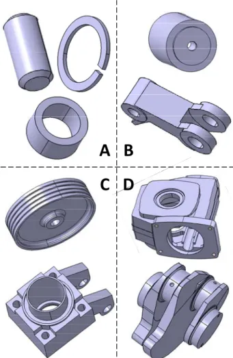
In the proposed implementation, the number of clas-ses has been reduced to decrease the complexity of the learning phase. This is also due to the fact that with few classes, we need to have fewer parts as in-puts of the learning algorithm. One can also notice that this classification has no upper limit in the sense that the last class may contain parts difficultly mesh-able as well as parts very very very difficulty mesha-ble. Figure 6 shows examples of parts classified ac-cording to the four above described classes.
A B
C D
Fig. 6. Examples of parts classified in four classes
according to meshing issues.
6. RESULTS & DISCUSSION
The proposed approach uses CATIA V5 and VBA macros to tessellate the parts and export the triangu-lation in a .stl file, Matlab to extract all the shape descriptors from the soups of triangles and adapt them to WEKA that is used in the last stage for learn-ing and testlearn-ing the rules.
The experimentation has been performed on a set of industrial and academic parts including 28 parts of each class A, B, C and D. Thus, the initial database is made of 112 instances. For these parts, all the previ-ously introduced shape descriptors have been ex-tracted and adapted (sections 4 and 5). In addition, the number of features (holes, ribs, etc.) is also ex-tracted. To better evaluate the influence of the vari-ous attributes during the experimentations, several groups of attributes have been defined:
G bodies, shapes, pads, pockets, holes, shafts, ribs, mirrors, chamfers, slots,
constradedgefillets, grooves
DA , DA and DA , DA
diag , V , V , Area
The group of attributes are then combined in 5 exper-imental lists as follows:
∀k ∈ 1. .5 , E ⋃ G (13) For each experimental list, three classification algo-rithms are tested: Naïve Bayes, Multilayer Percep-tron and J48 Tree [17]. For each algorithm, the eval-uation is performed in three different ways: using the Training Set (TS) so that all the instances are used to learn as well as to test, using Cross-Validation (CV) with decompositions in sets of 10%, and using Per-centage Split (PS) to learn on 66% and test on 34%.
Test E1 E2 E3 E4 E5 Naïve Bayes TS 41.1 46.4 47.3 63.4 67.9 CV 34.8 40.2 40.2 52.7 56.3 PS 36.8 42.1 44.7 60.5 55.3 Multilayer Perceptron TS 67.8 77.7 81.3 83.0 86.6 CV 50.0 52.7 55.3 50.9 53.6 PS 47.4 52.6 50.0 47.4 52.6 J48 Tree TS 63.4 73.2 84.8 86.6 88.4 CV 47.3 53.6 46.4 53.6 56.3 PS 47.3 47.4 47.4 55.3 55.3
Table 2. Percentage of correctly classified instances
de-pending on the algorithm (Naïve Bayes, Multilayer Per-ceptron, J48 Tree), the type of test (FS, CV, PS) and the type of attributes (E1 to E5).
The results of the various experimentations are gath-ered together in Table 2. Generally speaking, one can notice that the use of the Training Set (TS) gives better results than the use of the Cross-Validation (CV) which gives better results than the Percentage Split (PS). This is due to the fact that for TS, all the instances are used to learn and to test. Therefore, the test is performed on instances on which the system has been trained. One can also notice that the per-centage of well-classified instances is getting better when the number of attributes increases. This cannot become a general rule. However, it clearly demon-strates that the selection of the attributes has a strong impact on the classification results. More experimen-tations Ek have to be performed to clearly identify a
restricted set of attributes.
Among the various experimentations, one can zoom on E5 using the J48 tree with the CV testing option.
In this case, we get 56.3% of well classified instanc-es. The confusion matrix is as follows:
C 17 9 2 0 6 17 4 1 0 6 13 9 1 5 6 16 (14) The lines of the matrix gather together the infor-mation relative to the classes. Line 1 corresponds to class A and so on for the other lines. The rows corre-spond to classes in which the tested instances have been put when using the classification rules that have been learnt. For example, 13 instances of class C have been well classified as class C instances during the testing phase. However, 5 instances of class D have been classed as class B instances. Ideally, this matrix should be diagonal. In our case, having num-bers in the upper part of the matrix is not a real prob-lem since the badly classified instances would be somehow over-classed. Effectively, over-classing an instance will generate over-quality which is accepta-ble. However, having numbers under the diagonal may generate badly meshed parts.
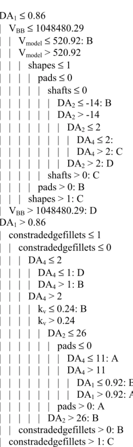
The output of the J48 algorithm is a decision tree as depicted on figure 7. This tree has been obtained in less than 0.1s on an Intel Core Duo 2.66GHz. Using this tree, unknown examples can be classified easily in any environment and there is no need to use WE-KA afterwards. For example, if a part is classed B, it means that about 1000 elements are enough to have a good quality of the mesh. Said differently, if classi-fied B, 100 elements won’t be enough to have a good quality. Using such an approach, the mesh quality can be estimated a priori, i.e. without having to mesh
the part. This is also verified by the fact that no at-tributes used in the tree refer to the meshes.
DA1≤ 0.86 | VBB≤ 1048480.29 | | Vmodel≤ 520.92: B | | Vmodel > 520.92 | | | shapes ≤ 1 | | | | pads ≤ 0 | | | | | shafts ≤ 0 | | | | | | DA2≤ -14: B | | | | | | DA2 > -14 | | | | | | | DA2≤ 2 | | | | | | | | DA4≤ 2: | | | | | | | | DA4 > 2: C | | | | | | | DA2 > 2: D | | | | | shafts > 0: C | | | | pads > 0: B | | | shapes > 1: C | VBB > 1048480.29: D DA1 > 0.86 | constradedgefillets ≤ 1 | | constradedgefillets ≤ 0 | | | DA4≤ 2 | | | | DA4≤ 1: D | | | | DA4 > 1: B | | | DA4 > 2 | | | | kv≤ 0.24: B | | | | kv > 0.24 | | | | | DA2≤ 26 | | | | | | pads ≤ 0 | | | | | | | DA4≤ 11: A | | | | | | | DA4 > 11 | | | | | | | | DA1≤ 0.92: B | | | | | | | | DA1 > 0.92: A | | | | | | pads > 0: A | | | | | DA2 > 26: B | | constradedgefillets > 0: B | constradedgefillets > 1: C
Fig. 7. Decision tree with 19 leaves obtained using the J48
algorithm on E5 and Cross-Validation for testing.
Finally, it is important to understand that the quality of the learning step strongly relies on the number of instances, the attributes that are selected, the adopted classification algorithm and its parameters. Now that the overall framework is set up, next steps include a deeper analysis of those aspects. But clearly, the J48 tree algorithm already gives interesting results. The rules are simple and can easily be implemented in any CAD environment to help designers better esti-mating the quality of their future meshes.
7. CONCLUSION
In this paper, a new framework has been set up to help engineers understanding FE meshing issues a priori, i.e. before meshing the parts. This is a first step towards the definition of an a priori mesh quality estimator. The process starts from a set of parts on which we can extract characteristics relative to their shapes, as well as characteristics relative to several generated FE meshes. Based on those extracted quan-tities/attributes, the parts can be classified. From this classification, we use MLT to find interesting classi-fication rules so that those rules can be reapply on unknown data for which the class will be estimated a priori. In the present implementation, four classes are used to classify the parts according to the meshing complexity while keeping in mind the following rule: part difficultly meshable will generate bad quality meshes if the number of Finite Elements is not great enough.
The approach is modular and the different modules can be optimized. It gives interesting and promising results. We now have to concentrate on the way the percentage of good classification can be optimized and thus increased. Three directions are envisaged. The first consists in reworking on the attributes used to characterise the parts and the meshes. The second concerns the adaptation phase where RAW data are transformed in data adapted for the leaning phase. The third is relative to the adopted MLT algorithms and associated control parameters. In this last case, the use of numeric classifiers will help us finding rules to estimate a priori and numerically the mean aspect ratio of the future not yet generated meshes. In the future, the training set will also be enlarged to host additional classified parts.
The proposed framework can also be foreseen for other applications like the a priori estimation of stress errors.
REFERENCES
[1] Aim@Shape, (2004), European NoE, Key Action 2.3.1.7 on Semantic-based Knowledge Systems, VI Framework, URL: http://www.aimatshape.net. [2] Bern, M. and Plassman, P., (2000), Mesh generation,
in Sack J.-R. and Urrutia J. (Eds), Handbook of Com-putational Geometry, Elsevier Science Publishers, B.
V. North-Holland, Amsterdam, The Netherlands, pp. 291-332.
[3] Frey, P-J., George, P-L., (2008), Mesh generation: Application to finite elements, second edition, Wiley, London, 848 pages.
[4] Iyer, N., Jayanti, S., Lou, K., Kalyanaraman, Y. and Ramani, K., (2005), Three-dimensional shape searching: state-of-the-art review and future trends,
Computer-Aided Design, Vol. 37, No. 5, pp. 509-530.
[5] Pernot, J-P., Falcidieno, B., Giannini, F., Léon, J-C.,
Incorporating free-form features in aesthetic and en-gineering product design: State-of-the-art report,
Computers in Industry, vol. 59(6), pp. 626-637, 2008. [6] Shah, J. J. and Mäntylä, M., ( 1995), Parametric and
Feature-based CAD/CAM, John Wiley & Sons, Inc.,
New York.
[7] Tangelder, J. and Veltkamp, R., (2008), A survey of
content based 3D shape retrieval methods,
Multime-dia Tools and Applications, Vol. 39, No. 3, pp. 441-471.
[8] http://www.cs.waikato.ac.nz/ml/weka/
[9] Li, M., Zhang, Y.F. and Fuh, J.Y.H., (2010),
Retriev-ing reusable 3D CAD models usRetriev-ing knowledge-driven dependency graph partitioning,
Computer-Aided Design and Applications, Vol. 7, No. 3, pp.417-430.
[10] Demirci, M.F., van Leuken, R.H. and Veltkamp, R.C., (2008), Indexing through Laplacian spectra,
Computer Vision and Image Understanding, Vol. 110, No. 3, pp. 312-325.
[11] Zhu, K., San Wong, Y., Tong Loh, H. and Feng Lu, W., (2012), 3D CAD model retrieval with perturbed Laplacian spectra, Computers in Industry, Vol. 63,
No. 1, pp. 1-11.
[12] Brière-Côté, A., Rivest, L. and Maranzana, R., (2012), Comparing 3D CAD Models: Uses, Methods, Tools and Perspectives, Computer-Aided Design and
Applications, Vol. 9, No. 6, pp. 771-794.
[13] Bai, J., Gao, S., Tang, W., Liu, Y. and Guo, S., (2010), Design reuse oriented partial retrieval of CAD models, Computer-Aided Design, Vol. 42, No.
12, pp. 1069-1084.
[14] Jayanti, S., Kalyanaraman, Y. and Ramani, K., (2009) Shape-based clustering for 3D CAD objects: A comparative study of effectiveness,
Computer-Aided Design, Vol. 41, No. 12., pp. 999-1007. [15] Osada, R., Funkhouser, T., Chazelle, B. and Dobkin,
D., (2002), Shape distributions, ACM Transactions
on Graphics, Vol. 21, No. 4, pp. 807-832.
[16] Pernot, J.-P. , Giannini, F. and Petton, C., (2012),
Categorization of CAD models based on thin part identification, in proceedings of TMCE’12,
Karls-ruhe, Germany.
[17] Mitchell, T., (1997), Machine Learning, McGraw Hill.
[18] Renner, G., (2004), Genetic algorithms in computer
aided design, Computer-Aided Design and
Applica-tions, Vol. 1, No. 1-4, pp. 691-700.
[19] Shi, B.-Q., Liang, J., Liu, Q., (2011), Adaptive
sim-plification of point cloud using k-means clustering,
Computer-Aided Design, Vol. 43, No. 8, pp. 910-922.
[20] Lee, S.H., (2005), A CAD-CAE integration approach
using feature-based resolution and multi-abstraction modelling techniques, Computer-Aided
Design, Vol. 37, No. 9, pp. 941-955.
[21] Sun, R., Gao, S., Zhao, W., (2010), An approach to
B-Rep model simplification based on region suppres-sion, Computers & Graphics, Vol. 34, No. 5, pp.
556-564.
[22] Jayanti, S., Kalyanaraman, Y., Ramani, K., (2009),
Shape-based clustering for 3D CAD objects: A com-parative study of effectiveness, Computer-Aided
De-sign, Vol. 41, No. 12, pp. 999-1007.
[23] Gujarathi, G.P., Ma, Y.-S., (2011), Parametric
CAD/CAE integration using a common data model,
Jou. of Manufacturing Systems, Vol. 30, No. 3, pp. 118-132.