Université de Montréal
Advances in Deep Learning Methods for Speech Recognition and Understanding
par Dmitriy Serdyuk
Département d’informatique et de recherche opérationnelle Faculté des arts et des sciences
Thèse présentée à la Faculté des arts et des sciences en vue de l’obtention du grade de Philosophiæ Doctor (Ph.D.)
en informatique
octobre, 2020
Résumé
Ce travail expose plusieurs études dans les domaines de la reconnaissance de la parole et compréhension du langage parlé. La compréhension sémantique du lan-gage parlé est un sous-domaine important de l’intelligence artificielle. Le traite-ment de la parole intéresse depuis longtemps les chercheurs, puisque la parole est une des charactéristiques qui definit l’être humain. Avec le développement du réseau neuronal artificiel, le domaine a connu une évolution rapide à la fois en terme de précision et de perception humaine. Une autre étape importante a été franchie avec le développement d’approches bout en bout. De telles ap-proches permettent une coadaptation de toutes les parties du modèle, ce qui aug-mente ainsi les performances, et ce qui simplifie la procédure d’entrainement. Les modèles de bout en bout sont devenus réalisables avec la quantité croissante de données disponibles, de ressources informatiques et, surtout, avec de nombreux développements architecturaux innovateurs. Néanmoins, les approches tradition-nelles (qui ne sont pas bout en bout) sont toujours pertinentes pour le traitement de la parole en raison des données difficiles dans les environnements bruyants, de la parole avec un accent et de la grande variété de dialectes.
Dans le premier travail, nous explorons la reconnaissance de la parole hy-bride dans des environnements bruyants. Nous proposons de traiter la reconnais-sance de la parole, qui fonctionne dans un nouvel environnement composé de différents bruits inconnus, comme une tâche d’adaptation de domaine. Pour cela, nous utilisons la nouvelle technique à l’époque de l’adaptation du domaine antag-oniste. En résumé, ces travaux antérieurs proposaient de former des caractéris-tiques de manière à ce qu’elles soient distinctives pour la tâche principale, mais non-distinctive pour la tâche secondaire. Cette tâche secondaire est conçue pour être la tâche de reconnaissance de domaine. Ainsi, les fonctionnalités entraînées sont invariantes vis-à-vis du domaine considéré. Dans notre travail, nous adoptons cette technique et la modifions pour la tâche de reconnaissance de la parole dans un environnement bruyant.
Dans le second travail, nous développons une méthode générale pour la régu-larisation des réseaux génératif récurrents. Il est connu que les réseaux récurrents ont souvent des difficultés à rester sur le même chemin, lors de la production de sorties longues. Bien qu’il soit possible d’utiliser des réseaux bidirectionnels pour une meilleure traitement de séquences pour l’apprentissage des charactéris-tiques, qui n’est pas applicable au cas génératif. Nous avons développé un moyen d’améliorer la cohérence de la production de longues séquences avec des réseaux récurrents. Nous proposons un moyen de construire un modèle similaire à un
réseau bidirectionnel. L’idée centrale est d’utiliser une perte L2 entre les réseaux récurrents génératifs vers l’avant et vers l’arrière. Nous fournissons une évaluation expérimentale sur une multitude de tâches et d’ensembles de données, y compris la reconnaissance vocale, le sous-titrage d’images et la modélisation du langage.
Dans le troisième article, nous étudions la possibilité de développer un iden-tificateur d’intention de bout en bout pour la compréhension du langage parlé. La compréhension sémantique du langage parlé est une étape importante vers le développement d’une intelligence artificielle de type humain. Nous avons vu que les approches de bout en bout montrent des performances élevées sur les tâches, y compris la traduction automatique et la reconnaissance de la parole. Nous nous inspirons des travaux antérieurs pour développer un système de bout en bout pour la reconnaissance de l’intention.
Mots clés: apprentissage profond, apprentissage automatique, reconnaissance de la parole, réseaux de neurones, adaptation de domaine, reconnaissance de la pa-role bruyante, apprentissage antogoniste, réseaux de neurones récurrents, généra-tion de séquences, compréhension du langage vocal, apprentissage de bout en bout.
Abstract
This work presents several studies in the areas of speech recognition and under-standing. The semantic speech understanding is an important sub-domain of the broader field of artificial intelligence. Speech processing has had interest from the researchers for long time because language is one of the defining characteristics of a human being. With the development of neural networks, the domain has seen rapid progress both in terms of accuracy and human perception. Another impor-tant milestone was achieved with the development of end-to-end approaches. Such approaches allow co-adaptation of all the parts of the model thus increasing the performance, as well as simplifying the training procedure. End-to-end models became feasible with the increasing amount of available data, computational re-sources, and most importantly with many novel architectural developments. Nev-ertheless, traditional, non end-to-end, approaches are still relevant for speech pro-cessing due to challenging data in noisy environments, accented speech, and high variety of dialects.
In the first work, we explore the hybrid speech recognition in noisy environ-ments. We propose to treat the recognition in the unseen noise condition as the domain adaptation task. For this, we use the novel at the time technique of the adversarial domain adaptation. In the nutshell, this prior work proposed to train features in such a way that they are discriminative for the primary task, but non-discriminative for the secondary task. This secondary task is constructed to be the domain recognition task. Thus, the features trained are invariant towards the domain at hand. In our work, we adopt this technique and modify it for the task of noisy speech recognition.
In the second work, we develop a general method for regularizing the gener-ative recurrent networks. It is known that the recurrent networks frequently have difficulties staying on same track when generating long outputs. While it is pos-sible to use bi-directional networks for better sequence aggregation for feature learning, it is not applicable for the generative case. We developed a way improve the consistency of generating long sequences with recurrent networks. We pro-pose a way to construct a model similar to bi-directional network. The key insight is to use a soft L2 loss between the forward and the backward generative recur-rent networks. We provide experimental evaluation on a multitude of tasks and datasets, including speech recognition, image captioning, and language modeling.
In the third paper, we investigate the possibility of developing an end-to-end intent recognizer for spoken language understanding. The semantic spoken lan-guage understanding is an important step towards developing a human-like arti-ficial intelligence. We have seen that the end-to-end approaches show high per-formance on the tasks including machine translation and speech recognition. We draw the inspiration from the prior works to develop an end-to-end system for intent recognition.
Key words: deep learning, machine learning, speech recognition, neural net-works, domain adaptation, noisy speech recognition, adversarial learning, recur-rent neural networks, sequence generation, spoken language understanding, end-to-end learning.
Contents
List of Figures 5
List of Tables 7
1 Introduction 9
1.1 Presented Papers . . . 10
1.1.1 Invariant Representations for Noisy Speech Recognition . 10 1.1.2 Twin Networks: Matching the Future for Sequence Gen-eration . . . 12
1.1.3 Towards End-to-end Spoken Language Understanding . . 13
1.2 Artificial Intelligence . . . 14
1.3 The Role of Speech Processing in the Development of Artificial Intelligence . . . 16
1.4 Audio and Speech Applications . . . 17
2 Background 19 2.1 Machine Learning . . . 19
2.1.1 General Setup . . . 19
2.1.2 Bias-Variance trade-off: Underfitting and Overfitting . . . 21
2.2 Deep Learning . . . 23
2.2.1 Optimization . . . 25
2.2.2 Regularization . . . 28
2.2.3 Autoregressive Models . . . 28
2.2.4 Recurrent Neural Networks . . . 31
2.2.5 Long Short-Term Memory recurrent networks . . . 31
2.2.6 Sequence Generation with Recurrent Neural Networks . . 32
2.3 Automatic Speech Recognition . . . 35
2.3.2 End-to-end Systems . . . 37
2.4 End-to-end Large Vocabulary Speech Recognition . . . 39
2.4.1 Introduction . . . 39
2.4.2 Model for Large Vocabulary Speech Recognition . . . 39
2.4.3 Integration with a Language Model . . . 40
3 Adversarial Training of Invariant Features for Speech Recognition 43 3.1 Context . . . 43
3.2 Introduction . . . 44
3.3 Background . . . 45
3.4 Related Work . . . 47
3.5 Invariant Representations for Speech Recognition . . . 49
3.6 Experiments . . . 50
3.7 Conclusion . . . 52
4 Twin Networks: Matching the Future for Sequence Generation 53 4.1 Context . . . 53
4.2 Twin Networks: Introduction . . . 58
4.3 Model . . . 60
4.4 Related Work . . . 62
4.5 Experimental Setup and Results . . . 63
4.6 Discussion . . . 68
5 Towards End-to-end Spoken Language Understanding 71 5.1 Context . . . 71
5.2 Introduction . . . 73
5.3 Standard ASR and NLU systems . . . 75
5.4 End-to-end Spoken Language Understanding . . . 77
5.5 Experiments . . . 78
5.6 Results and discussion . . . 80
List of Figures
2.1 Overfitting example. . . 22
2.2 Two layer neural network. . . 26
2.3 Decision boundaries. . . 27
2.4 Bidirectional RNN stack. . . 33
2.5 Attention mechanism. . . 34
2.6 Weighted finite state transducer. . . 37
2.7 Pooling in bidirectional RNN. . . 40
3.1 Domain adaptaion neural network illustraion. . . 50
3.2 Word error rates for adaptation models. . . 50
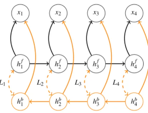
4.1 Twin Network model conceptual illustration. . . 60
4.2 Analysis for speech recognition experiments with Twin Networks 66 4.3 Analysis of the L2 loss for Twin Networks. . . 68
5.1 Traditional spoken language understanding system. . . 74
5.2 Automatic speech recognition system. . . 75
5.3 Natural language understanding. . . 76
5.4 End-to-end spoken language understanding system. . . 77
List of Tables
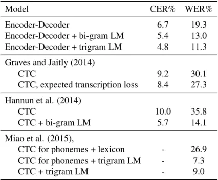
2.1 Results for attention-based large vocabulary speech recognition. . 42
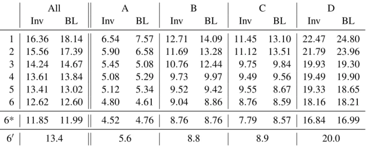
3.1 Performance of domain adaptation system on Aurora-4. . . 51
4.1 Analysis of speech recognition experiments with Twin Networks . 64 4.2 Results of experiments for image captioning with TwinNet. . . 67
4.3 Results for binarized sequential MNIST. . . 69
4.4 Results for WikiText-2 and Penn TreeBank . . . 70
5.1 Results for domain classification. . . 80
Chapter 1
Introduction
This general theme of this document is the development of methods to recog-nize spoken signal and understanding the human speech using novel deep learning architectures. The ability to exchange information via sounds is an essential as-pect of human intelligence. Therefore, I believe that studying the mechanisms of spoken interaction is one of the most important building bricks for hypothetical general artificial intelligence as well a useful tool for many practical applications. Despite the fact that there was several decades of research progress in the areas of speech processing and machine learning, there are many unresolved questions. One of the most important milestones in the field was the development and adop-tion of deep learning. It allowed to significantly increase the quality of speech processing, including speech recognition and synthesis. Nevertheless, there is still space for improvement.
First, many speech recognition systems are not enough robust to noisy envi-ronments, accented speech, and variable recording hardware. It is known that speech recognition rapidly degrades in challenging environments. Such envi-ronments are crowded places, where many persons talk simultaneously; airports, where some fragments of speech are completely obstructed by background noise; roads and factories, where background noise constantly interferes with the speech. The second shortcoming originates from an architecture which is widely used in deep learning systems dealing with sequentual inputs or outputs. This is the case for speech processing, where a single utterance can be as long as several thousands frames long. Dealing with the information flow through the long se-quences is generally hard. Despite the numerous attempts to tackle the issue, long sequences generated with state of the art models at the time were unable to keep the consistency throughout the whole length.
The third issue concerns understanding the spoken language. A usual way to perform such a task is to have a pipeline of a recognizer followed by a natural language processing component. Meanwhile, it has been shown that end-to-end approach is superior in many cases because it allows to optimize all the compo-nents in tandem and allows them to co-adapt. Therefore, building an end-to-end systems for understanding spoken language is an important task.
Attempting to solve three issues defined above, this work presents three pa-pers:
1. Invariant Representations for Noisy Speech Recognition, published at Neu-ral Information Processing Systems 2016 workshop on End-to-end Learn-ing for Speech and Audio ProcessLearn-ing by Dmitriy Serdyuk, Kartik Audhkhasi, Philémon Brakel, Bhuvana Ramabhadran, Samuel Thomas, Yoshua Bengio (see Chapter 3);
2. Twin Networks: Matching the Future for Sequence Generation, published at International Conference on Learning Representations 2018 by Dmitriy Serdyuk, Nan Rosemary Ke, Alessandro Sordoni, Adam Trischler, Chris Pal, Yoshua Bengio (see Chapter 4);
3. Towards End-to-end Spoken Language Understanding, published at Inter-national Conference on Acoustics, Speech and Signal Processing by Dmitriy Serdyuk, Yongqiang Wang, Christian Fuegen, Anuj Kumar, Baiyang Liu, Yoshua Bengio (see Chapter 5).
1.1
Presented Papers
The subsections below give a brief reference for each paper as well as the statement of contribution.
1.1.1
Invariant Representations for Noisy Speech Recognition
Modern speech recognition systems are very powerful when run with clean and predictable signal. Unfortunately, this is not the case when the environment is noisy. The quality rapidly degrades with the background noise. This effect is especially pronounced when the speech recognition system encounters an envi-ronmental condition is was not trained for.
A recent work [42] proposed to use adversarial training methods to perform model adaptation. In the nutshell, they train the model to perform the task at hand while at the same time injecting a signal in the middle which dictates not to distinguish domains. Hence, this is called adversarial training – the part of the model is optimized to perform badly an auxiliary task. The injected signal makes the model to learn features that are similar across different domains but are suited well for the main task.
In our publication Invariant Representation for Noisy Speech Recognition, my co-authors and me developed a method based on [42]. The method is using an adversarial adaptation training to improve speech recognition in noisy environ-ments. Reformulating the task as domain adaptation helped us to improve the baseline system and to better understand the extents of applicability of the adver-sarial adaptation technique.
We performed numerous rigorous experiments testing a hybrid MLP-HMM system using a well-benchmarked Aurora-4 noisy speech corpus. In our exper-iments we tested the performance of the system when trained on a small subset of noise conditions and tested on a different subset of conditions. We tested the simulated noise, as well the genuine one. Furthermore, we tested the adaptation to different recording conditions (utterances captured with a different microphone).
Statement of Contribution
The author of this thesis was was the leading author for this paper. My contri-butions of the first author to this work are:
1. He found the primary idea to use the adversarial domain adaptation to learn invariant representations;
2. He proposed model for learning invariant representations;
3. He proposed the set of experiments to test the performance of the model; 4. He conducted the majority of the experiments.
The other authors provided me with invaluable help with the dataset preparation, consultation, brain storming, and help with the experiments.
1.1.2
Twin Networks: Matching the Future for Sequence
Gen-eration
Generative recurrent networks are notoriously hard to train. One of the prob-lems is that the generated text samples are not consistent throughout long se-quences. This can be observed with unconditional generation, when a generative model is trained to produce text given previous piece of text. In such a scenario, recurrent generative networks tend to go off the rails when asked to generate suf-ficiently long texts. The conditional generative neural models are also affected by this problem, although to smaller extent.
This work considers a family of recurrent networks that have some hidden state. This includes simple Elman recurrent networks, recurrent networks com-posed of Long Short-Term Memory (LSTM) cells, or Gated Recurrent Unit (GRU) cells. The recurrent hidden state is connected to all the previous inputs through the previous hidden states. Furthermore, the hidden state is what is used to generate the following outputs. Therefore, in this work we hypothesized that the repre-sentation contained in the recurrent hidden state is the summarization of all the previous time-steps which is necessary for producing the following time-steps.
In this work, we developed a method to help a recurrent network to generate more consistent samples. Because of the nature of the factorization of the total probability of the output sequence, the generation has to be performed in a single direction. Although, bi-directional networks are well-suited for sequence repre-sentation learning, it is hard to use them for sequence generation. Therefore, the first motivation for this work is to develop a way to use bi-directional network for generation.
The second motivation comes from the fact that the hidden state summarizes all the previous states. Now, let us consider a network that generates the same sequence in the opposite direction. The hidden state of the backward-running network is the summarization of all the future states. It means that learning to predict the backward hidden state has to help to generate more consistent samples. Driven by these motivations we develop a method to regularize generative recurrent networks. In the nutshell, we train an extra recurrent network to generate the same sequence backwards. Then, the co-temporal states are tied together via an L2 loss. This loss is only used during the training. Then, during the testing, the backward-running network is discarded and the generation is performed as usual. This regularization method yielded consistent performance for a multitude of tasks and datasets. We performed the experiments with speech recognition, image captioning, language modelling, and pixel-by-pixel recurrent image generation
tasks.
Statement of Contribution
The author of this thesis was leading the research effort on the Twin Networks project. My contributions are:
1. Together with the second author he developed the idea of Twin Networks; 2. He conducted the experiments on speech recognition;
3. He conducted a half of the experiments on image captioning.
The shared first author contributed in the development of the twin networks, con-ducted several experiments in image captioning and language modeling. The third author conducted the majority of the experiments for language modelling and the image generation. The other authors contributed in the discussion, brainstorming and planning the research effort.
1.1.3
Towards End-to-end Spoken Language Understanding
Spoken language understanding is a task that is familiar to most people through the digital assistants. The user utters a command, such as “What is the weather today?”, then the assistant is expected to respond to the command, for example looking up and reporting the weather. Modern spoken language understanding systems work in several stages. Usually, in order to understand the user’s query, the assistant transcribes it first into a text input, then feeds the text into the natural language understanding model. In other words, spoken language understanding requires training a speech recognizer as well as a natural language understanding model.
With the development of end-to-end learning systems, new breakthroughs were achieved in a diverse set of machine learning tasks. These tasks include machine translation, speech recognition, image captioning, and speech synthesis. The end-to-end paradigm allows the components of the system to co-adapt. Op-timizing all the components for the required task loss (or its surrogate) helps to achieve state of the art performance in many cases.
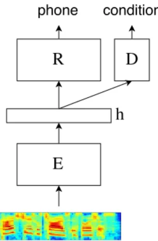
In this work we investigate the possibility to train in conjunction the recognizer and the language understanding parts. To make the first step toward end-to-end learning, we train the intent recognizer without an intermediate text transcription.
We employ the multitude of the tricks from the literature on end-to-end speech recognition. Our experimental results show a great potential in this line of re-search. Although, we do not reach the state of the art for this task, we show similar performance using drastically less computation. We analyse the model we trained and observe that it is capable of capturing the semantic attention directly from the audio features.
Contribution
The author of this thesis was the sole leading author for this work and per-formed the majority of the hand-on work for this project. The contributions of the first author are:
1. He developed the experimentation plan and the ideas to test for this project; 2. He conducted the baseline experiments for two-stage spoken language
un-derstanding;
3. He conducted the experiments for the end-to-end spoken language under-standing.
The second collaborator collected the dataset, performed the data cleanup, and provided consultation for the text-based natural language understanding. The third author contributed in the dataset collection as well in the brainstorming and the global project planning. The fourth and the fifth authors provided consultation and the baselines for the traditional natural language understanding systems. The last author provided support in project planning and discussions.
1.2
Artificial Intelligence
While performing day-to-day tasks humans were always thinking of ways to optimize them, reduce the effort. Since the time when our predecessors learned to use simple tools, throughout the period of domestication of agricultural plants, and up to industrial revolution and modern age, the humanity was developing ways to reduce labor amount needed to perform more and more complex work. Development of tools, automatization, distribution are the factors that helped to progress our world. While humans are able to optimize hand labor, scientists started to wonder if it is possible to improve on mental labor. In other words, is it possible to create a thinking machine?
Although, humans intuitively understand the concept of intelligence (“I know when I see it”), it is difficult to define it rigorously. In the broad terms, intelligence is the ability to perceive information, retain it as knowledge and skills, and apply later towards adaptive behavior [108]. Alan Turing made an attempt [155] to define intelligence by comparing it to a human via a message exchange session. A judge has to communicate with a pretender. After the message exchange, the judge is answering a question if the interlocutor is a human or not. While this approach sets up a certain baseline, it has many limitations. Such that, it tests only certain aspects of intelligence and susceptible to the choice of the judge.
When it is challenging to define intelligence in humans, it is even more chal-lenging to define it across species. Some form of intelligence was observed in many multi-cellular organisms. Generally, simpler organisms tend to have weaker form intelligence, therefore it is thought to be correlated with the number of con-nections in the brain.
Inspired by the advanced functions of the central nervous system in living creatures, the artificial intelligence researchers proposed a concept of the artificial neural network. Some of the first works in this directions, was perceptron [124], an array of 400 photocells randomly connected to the “hidden neurons”, imple-mented by hubs of wiring. Each connection to the hidden neurons had a tunable potentiometer. In order to tune the potentiometers, the team of Rosenblatt used a perceptron rule: after each demonstration the decision boundary was moved to classify correctly as many samples, as possible. This machine was trained to recognize digit shapes and other pattern recognition tasks. The perceptron ma-chine, the first demonstration of the artificial neural network, was implemented in hardware. Now we use software implementations.
Another important milestone in the field of artificial intelligence was the adop-tion of the error back-propagaadop-tion algorithm (back-propagaadop-tion, or even backprop for short). The algorithm uses dynamic programming methods to compute the gradient of the loss with respect to the parameters of a given multi-layer model.
For some time, researchers in the field considered that it is necessary to pre-train very deep artificial neural networks. Unsupervised algorithms for pre-pre-training were developed. One of the most prominent ones is the pre-training using deep be-lief networks[68]. Such pre-training algorithms allowed to use deeper networks, meaning more hidden layers. It turned out that deep networks better generalize to unseen examples and are able to perform more complex tasks. With the develop-ment of new methods to construct neural networks, the need for pre-training has disappeared. Nevertheless, the development of unsupervised and semi-supervised algorithms is still being pursued by many researchers.
One of the properties of multi-layer neural networks is that it can be examined which activations respond most to which input. Therefore, it is possible to talk about the hidden representation of the input signal. The hidden representation is a vector of all neuron activations from a given layer for a given input. This representation is a condensed information about the input. Along the depth of the artificial neural network, the representations discard the information which is irrelevant for the task at hand and preserve and transform useful information into a form that is easier to aggregate. All this makes it important to study the hidden representation. Therefore, many researchers use the visualizations of the hidden representations to reason about the model at hand, the data, and the algorithms.
Furthermore, the representation learning became a relevant subfield of ma-chine learning. The ability to compress and represent in a form that is easily un-derstandable by machine made learnable representations a crucial tool for many applications. One of the most frequent uses of learning representations is text embedding. Each word in vocabulary is transformed into a real vector. The trans-formation is trained in a way that the resulting vector can be used in a number of applications, such as but not limited to part of speech tagging, parse tree building, text summarization, understanding, and text composing.
1.3
The Role of Speech Processing in the
Develop-ment of Artificial Intelligence
The verbal skills is one of the definitive feature of human intelligence. With-out the development of complex communication via making sounds and primitive forms of spoken language it would be hardly possible to sustain large societies and, later, civilizations. Verbal communication enabled the rapid experience ex-change, simplified teaching and learning, and allowed more sophisticated reflec-tion of the surrounding world. Early humans were using their language skills to teach their peers. Compare this to learning form example, where an individual might need to perform a dangerous activity in order to acquire the same knowl-edge. Furthermore, early humans used the verbal communication to raise their children faster. Again, it is easier and less dangerous to explain a danger rather than to show it. These two aspects gave early humans amazing evolutionary ad-vantage. The third aspect is the development of the sophisticated analysis and meta-analysis. This allowed to kick-start early forms of sciences and research.
after the development of writing, it was accessible only to a small fraction of literate people. Usually, literacy was available to the elite, secular and religious, and to the professions like accountants. The rest of the people usually were unable to write. This leads to a conclusion that the spoken communication was the major part of human experience exchanve for very long time. Furthermore, the verbal communication defined various languages (in a sense of “English language”), and the written form was secondary.
Therefore, when studying how to automatically understand language, it is im-portant to study the spoken language. I believe that the progress in the automatic spoken language recognition and understanding is crucial. Not only would it allow us to develop better commercial systems for respective tasks, but it will provide us better understanding of languages.
Since the written form was utilized by a small minority of the educated, in some cases, the written language developed to become sufficiently different from the oral form. The difference and variability in the pronunciation and spelling makes it more challenging to construct algorithms working with speech. Further-more, many local accents developed inside languages. Such a great variability is a great challenge for modern recognition algorithms.
1.4
Audio and Speech Applications
With the development of technology automatic speech recognition (ASR) sys-tems become a daily part of our lives and used in portable devices, call centers, for automatic meeting transcription and many other fields. After several decades of research in the area of speech recognition, a complicated pipeline was devel-oped, it is called the hybrid ASR system. One feature of the hybrid system is that the components are optimized separately and are compiled into a single system after. With the development of machine learning and deep feature representation learning we are investigating the end-to-end approach for a challenging task of ASR. The end-to-end means that that the machine learning model is optimized as a whole, having several levels of representation as opposed to manual fea-ture extraction and separately training several models with handcrafted objectives. Historically, end-to-end approach showed its advantages in the context of convo-lutional neural networks and now they show much better performance than the handcrafted techniques like key-point extraction.
The ASR task is a challenging task due to the fact that the spectrograms are not interpretable by a human and the speech signal is high volume data having length
hard to fit into memory and optimize for a whole utterance. The speech recog-nition field has several sub-fields apart from the ASR itself. The tasks solved by modern speech related systems include speaker recognition and identification; speech separation in multi-speaker environments; speech enhancement; low re-source, noisy, or accented speech recognition. Some of these tasks are classifi-cation tasks and some of them are regression tasks making them even more chal-lenging due to the output space complexity.
The rest of this work is structured in the following way. Chapter 2 intro-duces the basic tools used throughout the papers presented in Chapters 3, 4, 5. This chapter is a brief overview of machine learning (Section 2.1), deep learning (Section 2.2), and some particular architectures important for the following expo-sition. This chapter also includes an overview of traditional speech recognition (Section 2.3) with hybrid systems and more modern end-to-end approaches (Sec-tion 2.4). Chapters 3, 4, 5 are dedicated to the three papers presented. Chapter 6 concludes the thesis.
Chapter 2
Background
The field of machine learning is relatively new and fast moving. This makes the terminology vary from one source to another. This section briefly describes common techniques used throughout this work.
Section 2.1.1 starts with common description of a machine learning problem, Section 2.1.2 discusses ways to prevent the model from over specialization on the training set, or regularize, Section 2.2 introduces neural networks, a machine learning model used in this work and Section 2.2.1 continues with an efficient algorithm to optimize a neural network and Section 2.2.2 introduces the methods to regularize neural networks.
Then we discuss the tools specific to speech recognition models. In Sec-tion 2.2.4 we introduce a method to model sequences of data and we continue with a description of a sequence-to-sequence learning problems in Section 2.2.6, namely the attention-based sequence generator.
2.1
Machine Learning
2.1.1
General Setup
We start by defining a common problem setup. For a supervised learning task every data point is a pair of (x, y), where x ∈ X is an input and y ∈ Y is an output. The X set is referred as the input space and the Y set is the output space. Both sets might be finite, infinite, countable, or uncountable and depending on the nature of the output set, the learning task is called classification, regression, or structured prediction task.
• Classification task corresponds to the finite output set Y of a number of classes. For example, a task of MNIST digit recognition [88] has a 784-dimensional input set X = {0, 1, . . . , 255}784where each dimension is a gray scale pixel color for 28 × 28 image; and the output space is Y = 0, . . . , 9 – a digit on the input picture.
• Regression task is a task with a real-valued output space. An example of this kind of task is a linear curve fitting: the input and the output are both real values, meaning X = Y = R and the output is a linear function of the input y = ax + b with the unknown parameters a and b.
• Structured prediction task involves more sophisticated output spaces Y , such as a set of sets, graphs, trees, etc. One particular example is interesting to us: a case when the output space is a set of sequences under finite al-phabet V : |V | = m, Y = V∗. This is a task of sequence prediction like language modelling, speech recognition, machine translation, caption gen-eration. The output text is split into tokens such as words, sub-words, or characters and the learning system is asked to produce a sequence of these tokens which is a translation of the input to another language, a transcription of the speech signal, or a caption for an input image.
The last component of a learning task is the task loss L( ˆy, y) is a discrepancy between the candidate answer ˆy and the ground-truth y. The lower the loss is – the better the model. Sometimes, people use the score (the higher the better) interchangeably with the loss meaning that the loss is the negation of the score and other way around. The form the loss depends on the output space Y . For example, for classification tasks, the loss might be categorical cross-entropy, miss-classification error, precision, recall, or F1 score; for the regression a commonly used loss is the mean squared error (MSE); and for sequence prediction tasks it is usually word error rate (WER), character error rate (CER), BLEU score [111], METEOR [12] and others.
The life-cycle of a machine learning task is divided into the training phase and the test phase. During the training phase, we have access to a set of pairs {(xi, yi)}Ni=0 which is usually called the training set, we are asked to provide a
prediction function f(·) ∈ F ⊂ X → Y which maps inputs x to the outputs y. A process of mapping the training set to a prediction function (finding the most appropriate function in the prediction function space F) is called training. The function space F is often parametrized, we denote a function parametrized by a parameter θ as fθ(·), while θ belongs to a set of acceptable parameters Θ, this
space is defined by the prediction function space structure – model architecture and regularization which will be discussed later in Section 2.1.2.
Once we obtained the prediction function, we would like to check how it per-forms on unseen examples. For this purpose, a subset of the examples is selected and fixed before training. Most of the datasets are usually provided with a test set. During the test phase, the prediction function is evaluated on an another set, which is called test or frequently in signal processing literature, evaluation set. The function is fed by an input to compute the average loss like
1
NT x,y∈T
∑
L( f (x), y). (2.1) The distribution from which the data is sampled p(x, y) is commonly referred as data manifold.2.1.2
Bias-Variance trade-off: Underfitting and Overfitting
While we define the learning task to optimize the training objective, the real world application would to use the prediction from the machine learning system to analyze new, unseen examples and this kind of generalization is essentially necessary for the practical use. A good model should have two properties: it should be powerful enough to be able to model the train data dependencies and it should not be too flexible capture “extra” training set dependencies which are not present in the test set. The first property implies that the model should have reasonably well score on the train set while the second one tells that the model should not be overspecialized to the train set.
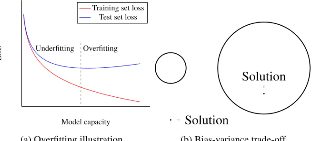
The ability of the model to represent different configuration is the model’s capacityand in simple cases it is just the number of the parameters |Θ|, computed up to all possible parameter symmetry. Additionally, capacity reduces with any kind of constraint, soft or a hard one. The bigger capacity, the richer the space of prediction functions representable by the model. It means that a model with small capacity does not have enough flexibility to represent the training data, assign the right class for the majority of the data for classification task. As soon as the model capacity is too high, it specializes on the training data which leads to the degradation of the test score. This behaviour is depicted on the Figure 2.1a: the low capacity regime is called underfitting and the high capacity regime is overfitting. The ideal model is one on the dashed line, with minimal test error rate. This is connected to the bias and variance of the statistical estimator, and thus
called bias-variance trad-off, it is illustrated on the Figure 2.1b, the left picture demonstrates a small family of functions which corresponds to low capacity, low variance and high bias; and the right picture demonstrates the case of high capacity and high variance.
For this purpose we maintain a separate test set which is used for scoring. Unfortunately, the process of searching a model and its configuration (also called hyper-parameter search) is also a learning task which can be prone to overfitting. To solve this issue, we introduce one more set: cross-validation set which should be used for the hyper-parameter tuning and model search. Ideally, in order to avoid overfitting on the test set, the model should be evaluated on the test set only once.
Some of the methods for capacity control for the model, the regularization techniques discussed in the Section 2.2.2.
Underfitting
Underfitting Overfitting
Model capacity
Loss
Training set loss Test set loss
(a) Overfitting illustration.
.
Solution
.
Solution
(b) Bias-variance trade-off.
Figure 2.1: Overfitting example. This is an illustration of a model accuracy on the training and the test sets depending on the model capacity. With a limited capacity model is not able to capture the data dependencies and its performance is bad on both test and training sets. With an increase of capacity the performance increases then the test loss stops improving while the training loss continues to go towards zero. The first region is the underfitting, the model is not able to fit the data; and the second is overfitting, the model is so powerful that it fits the particular characteristics of the training data which does not exist in the test set.
2.2
Deep Learning
When the field is field of machine learning is new and fast moving, deep learn-ingis even more so.
One of a successful models nowadays are variations of neural networks. The neural networks are compositional functions
f(x) = fK( fK−1(· · · f1(x))), (2.2)
which consist of K differentiable functions f1, . . . , fK, or in some cases almost
ev-erywhere differentiable (like rectified linear nonlinearities, which are introduced below).
The simplest example of a neural network is a logistic regression. It is mistak-enly called “regression”, though it solves a classification task. The model is very simple: first, the input features are linearly transformed
h= W x, (2.3)
where the matrix of parameters W has the dimensionality of |Y | × |X |. Then the transformed features are put through the softmax function
ˆ
y= softmax(h) = exp h ∑jexp hj
. (2.4)
The softmax function is a generalization of a sigmoid function
σ(h) = 1
1 + exp(−h), (2.5)
which is applicable for a scalar h and is used to represent how probable the positive class is. The ˆy can be considered as an estimated probability distribution over the output classes. Finally, the cross-entropy with the ground truth answer is computed as
L( ˆy, y) =
∑
j
yjln ˆyj. (2.6)
Here we assume that the ground truth is represented as a one-hot vector, mean-ing that y is a vector with a number of elements equals to a number of classes containing zeros in all positions except for a one in a position of the ground truth class.
The neural network terminology often uses layers as building blocks, in the multiclass logistic regression example there is only two layers: a linear layer and
a softmax layer. Often a linear and a succeeding nonlinearity are referred as a single layer. More complicated networks stack more layers on top of each other.
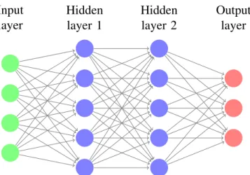
Feed-forward networks or multi-layer perceptrons (MLP) are very similar to the logistic regression but include more layers of linear transformation followed by nonlinearities before applying the final softmax layer. Figure 2.2 demonstrates a computation flow graph for a two layer MLP. More complicated models may involve more complicated computation flow and the requirement is that the com-putation graph should be a directed acyclic graph (DAG). In this case the output can be computed given inputs. The more layers network has the deeper it is, the effect of the depth on the ability to represent diverse function and the regulariza-tion will be discussed below.
The nonlinearities is an essential part of deep neural networks since stacking more than one linear layer is equivalent to having a single one. Historically, a sigmoid nonlinearity was very popular due to several factors, it can be interpreted as a probability of having some hidden feature; it is biologically plausible in some sense; the sigmoid networks can pre-trained in layer-wise manner using restricted Boltzmann machines (RBM) with binary units. Nowadays, the importance of pre-training it not so high due to development of computational resources such as graphical processing units (GPU), availability of the optimized implementations of linear algebra operations (cuBLAS, cuDNN), and innovations in the optimiza-tion which will be discussed in the Secoptimiza-tion 2.2.1. These and many other factors resulted into number of research papers on investigation of different kinds of non-linearities. The most frequently used ones are
• Sigmoid element-wise nonlinearity is difficult to train due to saturation ef-fects.
• It is used to ensure that the output is constrained to be in the region [0, 1] or to model the Bernoulli distribution
g(x) = σ(x). (2.7)
• Rectified linear units (ReLU) are successfully used in the context of convo-lutional neural networks (CNN) for image processing tasks and fully con-nected networks, but there is some work concerning applications of ReLUs for RNNs which concludes that a careful initialization is needed
• MaxOut units [48] is a generalization of rectified units and basically sepa-rate the output space into several linear regions
gi(x) = max
j∈[1,k]{x TW
·i j+ bi j} (2.9)
• The hyperbolic tangent (tanh) nonlinearity mostly used for the recurrent neural networks, see Section 2.2.4
g(x) = tanh x. (2.10)
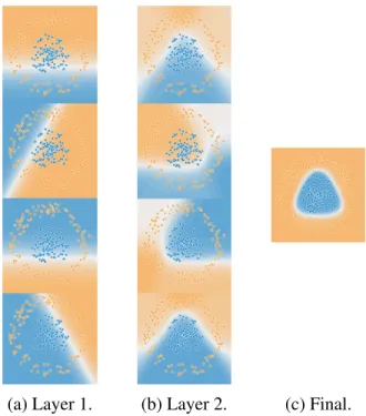
Constructing deeper networks help learning better representations and many studies show that lower layers learn simple features like linear edge detectors when higher layers combine the features received from previous layers and con-struct more complex representations like circle detectors and even face detectors or animal detectors [83]. This is shown1 for a toy task in Figure 2.3. The task is two class separation where the fist class data points are sampled uniformly in the inner circle and the second class is sampled in the ring outside the circle. This task cannot be solved using linear classifiers since there is no linear boundary sep-arating the classes and here we used a two layer MLP with 4 hidden units in each layer and tanh nonlinearities everywhere. The graph shows the decision bound-ary reprojected to the input space for every hidden neuron and the final decision boundary for the whole classifier. It is clear that the first layer (Figure 2.3a) learns simple linear boundaries, the second layer (Figure 2.3b) learns more complicated representations with simple curves, and the softmax output (Figure 2.3c) is able to combine it to produce the high quality decision boundary.
This makes deep neural networks to become a step towards end-to-end learn-ing since the feature representations are trained from data and no handcraftlearn-ing is required.
2.2.1
Optimization
In this section we briefly discuss optimization with focus for neural networks. The neural networks were developed to be easily optimized using gradient methods, the main idea is using the chain rule
∂ fi(g(x)) ∂xj =
∑
k ∂ fi(g(x)) ∂gk(x) ∂gk(x) ∂xj , (2.11)1Special credits to the tensorflow team and the tensorflow playground:https://playground.
Hidden layer 1 Hidden layer 2 Input layer Output layer
Figure 2.2: Example of a two hidden layer neural network. The input size is 4, both hidden layers have size 5 and the output is 3 (which is the number of output classes). This is a computation flow directed acyclic graph (DAG). More compli-cated neural network models may have more complicompli-cated computation flow as far as it can be represented with and a graph without cycles.
where f and g are vector functions of a vector argument x. Since a neural network is a composition of many differentiable functions the chain rule can be applied for every composition recursively. The efficient algorithm to compute the gradient is an obvious case of dynamic programming: during forward pass we compute all the activations (intermediate function results) then in a backward pass we compute the gradient using the chain rule and the stored activation from the forward pass. Notice, that this algorithm can be applied to a matrix input x, where the matrix is the batch of inputs.
Now, we are able to compute the gradient and the easiest way to optimize a network is using stochastic gradient descent (SGD). A mini-batch of examples is sampled from the training set, the gradient of the loss is computed using the back-propagation algorithm and the parameters are updated as
θ(t+1)i = θ(t)i − α∂L( ˆy, y) ∂θ(t)i
, (2.12)
where α is the learning rate.
There exist more sophisticated optimization methods which estimate the Hes-sian diagonal such as RMSProp, AdaGrad, ADADELTA [173], Adam [78].
(a) Layer 1. (b) Layer 2. (c) Final.
Figure 2.3: Decision boundaries for a two layer network trained on a toy data. Points from the first class are surrounded by points from the other class which makes this task impossible to solve using linear classifiers but can be easily solved after around 200 iterations of the gradient descend.
2.2.2
Regularization
The overfitting problem discussed in the Section 2.1.2 requires to use regular-ization to reduce the capacity of the model.
One of the most successful methods for neural network models is dropout. It randomly turns off neurons of the network with some constant probability, the common choice is 50% for the hidden neurons and 80% for the input ones, but it may be task dependent. The dropout prevents co-adaptation of the neurons and enforces over-representation making the network more robust to small perturba-tions of the input.
In our work we also used a weight matrix norm constraint regularization method. This was crucial to use it sophisticated recurrent models (Section 2.2.4) for large vocabulary speech recognition models reported in the Section 2.4.
The weight noise, and in particular, the adaptive weight noise [50] is a method which uses the variational inference ideas for regularizing recurrent neural net-works was used to achieve the state of the art on small speech corpora like TIMIT. This method sets up the Gaussian prior over the weight matrices elements and per-forms sampling. In other words, random Gaussian noise is added to the weights. In the case of the adaptive weight noise, the mean and the variance of the Gaussian are trainable parameters.
2.2.3
Autoregressive Models
Distributions modelling complex real world systems generally require a lot of factors. When every such factor corresponds to a variable in the distribution, the dimensionality of the input is substantial. This especially true for streams of data, strings, time series. These structures are potentially infinite therefore they require infinite dimensional input. However, an intuition tells us that every observation in the series does not depend on the future observations. In other words, when modelling a given observation, we need to take into consideration only previous observations. Models that work this way are called autoregressive models.
Putting into math the intuition in the previous paragraph, we look at a distribu-tion of a sequence of random variables y1, . . . , yT. Any multi-variable distribution
p(y1, . . . , yT) can be factorized as
p(y1, . . . , yT) = p(y1)p(y2|y1) . . . p(yT|y1, . . . , yT−1) = p(y1) T
∏
t=2
p(yt|y1, . . . , yt−1),
or using notation y<i= {y1, . . . , yi−1}, p(y1, . . . , yT) = p(y1) T
∏
t=2 p(yt|y<t). (2.14)This is also true for a model distribution q(y1, . . . , yT)
q(y1, . . . , yT) = q(y1) T
∏
t=2
q(yt|q<t). (2.15)
Writing down the Kullback-Leibler divergence between distributions p and q DKL(p||q) = −H(p) − Eplog q(y1) +
T
∑
t=2
log q(yt|q<t), (2.16)
where H(p) is the entropy of the data distribution p that is constant, therefore does not affect optimization. Minimization of the Kullback-Leibler divergence corresponds to minimization of the second term which is called the cross-entropy between p and q. An important observation is that the cross-entropy of the factor-ized distribution is the sum of conditional cross-entropies
H(p, q) = H (p(y1), q(y1)) + T
∑
t=2
H(p(yt|y<t), q(yt|y<t)) . (2.17)
In practice, it is intractable to perform the summation over all the inputs. Fur-thermore, data distribution p is unknown in most practical cases, we are given only samples from this distribution. To tackle these two issues, we make a single sample approximation of the expectation
Eplog q(y1, . . . , yT) ≈ log q(y01, . . . , y0T), (2.18)
where y01, . . . , y0T ∼ p(y1, . . . , yT) a sample from the data distribution p. Basically,
this means that we can have an estimate of the cross-entropy simply sampling a single point from the dataset. Combining this approximation with the Equa-tion 2.17 H(p, q) ≈ − log q(y01) − T
∑
t=2 log q(y0t|y0<t). (2.19) In other words, we use a sample from the dataset to guide the prediction. Then, at every t we make a one step ahead prediction. This procedure is know as teacherforcing algorithm because the sequence we condition on y0<t is forced to be a sample from the dataset.
When performing inference, most commonly we use ancestral sampling from the learned distribution q. In other words, we sample the y01from q(y1), then every
yt from q(yt|y0<t), where the conditioning part notation means that the all variables
before t are clamped to previously sampled y01, . . . , y0t−1.
While this is straightforward on the paper, in practice it can lead to problems. This class of problems is a kind of over-fitting (see Section 2.2.2) and is called exposure bias[121]. The exposure bias problem might affect any autoregressive model, but first was discovered in the context of recurrent neural networks (see Section 2.2.4). The origin of the exposure bias is that the training procedure is substantially different from the inference procedure. During the training, we see only the correct samples from the dataset, while during the inference, the model is conditioned on the samples from the model itself. Even for very accurate models the probability of making a mistake in a long sequence is growing exponentially. In other words, even if the probability of making a mistake at any given time-step is as low as ε, the probability of making a mistake in a sequence of length T is 1 − (1 − ε)T. After making a single mistake during the inference, the model can find itself in the state which it has never encountered during the training. Because of this, the model starts to wander off the familiar path and produce worse and worse mistake.
The exposure bias problem has been studied from different aspects. The pro-posed solutions range from approaches based on reinforcement learning based data as demonstrator [160], SEARN [35], dataset aggregation [125]. Other works apply REINFORCE algorithm [163] to sequence prediction problems [54]. A downside of the reinforcement learning approaches is that, usually, the gradient has high variance. Another set of approaches tries to bring closer the training stage to the inference. The examples are scheduled sampling [16], where randomly cho-sen tokens are sampled from the model distribution instead of the dataset; profes-sor forcing[87], where a generative adversarial network is used to close the gap between the training and testing.
Besides the exposure bias, autoregressive models frequently have difficulties generating long consistent sequences. This is discussed in Section 2.2.5 in the context of recurrent neural networks.
2.2.4
Recurrent Neural Networks
For the tasks which have temporal structure we need to deal with the sequences which potentially have variable length. This type of networks is referred as the recurrent neural networks (RNNs). The simplest RNN takes the input and the previous state to produce a new state
ht= g(Wxhxt+ Whhht−1+ bh), (2.20)
where g is a nonlinearity function, often a hyperbolic tangent; xt is the input at
the time step t, ht−1 is the previous hidden states; and Wxh, Whh, bh are the
parameters, input-to-hidden, hidden-to-hidden matrices and the bias respectively. The RNNs can be used in two scenarios: whether for generation or for feature representation. A generative RNNs models a distribution
p(y1, . . . , yT) = p(y1)p(y2|y1) · · · p(yT|y1, . . . , yT−1) (2.21)
aggregating the information required for the conditioning in the state variable. The second scenario is a feature representation for the temporal information. In this case the representation and the output is the tensor of the hidden states.
In both these cases the function computed by the RNN is differentiable, so the derivative with respect to the parameters can be computed using the propagation algorithm on a unfolded RNN, this algorithm is referred as back-propagation through time(BPTT).
2.2.5
Long Short-Term Memory recurrent networks
A particularly successful recurrent neural network architecture is the Long Short-Term Memory (LSTM) [71]. The LSTM is designed to handle long-term dependencies by gating the information that enters and leaves its so-called mem-ory cells using multiplicative gating units. The hidden states of a commonly used LSTM variant [52] are computed using the following set of equations:
it = σ(Wxixt+ Whiht−1+ Wcict−1+ bi)
ft = σ(Wx fxt+ Wh fht−1+ Wc fct−1+ bf)
ct = ft⊗ ct−1+ it⊗ tanh(Wxcxt+ Whcht−1+ bc)
ot = σ(Wxoxt+ Whoht−1+ Wcoct+ bf)
where i, f and o represent the input, forget and output gates and c contains the values of the memory cells. The symbol ⊗ signifies element-wise multiplication. The matrices Wci, Wc f and Wcoare constrained to be diagonal.
Another variant is Gated Recurrent Units (GRU, [33]) which was designed to be more computationally efficient than LSTM units as it has a simpler architec-ture [31]. The hidden states htare computed using the following equations:
zt = σ(Wxzxt+ Uhzht−1),
rt = σ (Wxrxt+ Uhrht−1) ,
˜ht = tanh (Wxhxt+ Urh(rt⊗ ht−1)) ,
ht = (1 − zt)ht−1+ zt˜ht,
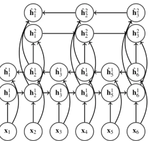
The networks introduced above can only aggregate the information in one direction. Sometimes the features at time step t depend on the future information and for this purpose two recurrent networks can be run in opposite directions and their states concatenated. This type of recurrent networks is often referred as the bidirectional RNNs (BiRNN). Obviously, not only can simple RNNs be bidirectional, one can construct bidirectional LSTMs and GRUs using their hidden states.
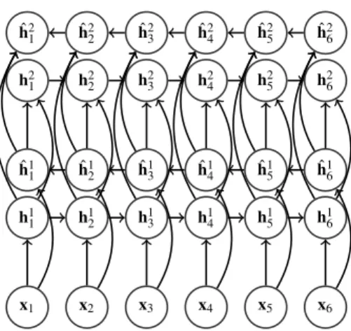
Frequently, one more trick is used to obtain a better representation: stacking several RNNs on top of each other like it is done in deep neural networks. It has been shown that one can pass the data through several layers of RNNs to obtain better performance for speech recognition in [56]. It is done simply considering the output sequence h1, . . . , hT of the states of the first layer as the input to the
second one. The Figure 2.4 illustrates two simple bidirectional networks stacked on top of each other.
2.2.6
Sequence Generation with Recurrent Neural Networks
The tasks like speech recognition involve inputs and outputs having variable length. Therefore the input should be aligned to the output, which is a complicated chicken-and-egg type of learning problem. The model may need a good alignment to produce good classification results but there is no way to figure the alignment without a classification model. For speech recognition models the Hidden Markov Model is usually used and will be discussed in the Section 2.3.1.
The idea to train the model to align and perform its task simultaneously origi-nated to the machine translation community in a context of encoder-decoder net-works [27, 150]. The encoder network is used to generate an intermediate
rep-h2 1 h22 h23 h24 h25 h26 ˆh2 1 ˆh22 ˆh23 ˆh24 ˆh25 ˆh26 ˆh1 1 ˆh12 ˆh13 ˆh14 ˆh15 ˆh16 h1 1 h12 h13 h14 h15 h16 x1 x2 x3 x4 x5 x6
Figure 2.4: Two Bidirectional Recurrent Neural Networks stacked on top of each other.
resentation which is passed to the decoder network which is typically an RNN working as a generative one as described in Section 2.2.4.
A simple encoder-decoder is supposed to save a whole input sequence to a fixed dimension vector to pass it to the decoder. This is not feasible for some applications having long sequences as the handwritten text generating. This was addressed in [52] and a kind of attention was proposed which used several Gaus-sian windows averaging over the time dimension to select the information needed for every generation step.
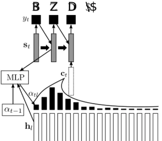
The Attention-based Recurrent Sequence Generators (ARSG [8]) uses a more general approach to the attention. The ARSG produces the output sequence y1, . . . , yT
one element at a time using the state information and simultaneously aligning the generated element to the input sequence h1, . . . , hL produced by the encoder. The
encoder usually is a stack of bidirectional recurrent networks (LSTMs or GRUs). The elements are “selected” from the input sequence like
ct =
∑
lαtlhl, (2.22)
where the αtl are the attention weights produced by an attention mechanism. See
Figure 2.5 for a schematic representation of an ARSG.
work-B Z D $
Figure 2.5: A schematic illustration of an attention mechanism network. Every frame in the encoded input hl is weighted by an MLP which depends on this
frame, previous hidden state of the generator and the previous time step attention weights. This makes this particular attention content and position based attention. The output is sampled conditioned on the ground truth previous character during training and on the previously sampled character during testing.
ing as follows F = Q ∗ αt−1 (2.23) etl = w>tanh(Wst−1+ Vhl+ Ufl+ b) (2.24) αtl = exp(etl) L ∑ l=1 exp(etl) . (2.25)
where W, V, U, Q are parameter matrices, w and b are parameter vectors, ∗ denotes convolution, st−1stands for the previous state of the RNN component of
the ARSG. We explain how it works starting from the end: (2.25) shows how the weights αtl are obtained by normalizing the scores etl. As illustrated by (2.24),
the score depends on the previous state st−1, the content in the respective location
hland the vector of so-called convolutional features fl. The name “convolutional”
comes from the convolution along the time axis used in (2.23) to compute the matrix F that comprises all feature vectors fl.
Different types of attention were used for machine translation [8], caption generation [164] and phoneme-level speech recognition [29].
2.3
Automatic Speech Recognition
This section briefly summarizes previous work on automatic speech recog-nition (ASR). We start with description of the hybrid speech recognizes in tion 2.3.1 and continue with the discussion of the end-to-end systems in the Sec-tion 2.3.2.
2.3.1
Hybrid Systems
Widely used type of ASR systems is hybrid speech recognition systems, they combine several components into one pipeline and every component is optimized separately [41]. First step, feature extraction, is performed using signal processing techniques is discussed in Section 2.3.1. The processed features are the inputs for the acoustic model represented by some kind of a phone classifier (Gaussian Mixture model, deep neural network [67], or recurrent neural network [56]), it is trained to assign a phone for every time frame. It is discussed more in the Section 2.3.1. Then a pronunciation model which is frequently a hidden Markov model is trained to transform the phonemes to the output sequence, it is explained in the Section 2.3.1. Finally, the acoustic model is combined with an external language model, see Section 2.3.1.
An ASR system is modelling the probability of a sequence of words y1, . . . , yL
given an input sequence of acoustic vectors x1, . . . , xT [21] which can be factorized
in the following way
p(y|x) ∝ p(x|y)p(y) = p(x|s)p(s|y)p(y), (2.26) where s is the pronunciation (or sounding). And in order to solve the speech recognition task one has to find the most probable sequence of outputs
ˆ
y= arg max
y,s
p(x|s)p(s|y)p(y), (2.27)
maximizing over all possible pronunciation and the outputs. Three multiplier at the right hand side represent three main parts of an ASR system p(y) is the lan-guage model; p(x|s) is the pronunciation model and p(x|s) is the acoustic model. Feature Extraction
The most popular way to preform the feature processing of the raw audio sig-nal is to extract so-called mel-frequency cepstral coefficients or MFCCs and its
first and second derivatives. MFCCs can be computed using following proce-dure [1]:
• First, the Fourier transform of the raw signal divided into intersecting win-dows is taken.
• The powers of the spectrum obtained after the Fourier transform is mapped onto the mel scale using triangular overlapping windows.
• The logarithms of the powers at each of the mel frequencies are computed. • The discrete cosine transform of the list of mel log powers is performed, as
if it were a signal.
• The MFCCs are computed as the amplitudes of the resulting spectrum. Phoneme Recognition
The acoustic model perhaps is the hardest part in terms of training difficulty of the ASR system. The initial alignment is obtained running Baum-Welch algorithm with the GMM-HMM model (the Hidden Markov models for pronunciation are discussed in Section 2.3.1). This algorithm is a particular case of the expectation-maximization (EM) algorithm. Then a more complicated DNN or RNN acoustic model is trained with this pre-trained alignment.
The acoustic model is trained to model the p(x|s) distribution from the Equa-tion (2.27). And the pronunciaEqua-tion is supposed to consist from the phones (atomic sounds in the language), which construct phonemes, constrained by the lexicon. Hidden Markov Models
A popular for many tasks hidden Markov model is used for the pronunciation model in hybrid ASR systems. This model is basically is stochastic finite automa-ton and received its name due to that the observable stochastic process is modelled with an assumption of having some hidden states. The inference in the HMM is performed using the efficient dynamic programming Viterbi algorithm.
Hidden Markov models used in ASR are used in a concatenation of several final state transducers (FST). First, the context-dependency transducer is con-structed. This FST is concatenated with the hidden Markov model, then with the pronunciation FST which maps the words to their pronunciations. This FST
Figure 2.6: A simple weighted finite state transducer. It has three states, 0 is the initial state and 1 is the accepting state. Both the input and the output has the vocabulary of {0, 1, 2, 3}. Every transition is marked as input:output/weight.
is concatenated with the grammar transducer (or the language model, see Sec-tion 2.3.1). The hidden Markov model is trained to map from the transiSec-tion-ids to the context-dependent frames.
Language Models
Most commonly used language models in ASR systems are N-gram language models, although the state of the art was achieved with a deep RNN language model in many tasks [100].
An efficient implementation of the N-gram language models uses the weighted finite state transducers(wFST; [3, 102]) and it makes the N-gram LM compatible with the pronunciation HMM represented as a stochastic finite state automaton. See Figure 2.6 for an example of a simple wFST. These two models can be com-bined using simple wFST operation of concatenation. Other standard operations are used to minimize the resulting transducer and to push the weights toward the initial state to help the beam search.
In the case when the RNN LM is used it is not possible to use the wFST machinery to get the concatenated acoustic and the LM transducer. A common approach in this case and sometimes with the N-gram models as well is to produce a lattice and re-weight it with the LM. Basically, the lattice is the augmented result of the beam search algorithm run on the decoding wFST, it is the set of the paths obtained from the beam search after merging the same states.
2.3.2
End-to-end Systems
End-to-end systems recently proposed for the ASR. The connectionist tem-poral classification [53] uses the dynamic programming algorithm to construct a differentiable loss which integrates out the alignment of the input and the output.
This is performed adding a new token to the output vocabulary for the blank out-put and this token is ignored when constructing the outout-put. Later work [54] uses the same CTC cost to construct a model which optimizes the task loss again, us-ing the dynamic programmus-ing and a type of the REINFORCE algorithm. One of the problems of the CTC-based models that it does not learn the internal language model due to the absence of the output RNN. This was solved with the neural transducers [51] which use the same idea of dynamic programming but include the output RNN. The disadvantage of the neural transducer is that it is computa-tionally expensive to train.
2.4
End-to-end Large Vocabulary Speech
Recogni-tion
This section summarizes work on adaptation of attention-based architectures which brings us closer to the end-to-end speech recognition on large vocabulary datasets, published in [9]. This model is one of the crucial components for the experiments outlined in Chapter 4 and an inspiration for the work presented in Chapter 5.
2.4.1
Introduction
Several successful works on end-to-end large vocabulary automatic speech recognition include [98, 64, 63], which used CTC-based architectures for LVSR tasks like Wall Street Journal dataset and Switchboard dataset.
The work [9] builds up on the works [28, 29] on investigation ARSGs 2.2.6 for speech recognition and provides experimentation on a bigger Wall Street Journal speech corpora. The tree main contributions of this work are the following. First, the paper shows how training on long sequences can be made feasible by limiting the area explored by the attention to a range of most promising locations. This reduces the total training complexity from quadratic to linear, largely solving the scalability issue of the approach. This has already been proposed [29] under the name “windowing”, but was used only at the decoding stage in that work. Sec-ond, in the spirit of the Clockwork RNN [82] and hierarchical gating RNN [33], the paper introduces a recurrent architecture that successively reduces source se-quence length by pooling frames neighboring in time. This mechanism has been independently proposed in [23].
Finally, the paper shows how a character-level ARSG 2.2.6 and N−gram word-level language model can be combined into a complete system using the weighted finite finite transducers(wFST) framework.
2.4.2
Model for Large Vocabulary Speech Recognition
The work uses an attention-based sequence generation model introduced in the Section 2.2.6. The encoder network is a multilayer bidirectional RNN (see Section 2.2.5) and uses one more trick to speed up the computation: pooling along the time dimension. In a nutshell, the paper provides only every k frames to the succeeding layer of a recurrent network, see the Figure 2.7 for the details. In the