Science Arts & Métiers (SAM)
is an open access repository that collects the work of Arts et Métiers Institute of Technology researchers and makes it freely available over the web where possible.
This is an author-deposited version published in: https://sam.ensam.eu Handle ID: .http://hdl.handle.net/10985/10211
To cite this version :
Abdellah SALAHOUELHADJ, Farid ABED-MERAIM, Hocine CHALAL, Tudor BALAN - On the implementation of the continuum shell finite element SHB8PS and application to sheet forming simulation - American Institute of Physics Conf. Proc. - Vol. 1353, p.1203-1208 - 2011
Any correspondence concerning this service should be sent to the repository Administrator : [email protected]
On the implementation of the continuum shell finite element
SHB8PS and application to sheet forming simulation
A. Salahouelhadj, F. Abed-Meraim, H. Chalal and T. Balan
Laboratoire d'Etude des Microstructures et de Mécanique des Matériaux, LEM3 - UMR CNRS 7239 Arts et Métiers ParisTech─Metz
4 rue A. Fresnel, 57078 Metz Cedex 03, France
Abstract. In this contribution, the formulation of the SHB8PS continuum shell finite element is extended to anisotropic elastic–plastic behavior models with combined isotropic-kinematic hardening at large deformations. The resulting element is then implemented into the commercial implicit finite element code Abaqus/Standard via the UEL subroutine. The SHB8PS element is an eight-node, three-dimensional brick with displacements as the only degrees of freedom and a preferential direction called the thickness. A reduced integration scheme is adopted using an arbitrary number of integration points along the thickness direction and only one integration point in the other directions. The hourglass modes due to this reduced integration are controlled using a physical stabilization technique together with an assumed strain method for the elimination of locking. Therefore, the element can be used to model thin structures while providing an accurate description of the various through-thickness phenomena. Its performance is assessed through several applications involving different types of non-linearities: geometric, material and that induced by contact. Particular attention is given to springback prediction for a NUMISHEET benchmark problem.
Keywords: solid–shell element, reduced integration, physical stabilization, assumed strain method, elastic–plastic behavior, sheet metal forming, springback.
PACS: 02.70.Dh
1. INTRODUCTION
During the last decade, considerable effort has been devoted to the development of eight-node solid–shell elements for modeling of thin structures (e.g. [1-4]). As they use linear interpolation for efficiency reasons, these elements exhibit various locking phenomena which need to be cured in order to preserve the desired accuracy. Nevertheless, compared to conventional shell elements they have many advantages: the use of full three-dimensional constitutive laws, direct calculation of thickness variations, easy treatment to update configurations (no rotational degrees of freedom used), and simple connection with three-dimensional elements since displacements are the only degrees of freedom. For sheet forming applications, key features like double-sided contact and increased accuracy with only one layer of elements through the thickness make these elements particularly attractive.
The reduced integration technique, initiated by the works of Zienkiewicz et al. [5] and Hughes et al. [6], was the first successful solution to alleviate some locking pathologies. Finite elements using this method are very efficient due to their low numerical cost. However, stabilization techniques are needed in order to control the spurious zero-energy deformation modes (or hourglass modes) induced by this reduced integration.
In order to circumvent locking phenomena for three-dimensional low-order elements, several authors have used the enhanced assumed strain (EAS) method, based on Simo and Rifai's pioneer work [7]. The basis of such element formulations is given by the mixed variational principle in which the so-called incompatible strain and stress act as additional independent variables. Recent investigations have combined EAS and reduced integration techniques to derive efficient and accurate elements. As examples, some authors used a fixed number of Gauss points in the thickness direction [1-4].
The SHB8PS is one such element that has been recently developed [1, 2], based on in-plane one-point numerical quadrature with eight physical nodes and using an arbitrary number of integration points through the thickness direction. This avoids the use of several layers of elements in order to increase the number of integration points in
the thickness, e.g. for metal forming problems. The hourglass modes caused by this reduced integration are efficiently controlled by a physical stabilization technique based on the assumed strain method [8].
In the current contribution, the formulation of the SHB8PS solid–shell finite element is extended to anisotropic elastic–plastic behavior models with combined isotropic-kinematic hardening at large deformations. The resulting element is then implemented into the commercial implicit finite element code Abaqus/Standard via the UEL subroutine. Its good performance is demonstrated through non-linear benchmark problems involving large strains, plasticity and contact. Particular attention is given to springback prediction for a NUMISHEET benchmark problem.
2. FORMULATION OF THE SHB8PS ELEMENT
2.1. Finite element interpolation
SHB8PS is an eight-node, isoparametric hexahedral element with linear interpolation. It has a set of nint
integration points chosen along the thickness direction
ζ
in the local coordinate frame (see Fig.1).FIGURE 1. SHB8PS reference geometry.
The spatial coordinates xi and displacements ui of any point in the element are related to the nodal coordinates
and nodal displacements xiI and uiI, respectively, using the classic linear isoparametric shape functions NI:
8 1 ( , , ) ( , , ) i iI I iI I I x x N ξ η ζ x N
ξ η ζ
= = =∑
(1) 8 1 ( , , ) ( , , ) i iI I iI I I u u N ξ η ζ u Nξ η ζ
= = =∑
(2)Subscript i varies from 1 to 3 and represents the direction of the spatial coordinates. Subscript I varies from 1 to 8.
2.2. Discretized gradient operator
First, we introduce the bi (i = 1,..., 3) vectors, representing the derivatives of the shape functions at the origin of the reference coordinate system, defined by Hallquist [9] as
, (0, 0, 0) 1, 2, 3 T
i i
b =N i= (3)
The displacement gradient can then be written as follows (see Belytschko and Bindeman [8]):
(
)
4 , , , 1 T T T T i j j j i j j i u b hα α d b hα α d αγ
γ
= =⎛
⎜
+⎞
⎟
⋅ = + ⋅⎝
∑
⎠
(4)where diare the nodal displacement vectors. The functions
h
α and vectors γ (α=1,...,4) are given by α1 , , , 2 3 4
3 1 1 ( ) 8 T j j j h h x b α α α γ = =
⎡
⎢
− ⋅⎤
⎥
⎣
∑
⎦
(6)The discretized gradient operator can be written as
, , , , , , , , , 0 0 0 0 0 0 0 0 0 T T x x T T y y T T z z T T T T y y x x T T T T z z y y T T T T z z x x b h b h b h B b h b h b h b h b h b h α α α α α α α α α α α α α α α α α α
γ
γ
γ
γ
γ
γ
γ
γ
γ
+ + + = + + + + + +⎡
⎤
⎢
⎥
⎢
⎥
⎢
⎥
⎢
⎥
⎢
⎥
⎢
⎥
⎢
⎥
⎢
⎥
⎣
⎦
(7)2.3. Stabilization and assumed strain method
The particular location of the integration points along a line generates six so-called hourglass modes. The control of the hourglass modes of the SHB8PS element is achieved by adding a stabilization component KSTAB to the element stiffness matrix Ke. This part is drawn from the work of Belytschko and Bindeman [8], who applied an efficient stabilization technique together with an assumed strain method. The stabilization forces are consistently derived in the same way. Moreover, the discretized gradient operator is projected onto an appropriate sub-space in order to eliminate shear and membrane locking.
In this approach, the bi vectors (Eq. (3)) are replaced by the mean value of the derivatives of the shape functions over the element, denoted by bˆi , as proposed by Flanagan and Belytschko [10]:
, 1 ˆ ( , , ) , 1, 2, 3 e e T i i b N ξ η ζ d i Ω Ω =
∫
Ω = (8)Then, vectors
γ
α are replaced by vectorsγ
ˆα where the bi vectors are simply substituted by bˆi . A modified discretized gradient operator ˆB can be constructed in the same way. It can be shown that the terms of the ˆB operator vanish for α=3,4. In other words, the ˆB operator reduces to its ˆB12 part defined identically but where α varies only from 1 to 2. Then, the remaining part ˆB34 of ˆB, which vanishes at the integration points, is further projected as ˆB34. One can project the ˆB operator onto a ˆB operator as:12 34
ˆ ˆ ˆ
B =B +B (9)
where ˆB34 is given by:
4 , 3 4 , 3 3, 3 34 4, 4 ˆ 0 0 ˆ 0 0 ˆ 0 0 ˆ 0 0 0 0 0 0 ˆ 0 0 T x T y T z T x h h h B h α α α α α α
γ
γ
γ
γ
= = =⎡
⎤
⎢
⎥
⎢
⎥
⎢
⎥
⎢
⎥
⎢
⎥
⎢
⎥
⎢
⎥
⎣
⎦
∑
∑
(10)The stiffness matrix Ke takes the form:
12
ˆ ˆ
e
T
e Geom STAB Geom
ep
K B C B d K K K K
Ω
=
∫
⋅ ⋅ Ω + = ++
(11)where the first term K12 is evaluated at the integration points as
int 12 12 12 12 12 1 ˆ ˆ ( ) ( )ˆ ( ) ˆ ( ) e n T T ep I I I I I ep K B C B d
ω ζ
Jζ
Bζ
C Bζ
= Ω =∫
⋅ ⋅ Ω=
∑
⋅ ⋅ (12)In this equation, J
( )
ζ is the Jacobian of the transformation between the reference and the current configurations; I( )I
ω ζ
is the corresponding weight, while epC σ
ε
∂∆ =
∂∆ is the elastic–plastic tangent modulus. The geometric stiffness matrix KGeom is due to the non-linear (quadratic) part of the strain tensor and KSTAB represents the stabilization stiffness given by equation:
12 34 34 12 34 34 ˆ ˆ ˆ ˆ ˆ ˆ e e e T ep T ep T ep STAB K B C B d B C B d B C B d Ω Ω Ω =
∫
⋅ ⋅ Ω +∫
⋅ ⋅ Ω +∫
⋅ ⋅ Ω (13)In a similar way, the internal forces of the element can be written as
int 1 12 ˆ ( ) ( ) ( ) ( ) n STAB I I I I I T int f
ω ζ
Jζ
Bζ
σ ζ
f = =∑
⋅ + (14)where fSTAB represents the stabilization forces.
The stabilization terms are calculated in a co-rotational coordinate system [8].
3. NUMERICAL EXAMPLE: UNCONSTRAINED CYLINDRICAL BENDING
The example of the unconstrained cylindrical bending test proposed as springback benchmark in NUMISHEET 2002 is studied [11]. This application allows us to evaluate the performance of the SHB8PS element , implemented in Abaqus/Standard, in presence of geometric, material and contact non-linearities. This benchmark involves a bending-dominated deformation since there is no blank holder. The problem has complex contact boundary conditions during the forming process and the springback after forming is severe. The geometry of the problem is illustrated in Fig.2 and the geometric parameters are summarized in Table 1.
The material under investigation is a High Strength Steel, which is supposed elastic–plastic with isotropic hardening following Swift law:
(
0)
Y n P eqK
σ
=ε
+
ε
(15)where K,ε0andn represent the material parameters and P eq
ε is the equivalent plastic strain. The Young modulus
5
E = 2.175 × 10 MPa and the Poisson ration ν = 0.3. Further K = 645.24, n = 0.25177 and ε0 = 0.0102. The friction
coefficient of the interaction between surfaces punch-sheet and die-sheet is µ = 0.14812.
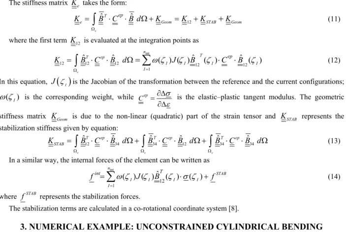
The amount of springback is quantified by the angle θ as defined in Fig.3. This angle is measured after forming at the maximum punch displacement and after springback. The tools are defined as analytical rigid surfaces.
TABLE 1. Geometric parameters of the unconstrained cylindrical bending problem
Geometric parameter [mm] Geometric parameter [mm]
Punch radius 23.5 Length of the sheet 120.0 Die radius (R2) 25.0 Thickness of the sheet 1.0 Die shoulder (R3) 4.0 Width of the sheet 30.0 Width of tools (W) 50.0 Punch stroke 28.5
FIGURE 3. Definition of the angle to measure springback for the unconstrained cylindrical bending problem
The SHB8PS element is compared with both solid and shell elements. Indeed, it is well-known that in applications of sheet metal forming, shell elements have difficulties in dealing with double-sided contact – while conventional solid elements require several element layers to capture bending effects. In the present work, the simulations carried out with the SHB8PS element use only one element layer through the thickness. For symmetry reasons, only one quarter of the blank is discretized by means of 150 SHB8PS elements in the length and only one element over the width of the sheet. The analysis with the SHB8PS element is carried out using five Gauss points in the thickness direction because elastic–plastic applications require, in general five integration points in minimum to describe the strongly non-linear through-thickness stress distribution [2].
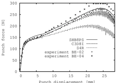
In order to validate the proposed solid–shell element, its predictions are compared to the experimental results of the NUMISHEET 2002 benchmarks. Two elements from the element library of the Abaqus code are also used in the comparison: the shell element S4R and the 3D continuum element C3D8I. Again, 150 uniformly distributed elements are used in the length direction for these two elements. However, two layers of C3D8I elements are required in the thickness direction in order to represent the stress distribution due to bending with sufficient accuracy. Also, ten C3D8I elements are used along the width direction in order to keep their aspect ratio in acceptable limits. Fig.4 displays the punch force versus punch displacement curves predicted by the three elements, along with the experimental results (BE-1,…, BE-4) from Meinders et al. [11].
Fig.4 shows that the numerical results obtained with SHB8PS element are the closest to the experimental results and they lay close to the solid element predictions. The slight differences between the two may be due to the different number and distribution of integration points along the thickness direction. The S4R element has too soft behavior with respect to SHB8PS and C3D8I elements.
The springback angles are also investigated, as they were also experimentally measured [11]. The springback phenomenon is particularly exacerbated in this unconstrained bending application, as illustrated in Fig.5. Table 2 summarizes the opening angles before and after springback for elements SHB8PS, C3D8I and S4R, compared to experiments. The simulated values with SHB8PS and C3D8I elements are close to each other and the closest to experiments. Comparing the numerical results to the experimental ones, the good performance of the SHB8PS solid– shell element is confirmed.
TABLE 2. Measured and simulated opening angles before and after springback.
Experimental Simulated
BE-01 BE-02 BE-03 BE-04 SHB8PS C3D8I S4R forming 22.7707 22.0064 23.0255 20.8599 23.0692 22.5820 33.3078 Springback 37.4212 35.6787 30.9036 35.3636 36.3952 32.0832 43.9071
FIGURE 4. Punch force vs. punch displacement plots for High Strength Steel
FIGURE 5. Deformed shape of the sheet in the unconstrained bending problem.
ACKNOWLEDGMENTS
The authors are grateful to the Agence Nationale de la Recherche–ANR (France) for its financial support through the Mat&Pro project FORMEF. The first author is grateful to the Region Lorraine for its financial support.
REFERENCES
1. F. Abed-Meraim and A. Combescure, International Journal for Numerical Methods in Engineering, 80, 1640-1686 (2009). 2. A. Legay and A. Combescure, International Journal for Numerical Methods in Engineering, 57, 1299-1322 (2003).
3. R.J. Alves de Sousa, R.P.R. Cardoso, R.A. Fontes Valente, J.W. Yoon, J.J. Grácio and R.M. Natal Jorge, International Journal for Numerical Methods in Engineering, 67, 160–188 (2006).
4. S. Reese, Computer Methods in Applied Mechanics and Engineering, 194, 4685–4715 (2005).
5. O. Zienkiewicz, R. Taylor and J. Too, International Journal for Numerical Methods in Engineering, 3, 275–290 (1971). 6. T. Hughes, M. Cohen and M. Haroun, Nuclear Engineering Design, 46, 203–222 (1978).
7. J. Simo and M. Rifai, International Journal for Numerical Methods in Engineering, 29, 1595–1638 (1990). 8. T. Belytschko and L. Bindeman, Computer Methods in Applied Mechanics and Engineering, 105, 225–260 (1993).
9. J. Hallquist, "Theoretical manual for DYNA3D". Tech. Rep. Report UC1D-19401, Lawrence Livermore National Laboratory, Livermore, CA, 1983.
10. D. Flanagan and T. Belytschko, International Journal for Numerical Methods in Engineering, 17, 679–706 (1981).
11. T. Meinders, A. Konter, S. Meijers, E. Atzema and H. Kappert, "A sensitivity analysis on the springback behavior of the unconstrained bending problem. In:NUMISHEET 2005, 6th international conference and workshop on numerical simulation of 3D sheet metal forming processes. Detroit, Michigan, USA, 2005.