HAL Id: hal-01164695
https://hal-ensta-paris.archives-ouvertes.fr//hal-01164695
Submitted on 17 Jun 2015HAL is a multi-disciplinary open access
archive for the deposit and dissemination of sci-entific research documents, whether they are pub-lished or not. The documents may come from teaching and research institutions in France or abroad, or from public or private research centers.
L’archive ouverte pluridisciplinaire HAL, est destinée au dépôt et à la diffusion de documents scientifiques de niveau recherche, publiés ou non, émanant des établissements d’enseignement et de recherche français ou étrangers, des laboratoires publics ou privés.
Statistics and dynamics of the boundary layer
reattachments during the drag crisis transitions of a
circular cylinder
Olivier Cadot, A Desai, S Mittal, S Saxena, B Chandra
To cite this version:
Olivier Cadot, A Desai, S Mittal, S Saxena, B Chandra. Statistics and dynamics of the boundary layer reattachments during the drag crisis transitions of a circular cylinder. Physics of Fluids, American Institute of Physics, 2015, 27, pp.014101. �10.1063/1.4904756�. �hal-01164695�
AIP/123-QED
Statistics and dynamics of the boundary layer reattachments during the drag crisis transitions of a circular cylinder
O. Cadot,1, a) A. Desai,2, 3 S. Mittal,2, 3 S. Saxena,2 and B. Chandra2
1)Unit´e de M´ecanique, Ecole Nationale Sup´erieure de Techniques Avanc´ees,
ParisTech, 828 Boulevard des Mar´echaux, 91762 Palaiseau Cedex, France
2)National Wind Tunnel Facility, Indian Institute of Technology Kanpur,
UP 208 016, India
3)Department of Aerospace Engineering, Indian Institute of Technology Kanpur,
UP 208 016, India (Dated: 5 December 2014)
Time series of pressure measured on the periphery of the central section of a circular cylinder of aspect ratio 22 are used to investigate the dynamics of the local reattach-ments during the drag crisis transitions. A succession of multi-stable dynamics are identified and characterized through conditional statistical analysis as the Reynolds number is increased. The first transition marking an abrupt weakening of the peri-odic pressure fluctuations associated to the global shedding dynamics is accompanied by the appearance of symmetric and bistable perturbations. Afterwards, two scenarii of asymmetric and symmetric boundary layer reattachments are found. The asym-metric scenario leads to two transitions. During the first transition the flow explores randomly three stable states to eventually stabilizes on the state corresponding to the permanent reattachment on one side of the cylinder. The second transition is bistable and leads to the permanent reattachment on both sides. For the second symmetric scenario, the boundary layer reattachments occur simultaneously on both side of the cylinder. In that case, the flow explores randomly two stable states to eventually stabilizes on the state of full reattachment. Pressure distributions of all of these states are characterized as well as their corresponding probabilities during the drag crisis transitions of the critical regime.
PACS numbers: 47.20.Ky,47.27.Cn,47.27.wb
Keywords: drag crisis, multi-stability, turbulent transition.
I. INTRODUCTION
Boundary layer reattachment behind a cylinder placed in a uniform velocity field is one of the most spectacular feature in fluid mechanics that can be observed when the Reynolds number is increased. Due to the substantial drag reduction it causes, this effect called ”drag crisis” has naturally motivated a lot of interest for many researches and applications in aeronautics. Pioneering measurements dating from the beginning of the last century (see for instance Wieselsberger1, Fage2) are reported by Roshko3 who compiled previous data
of mean drag, base pressure coefficient and Strouhal number for 104 < Re < 107. These works, and many others, later allowed the establishment of different flow regimes that can be found in the book of Zdravkovich4. These flow regimes are referred to as subcritical Re < 105, critical 105 < Re < 5× 10⁵, supercritical 5× 10⁵ < Re < 5× 10⁶ to transcritical
Re > 5× 10⁶. In the critical Reynolds number regime, the boundary layer transition from
laminar to turbulent flow is accompanied by the occurrence of asymmetric flow states5,6 producing a non zero mean lift. They are commonly called one bubble and two bubbles transitions corresponding respectively to the reattachment on one side and both sides of the cylinder. Although experiments of different origin always report transitions in roughly the same range of Reynolds numbers, the discrepancies in the comparison of, for example, the mean drag curves7 evidences the sensitivity of the phenomenon with the flow condition and cylinder’s surface preparation. The influence of the free stream turbulence was character-ized by Fage and Warsap8, Norberg and Sund´en9, Blackburn and Melbourne10 and many
studies6,8,11–13 were devoted to the surface roughness effect on the drag crisis. Nonetheless, the characterization of the different states are now well established (see Zdravkovich4).
On the other hand, the dynamics and the nature of the fluctuations associated with these transitions still needs some investigations. Most of the studies about fluctuations during the drag crisis focus on the global K´arm´an mode5,14, and especially the measurement of the Strouhal frequency. Consequently, the dynamics of the transitions between the one bubble and two bubbles states is less studied than the weakening of the shedding. From global force11,15 and local pressure7 measurements, the existence of bistable behaviors in the
criti-cal range has been evidenced through hysteretic discontinuities in the Strouhal - Reynolds number relationship. Schewe15 associated each discontinuity to a subcritical bifurcation during which the energy of the force fluctuations is dominated by the contribution of a wide
low frequency domain7,11,15. This domain belongs to lower frequencies than the nearly
ex-tinguished frequencies of the K´arm´an global modes. Recently Miau et al.16 and Lin et al.17
studied the pressure time series measured on the cylinder and noted that reattachments might switch from one side to the other during the fluctuations as previously observed by Farell and Blessmann7. Furthermore, the presence of reattachment on one side or on the
other was unpredictable in time. The characteristic time of the switch is much larger than the periodic shedding, thus questioning the accuracy of results obtained by time averaging.
An interesting aspect relates to the three dimensionality of the flow reattachments along the span of the cylinder. Although its experimental investigation18,19 is a hard task, it is
now generally agreed that the reattachment process is not a two dimensional phenomenon but involves sub-domains17,20 along the span in which the above scenario takes place. There
is then a succession of local transitions that leads to the global drag crisis. The question on how these sub-domains interact remains an open issue.
From a numerical point of view, the full resolution of the transitions in drag crisis via solution to Navier Stokes equations remains a challenge. Singh and Mittal21 carried out
a simulation of the two-dimensional Navier Stokes equation. They were able to reproduce the general phenomenon of drag crisis through their 2D simulations. More recently, Behara and Mittal22 performed a large eddy simulation (LES) of the 3D flow using a Smagorinsky
model. They also computed the flow in the presence of a roughness element that simulates a trip wire placed at θ = 55◦ from the front stagnation point of the cylinder, with respect to the free-stream direction. It was shown that for the clean cylinder, without any roughness element, the time-averaged flow is symmetric for all situations and the time-averaged lift coefficient remains close to zero during the drag crisis transitions. However, in the presence of the roughness element, that simulates a possible geometric defect in the symmetry of the set-up, the numerical simulation is able to retrieve the asymmetric states that are commonly observed in experiments. Based on the results from their simulations, Behara and Mittal22 proposed a hypothesis for the chain of events during the transitions related to drag crisis. A more recent effort of 3D LES simulation due to Rodriguez et al.23 also succeeded to retrieve
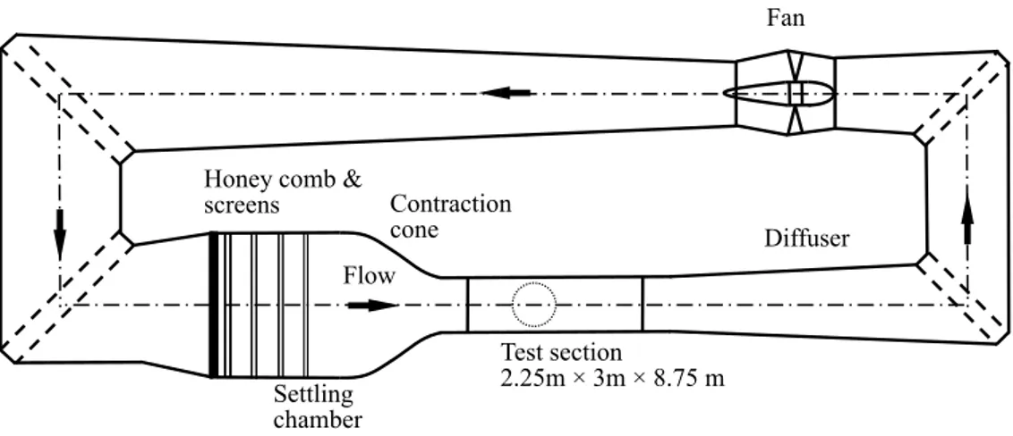
Contraction Honey comb &
screens cone Flow Settling chamber Fan n Diffuser Test section 2.25m × 3m × 8.75 m
FIG. 1. Aerodynamic layout of the National Wind Tunnel Facility (NWTF).
The goal of our work is to investigate the dynamics of the flow reattachment inside one of the sub-domains. We then focus on the boundary layers states in the central cross section of the cylinder and explore slight variations of the Reynolds number around the transi-tions. Long time recordings are performed in order to display the corresponding statistics. The details of the experimental set-up are described in Section II. In subsection II A we first present the details of the wind-tunnel. The flow geometry along with the pressure measurements are presented in subsection II B. The results are presented in section III. This section has four parts. Part III A evidences the flow transitions for two experiments presenting different scenarii: the asymmetric and symmetric scenario. Part III B is de-voted to the weakening of the periodic fluctuations in the vicinity of the cylinder that is observed in the same manner for both experiments. Subsections III C and III D present the statistics and the dynamics of the reattachment during the asymmetric and the symmet-ric scenario respectively. Finally, discussions and conclusions are presented in the section IV.
II. EXPERIMENT
A. National Wind Tunnel Facility
The facility is a closed-circuit, continuous, atmospheric, low-speed wind tunnel. The layout is shown in Fig. 1. The cross section of the test area is 3 m×2.25 m with a total length
of 8.75 m. It is equipped with two turntables (indicated as dashed circle in Fig. 1), one on the upper surface facing the other one in the lower surface. They can rotate synchronously. The cylinder is fixed at the centre of the turntables, say 3.5 m downstream the beginning of the test section. Upstream of this test section, the tunnel has a wide area contraction ratio 9 : 1. The maximum air speed is 80 m.s−1, which is produced by a single stage 12-bladed axial flow fan powered by a 1000 kW variable speed DC motor. It has four anti-turbulence screens placed downstream of the honeycomb which ensure a low turbulence intensity. The spatial inhomogeneities of the incoming flow are estimated through measurements of the vertical velocity profile obtained by means of a pitot tubes rack placed at the centre of the turntables. Figure 2(a) shows two vertical profiles non dimensionalized as 100∗ u(z)−UU where U in the mean wind speed used to compute the flow Reynolds number. We can see that the inhomogeneity is the largest for the lower velocity, but still remains very low. Actually, the root mean square value of the z-velocity profiles supplies an estimation of a global spatial inhomogeneity as TH =
√
<(u(z)−U)2>
U , where < .. > denotes an averaging
over all the measured velocities u(z) along the z-direction. In the worst case obtained for the lowest wind speed of U = 20 m.s−1, TH = 0.05% and decreases to TH = 0.025% for U = 60 m.s−1. The boundary layer velocity profiles have been measured at the centre of the turntables by means of a pitot tubes rack. The boundary layers thickness is fairly constant in the investigated range of velocities and worth δ99∼= 96 mm.
The turbulence intensity TU is estimated from single hot wire measurements at
mid-height. It is defined as the root mean square value of the measured velocity fluctuations time series divided by the mean. To compute the fluctuating part of the velocity signal, a cut off of 3 kHz for the low pass filter and 10 Hz for the high pass filter is used. We obtain TU ∼ 0.05% as shown in Fig. 2(b). When the low pass filtering is 10 kHz, and no high pass
filtering is used, the measured turbulence intensity is increased by a factor 2 and TU ∼ 0.1%
in the explored range. In addition, for reasons of completeness and possible repetitions of similar experiments in other facilities, Fig. 3 provides the rms fluctuations of the pressure at the front head of the test cylinder (as defined in section II B, Fig. 4). The measurements are reported for two different pressure scanners, the one used all through the present work described in section II B having a full scale range of ±5 kPa (with a resolution of ±2 Pa) and another one having a smaller range of ±1 kPa and a better accuracy of ±0.5 Pa. For low noise wind tunnel, the fluctuating pressure coefficient is known to be close to twice the
−0.50 −0.25 0 0.25 0.5 0.5 1 1.5 2 (u(z)−U)/U (%) z(m) 60 m.s−1 20m.s−1 (a) 20 30 40 50 60 0 0.02 0.04 0.06 0.08 0.1 U (m.s−1) (%) T U T H (b)
FIG. 2. Vertical mean velocity profiles in the test area for wind speeds of U = 60 m.s−1 and
U = 20 m.s−1 (a). Turbulent intensity at mid height TU and flow homogeneity TH measured from
the vertical mean velocity profiles (b).
turbulent intensity (see Surry24, Bruun and Davies25, Norberg26). The expected value of the fluctuating pressure coefficient at the stagnation point of the cylinder should then be about 0.1% on the basis of the turbulent intensity from velocity measurements. Even for the more accurate pressure scanner, the value of 2.5% obtained at low velocities in Fig. 3 exceeds this prediction very significantly. The discrepancy is ascribed to some background noise explained by the fact that the tunnel does not have anechoic treatments. For larger velocities, the pressure coefficient fluctuations fall below 0.8%. In the case of the wide range pressure scanner, it can be seen a large fluctuating pressure level of about 20 Pa on the whole range of the explored velocities that increases significantly the pressure coefficient fluctuations. The origin of the this large fluctuation is an electromagnetic noise, discovered after the data of the present article were obtained. This noise has not been filtered in the following since it only affects the pressure fluctuations in the vicinity of the stagnation point where the fluctuations are the lowest. Except in this region, the fluctuations are much larger than 0.1 (see Fig. 6b) and the electromagnetic noise that contribute by no more than 0.06 in the pressure fluctuation coefficient becomes negligible.
The temperature of the tunnel is not controlled. However, measurements are done when heating due to the fan is compensated by the thermal losses. In that case, the air tem-perature remains constant, and can take a value between 30◦C and 45◦C depending on the
20 30 40 50 60 0 0.02 0.04 0.06 0.08 0.1 U (m.s−1) Cp , (θ = 0 0 ) 20 30 40 50 60 0 10 20 30 U (m.s−1) p , (θ = 0 0 ) (Pa)
FIG. 3. Fluctuating pressure coefficient Cp′ as defined in Eq. 1 at the front head of the cylinder (θ = 0o) as described in Fig. 4 vs. the velocity in the wind tunnel. Empty symbols refer to the wide range pressure scanner which is used to obtain the result of the present work (section II B) and filled symbols correspond to a more accurate pressure scanner but having a smaller range. The inserted graphics display the corresponding pressure.
outdoor temperature. The kinematic viscosity of the air is thus simply corrected with the air temperature and static pressure in the wind tunnel to compute the Reynolds number of the flow.
B. Geometry and pressure measurements
The cylinder has a diameter d = 10 cm and a length L = 2.25 m. The Reynolds number of the flow Re = U dν is varied in the range 1.2× 10⁵ and 3.8× 10⁵. The cylinder is made out of aluminium in only one piece. It has been machined on its whole length after the holes for pressure measurements have been drilled. Thereafter, it is polished to obtain surface with a smooth finish. The relative roughness is estimated as k/d < 10−5, where k is the particle size of the polishing mixture. The cylinder can be considered smooth as per the classification due to Achenbach and Heinecke6. However, in the present study it has to be kept in mind that the pressure holes are introducing singular surface roughness that is much larger that the polished surface. Except these holes, residual geometric defects of the cylinder are no more than 0.1% of its diameter d for either the diameter variation at the mid section or along the exposed span of the cylinder. The cylinder is placed vertically in
the wind tunnel, flush mounted at the centre of the top and bottom turntables (the centre of the dashed circle in Fig. 1). During the experiments, no vibrations of the cylinder have been noticed. There are 30 pressure ports on the periphery of the cylinder at a section at the mid span to measure p(θ) as sketched in Fig. 4. The turntables allow the change of the angle of attack of the cylinder. The origin of the angular coordinate θ is always taken at the center of the front side of the cylinder whatever the angle of attack of the cylinder is. The static pressure p0 measured at the entrance of the test section is used to compute the
pressure coefficient as follows :
cp(θ, t) =
p(θ, t)− p0 1
2ρU2
(1) The pressure ports are connected via flexible tubes to a pressure scanner (model ESP 32HD) that acquires data at each port at a sampling frequency of 500 Hz. The measurements are naturally low pass filtered due to the tubing and the design of pressure probe. The resolution of pressure scanner is ±2 Pa. The estimated uncertainty on cp is of the order
of 0.01. The corresponding cut off frequency has been evaluated to be fc = 150 Hz on the
basis of the spectral analysis of pressure time series (not shown here) that display a strong cut-off frequency at this value irrespective to the main velocity U . The consequence is that our dynamic pressure measurements are limited to non dimensional frequencies lower than St = fcdU , or equivalently to St = 0.75 at the lowest velocity U = 20 m.s−1 and St = 0.25 at the larger explored wind speed. The periodic K´arm´an shedding dynamics observed around St = 0.2 is then resolved. On the other hand, the effect of frequency doubling5 associated
with the two bubbles transition is not. The pressure range of the scanner is limited to, approximately, -7000 Pa. This, unfortunately, limits our investigation to U ≤ 65 m.s−1. The corresponding saturated values of cp will be indicated on the relevant plots. For a given
mean flow velocity, the pressure time series are recorded for a duration of 120 s. To explore the effect of the Reynolds number on the flow transitions, measurements have always been performed by increasing the wind velocity. For any quantity a, A denotes the time averaged value and A′ the standard deviation.
The sectional form drag cD and lift cL coefficients are computed as : cD(t) = 1 2 I cp(θ, t)cos(θ)dθ cL(t) = 1 2 I cp(θ, t)sin(θ)dθ. (2)
FIG. 4. Central section of the cylinder. Each tick symbolizes a hole of 1 mm dedicated for wall pressure measurements. The side 0◦ < θ < 180◦ will be referred as the top side in the text, the side 180◦ < θ < 360◦ as the bottom side.
The times series are utilized to calculate the time-averages CD, CL and standard deviations CD′ , CL′ . The force coefficient in Eq. 2 are calculated with a trapezoidal integration of the angular distribution cp(θ). The absolute uncertainty in the force coefficients is estimated to
be about ±0.02.
Eventually, to characterize the symmetry of the flow we measured the mean pressure distributions for two cases of angle of attack of the cylinders (that will be studied in the following) for the subcritical regime at Re = 1.85× 10⁵. We can observe in Fig.5 a slight defect of symmetry. Since this asymmetry is identical for angle of attacks, we conclude that the cylinder is not the cause but rather the lateral main flow inhomogeneity (’lateral’ refers to the direction perpendicular to the incoming flow in the mid-span cross sectional plane). In addition, we can see very little difference in the pressure coefficient level around θ = 60◦ between the two angles of attack. This small difference remains close to the experimental uncertainties.
III. RESULTS
A. Transitions
Fig. 6(a) shows the mean pressure coefficient Cp(θ, Re). This figure identifies the Reynolds
number for which reattachments of the flow occur on the central section of the cylinder. In the subcritical regime , the pressure coefficient is typically27 equal to−1 near the separation region on the cylinder (θ ∼ 80◦). However, after the reattachment of the boundary layer
0 60 120 180 240 300 360 −1.5 −1 −0.5 0 0.5 1 θ (°) C p 0 60 120 180 240 300 360 −1.5 −1 −0.5 0 0.5 1 θ (°) C p AoA=0° AoA=84°
FIG. 5. Comparison of the angular distribution of the pressure coefficient for the subcritical regime at Re = 1.85× 10⁵ obtained for both angles of attack 0◦ and 84◦ of the cylinder.
the pressure coefficient decreases below −2.5 in the same region. The first reattachment is observed around Re = 3.3× 10⁵ on the top side of the cylinder (as defined in Fig. 4) and then the second reattachment at about Re = 3.6× 10⁵ on its bottom side. Same effects on
the pressure distribution can be found in Raeesi, Cheng, and Ting20; this is the scenario of
successive reattachments which are referred to as one bubble and the two bubbles transition (see Zdravkovich4). The variation of the fluctuation of the pressure coefficient, C′
p, with Re
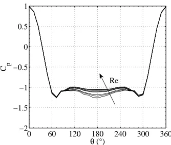
and θ is shown in Fig. 6(b). Cp′ increases significantly before each reattachment in the zone of separation (between 60◦ and 120◦ on the top side and 240◦ and 300◦ on the bottom side). For lower Re, the fluctuation globally decreases gradually from Re = 105 to Re = 2.5× 10⁵.
Figure 7 shows another experiment but for which the cylinder has been rotated by an angle of 84◦. The sensitivity of the drag crisis11 to geometrical defects is then evidenced since
the scenario of reattachments is now quite different. Drastic changes after a rotation of the cylinder was also reported by Batham28. The interesting feature in our case is the appearance of a simultaneous reattachment on both sides of the cylinder (two bubbles tran-sition) around Re = 3.6× 10⁵ as observed in Fig. 7(a). Such a symmetric scenario has also been observed by Norberg and Sund´en9 for a free stream turbulence intensity of 1.4%. As
noted in the previous scenario case, reattachments are preceded by significant increase in fluctuations around the separation region. This is seen clearly in Fig. 7(b).
1.25 1.5 1.75 2 2.25 2.5 2.75 3 3.25 3.5 3.75 x 10⁵ 0 60 120 180 240 300 360 Re θ (°) (a) Cp −3 −2 −1 0 1 1.25 1.5 1.75 2 2.25 2.5 2.75 3 3.25 3.5 3.75 x 10⁵ 0 60 120 180 240 300 360 Re θ (°) (b) Cp’ 0 0.2 0.4 0.6 0.8
FIG. 6. Mean (a) and rms value (b) of the angular distribution of the pressure coefficient vs. Re. In (a) the exterior iso-Cp line is 0.8 with intervals of 0.2. In (b) the exterior iso-Cp′ line is 0.1 with
intervals of 0.1.
The consequences on the sectional drag and lift of these pressure distributions are dis-played in Fig. 8 and 9 for the two observed scenario. Both cases, in Fig. 8(a) and 9(a), lead to the same reduction in drag and achieve CD = 0.6 at Re = 3.8× 10⁵. The lift
fluctua-tion in Fig. 8(b) and 9(b) indicates a very sharp transifluctua-tion common to both experiments at Re = 2.6× 10⁵. For Reynolds numbers lower than 2.6× 10⁵, both drag and lift coefficients
evolution are comparable for both scenarii. It should be mentioned that the lift coefficient of the second scenario (Fig. 9b) is lower than that of the first one (Fig. 8b). This is due to the slight difference in the pressure distribution measured for both angles of attack as
1.25 1.5 1.75 2 2.25 2.5 2.75 3 3.25 3.5 3.75 x 10⁵ 0 60 120 180 240 300 360 Re θ (°) (a) Cp −3 −2 −1 0 1 1.25 1.5 1.75 2 2.25 2.5 2.75 3 3.25 3.5 3.75 x 10⁵ 0 60 120 180 240 300 360 Re θ (°) (b) Cp’ 0 0.2 0.4 0.6 0.8
FIG. 7. Mean (a) and rms value (b) of the angular distribution of the pressure coefficient vs. Re. The only difference with the experiment in Fig. 6 is that the cylinder has been rotated by an angle of 84◦.
displayed in Fig. 5 and related to experimental uncertainties as mentioned in section II B. For larger Reynolds numbers in Fig. 8(b), the one bubble transition is associated with a strong positive lift production and the two bubbles transition to a small negative lift. How-ever, we do not reach a sufficiently high Reynolds number to observe a return to symmetric flow with zero lift (supercritical regime). In the case of symmetric reattachment scenario in Fig. 9(b), only a small negative lift is observed because the one bubble transition has been bypassed.
1.25 1.5 1.75 2 2.25 2.5 2.75 3 3.25 3.5 3.75 x 10⁵ 0 0.2 0.4 0.6 0.8 1 1.2 1.4 Re (a) C D C D’ 1.25 1.5 1.75 2 2.25 2.5 2.75 3 3.25 3.5 3.75 x 10⁵ 0 0.2 0.4 0.6 0.8 1 1.2 1.4 Re (a) C D C D’ 1.25 1.5 1.75 2 2.25 2.5 2.75 3 3.25 3.5 3.75 x 10⁵ −0.2 0 0.2 0.4 0.6 0.8 1 Re (b) C L C L’ 1.25 1.5 1.75 2 2.25 2.5 2.75 3 3.25 3.5 3.75 x 10⁵ −0.2 0 0.2 0.4 0.6 0.8 1 Re (b) C L C L’
FIG. 8. Sectional mean and fluctuations drag and lift vs. Re computed from the data of the asymmetric reattachments in Fig. 6.
2.6 × 10⁵. This is followed by a study of the two different reattachment scenarii: the
asymmetric and symmetric reattachments.
B. Weakening of the shedding activity
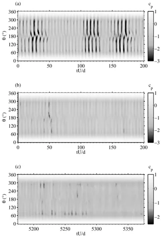
The periodic pattern observed in the space-time diagrams cp(θ, t) in Fig. 10 indicates
alternate vortex shedding. As can be seen from the periodic pressure variation, the activity at Re = 1.22× 10⁵ (Fig. 10a) is more intense than at Re = 2.45× 10⁵ (Fig. 10b). This is
made clearer in Fig. 11, by looking at the corresponding time series of the lift coefficient. This attenuation is the cause of the continuous reduction of the lift fluctuations observed for Re < 2.5× 10⁵ in Figs. 8(b) and 9(b). In this range of Re, it is noteworthy that the
1.25 1.5 1.75 2 2.25 2.5 2.75 3 3.25 3.5 3.75 x 10⁵ 0 0.2 0.4 0.6 0.8 1 1.2 1.4 Re (a) C D C D’ 1.25 1.5 1.75 2 2.25 2.5 2.75 3 3.25 3.5 3.75 x 10⁵ −0.2 0 0.2 0.4 0.6 0.8 1 Re (b) C L C L’
FIG. 9. Sectional mean and fluctuations drag and lift vs. Re computed from the data of the symmetric reattachments in Fig. 7.
pressure distribution upstream of the separation remains unaltered as shown in Fig. 10(c). As the shedding gets weaker the base pressure rises. This correlation can be observed in the space-time diagram in Fig. 10(a) where, on an average, the base pressure is larger when the vortex shedding activity is less intense. As a consequence, the corresponding drag is lower during low intensity shedding as can be seen in Fig. 11(a).
At Re = 2.56× 10⁵, a new feature characterized by durations of absence of periodic fluc-tuations appears. An abrupt end of the vortex shedding activity seen by the pressure taps is observed at tU/d ≃ 5300 in the space-time diagram in Fig. 10(c) and in the corresponding lift coefficient in Fig. 11(c). It is even better quantified in Fig. 13 which shows the same time series but for the pressure coefficients at θ = 60◦ and 300◦ only and for a very long time
0 50 100 150 200 0 60 120 180 240 300 360 tU/d θ (°) (a) cp −3 −2 −1 0 1 0 50 100 150 200 0 60 120 180 240 300 360 tU/d θ (°) (b) c p −3 −2 −1 0 1 5200 5250 5300 5350 0 60 120 180 240 300 360 tU/d θ (°) (c) c p −2 −1 0 1
FIG. 10. Space time diagrams of the pressure distribution cp(θ, tU/d) for (a) Re = 1.22× 10⁵, (b)
Re = 2.45× 10⁵ and (c) Re = 2.56× 10⁵.
duration (tU/d = 104). The flow switches between high fluctuations due to intense shedding,
and low fluctuations with weak shedding related activity. The time duration between these switches is about 2 or 3 order of magnitudes larger than the time period of vortex shedding (a periodicity of tU/d ∼ 5 is observed in Fig. 11 when tU/d < 5300). It is clear from Fig. 13(a) that this long time dynamics is associated with symmetric perturbations since the low pass filtered time series extracted from the two symmetric angular positions ±60◦ are in phase.
The probability density functions of the low pass filtered pressure time histories of cp(60◦, t)
(Fig. 13b) and cp(300◦, t) (Fig. 13c) display a discontinuity when Re is increased. In the
regime Re = 2.56 ∼ 2.58 × 10⁵, there are two most probable values for the pressure
coef-ficient. This shows that the flow is a combination of two states. Subsequent to this first transition for Re > 2.6× 10⁵, the pressure distribution shown in Fig. 6 and Fig. 7 is little
0 50 100 150 200 −2 −1 0 1 2 tU/d c L , c D (a) 0 50 100 150 200 −2 −1 0 1 2 tU/d c L , c D (b) 5200 5250 5300 5350 −2 −1 0 1 2 tU/d c L , c D (c)
FIG. 11. Drag, cD (thick line) and lift, cL (thin line) coefficients corresponding to Fig. 10 for (a)
Re = 1.22× 10⁵, (b) Re = 2.45× 10⁵ and (c) Re = 2.56× 10⁵. 0 60 120 180 240 300 360 −2 −1.5 −1 −0.5 0 0.5 1 θ (°) C p Re
FIG. 12. Mean pressure distribution Cp(θ) for 1.22× 10⁵< Re < 2.56× 10⁵. The arrow indicates
0 0.5 1 1.5 2 2.5 3 3.5 4 x 10⁴ −2 −1.5 −1 −0.5 0 0.5 tU/d cp (60°), c p (300°) (a) 2.2 2.3 2.4 2.5 2.6 2.7 x 10⁵ −1.3 −1.2 −1.1 −1 Re (b) c p (60 ° ) 2.2 2.3 2.4 2.5 2.6 2.7 x 10⁵ −1.3 −1.2 −1.1 −1 Re (c) c p (300 ° )
FIG. 13. Signals with large fluctuations in (a) are the time series for the two symmetric angular positions cp(60◦, tU/d) (bottom) and cp(300◦, tU/d) (top) at Re = 2.56×10⁵. For clarity, cp(300◦, t)
is artificially shifted by 1. Thin lines are the low pass filtered time series. Probability functions of the filtered time series of pressure (b) cp(60◦) and (c) cp(300◦) vs. Re.
affected by Re until reattachments appear around Re = 3.3× 10⁵ for the asymmetric sce-nario and Re = 3.6× 10⁵ for the symmetric scenario.
In summary, there is a gradual reduction of the pressure fluctuations on the cylinder that is due to a weakening of the periodic shedding with Re. This is followed by an abrupt reduction in CL′ due to a transition to a bistable state. In a more quantitative manner, it is useful to use the joint probability density function of the pressure coefficients measured at two symmetrical angles as introduced by Norberg26. In our case, we chose θ =±84◦ (we note that θ = −84◦ corresponds to θ = 276◦). At these angular locations the pressure is very sensitive to the periodic shedding and reattachment process. The statistical analysis is performed on the entire acquisition of 120 s of the pressure time series. The joint PDFs are shown in Fig. 14 for three typical Reynolds numbers that are characteristic of the flow prior to the reattachments. The antisymmetric coherent periodic shedding activity at Re = 1.22 × 10⁵ in Fig. 14(a) is revealed by the -1 slope correlation26. The very significant
c p(84°) c p (276°) (a) −3.5 −2.5 −1.5 −0.5 0.5 −3.5 −3 −2.5 −2 −1.5 −1 −0.5 0 0.5 c p(84°) c p (276°) (b) −3.5 −3 −2.5 −2 −1.5 −1 −0.5 −3.5 −3 −2.5 −2 −1.5 −1 −0.5 cp(84°) c p (276°) (c) −3.5 −3 −2.5 −2 −1.5 −1 −0.5 −3.5 −3 −2.5 −2 −1.5 −1 −0.5
FIG. 14. Joint probability density function of cp(84◦) and cp(276◦) for (a) Re = 1.22 105, (b)
Re = 2.59 105 and (c) Re = 2.99 105.
weakening of the periodic vortex shedding activity at Re = 2.59× 10⁵ leads to the absence
of any correlation in Fig. 14(b). For larger Re, and before the reattachment process, a small but significant tendency to a positive correlation of slope +1 is observed as shown in Fig. 14(c) for Re = 2.99× 10⁵. Then, after the abrupt transition of the periodic lift
extinguishment observed around Re = 2.6 × 10⁵, the flow dynamics undergoes coherent
symmetric perturbations. Next, we study the dynamics in the asymmetric reattachments scenario.
C. Asymmetric reattachments
An overview of the experiment associated with asymmetric reattachments is presented in Fig. 6. Space-time diagrams of the pressure distribution for a duration of tU/d = 2000, at different stages of the reattachments, are shown in Fig. 15. The symmetric perturbations presented above are clearly observable in Fig. 15(a) for Re = 2.99× 10⁵. They correspond
to the light vertical stripes affecting the whole pressure distribution and with typical time durations of tU/d ∼ 100. The intermittent appearance of low pressure (as dark patches)
in Fig. 15(b) at Re = 3.37× 10⁵ on either side of the cylinder is associated with boundary
layer reattachment. At Re = 3.49× 10⁵, only the reattachment on the top side remains
permanent in Fig. 15(c). In Fig. 15(d), the reattachment on the bottom side appears inter-mittently. Finally, full reattachment on both sides of the cylinder is observed in Fig. 15(e) at Re = 3.78× 10⁵.
Correspondingly, the joint PDFs of the pressure coefficients measured at θ = 84◦ and 276◦ are presented in Fig. 16. During the reattachment process from Re = 2.99× 10⁵ to Re = 3.78×10⁵, the joint PDFs evidence four most probable states via existence of four local
maxima. These states belong to each quadrant defined by the two frontiers cp(84◦) =−2 and cp(276◦) =−2 and denoted by #0, #1b, #1t and #2 in Fig. 16(a). The state #0 is ascribed
to no reattachment. The states #1b and #1t are ascribed to bottom side reattachment only and top side reattachment only, respectively. The state #2 corresponds to full reattachment on both sides of the cylinder. States #1b and #1t might be called one bubble states and #2, the two bubbles state. From Fig. 16(a), we can see that the flow explores the three states #0, #1b, #1t with different probabilities. By increasing the Reynolds number, only the reattachment on the top is present (state #1t in Fig. 16(b)). Again, during the second reattachment in Fig. 16(c) both states #1t and #2 are present with different probabilities. Finally, only the state #2 prevails in Fig. 16(d) for the full reattachment.
The quantification of the proportion of states visited during the reattachment dynamics is carried out by plotting conditional statistics in the four quadrants as a function of the Reynolds number. We present the probability of each states estimated from the integral of the joint PDF in each quadrant. The proportion of states is plotted in Fig. 17 in a semi-log representation. Conditional statistics performed on the states also provide the associated pressure distribution. For the following analysis, we define the boundary layer separation location around the strong curvatures present on both sides of the base pressure plateau of the pressure distribution.
We first look at the primary reattachment that occurs on the top side of the cylinder in the Reynolds number range 3×10⁵ < Re < 3.45×10⁵. The pressure distributions corresponding
to the conditional statistics of state #0 are displayed in Fig.18(a). Whatever its proportion in Fig.17 during the reattachment dynamics, the distributions are fairly identical. This implies that there is no significant dependance on the Reynolds number. State #0 corresponds to a
0 500 1000 1500 2000 0 60 120 180 240 300 360 tU/d θ (°) (a) cp −3 −2 −1 0 1 0 500 1000 1500 2000 0 60 120 180 240 300 360 tU/d θ (°) (b) c p −3 −2 −1 0 1 0 500 1000 1500 2000 0 60 120 180 240 300 360 tU/d θ (°) (c) cp −3 −2 −1 0 1 0 500 1000 1500 2000 0 60 120 180 240 300 360 tU/d θ (°) (c) c p −3 −2 −1 0 1 0 500 1000 1500 2000 0 60 120 180 240 300 360 tU/d θ (°) (d) c p −3 −2 −1 0 1
FIG. 15. Space time diagrams of the pressure distribution cp(θ, tU/d) for (a) Re = 2.99× 10⁵, (b)
Re = 3.37× 10⁵, (c) Re = 3.49× 10⁵, (d) Re = 3.59× 10⁵ and (e) Re = 3.78× 10⁵.
separation located at around 96◦ that is delayed compared to the subcritical flow depicted in Fig. 12. Conditional pressure distribution describing state #1t is shown in Fig.18(b).
c p(84°) c p (276°) (a) −3.5 −3 −2.5 −2 −1.5 −1 −0.5 −3.5 −3 −2.5 −2 −1.5 −1 −0.5 #0 #1b #1t #2 c p(84°) c p (276°) (b) −3.5 −3 −2.5 −2 −1.5 −1 −0.5 −3.5 −3 −2.5 −2 −1.5 −1 −0.5 cp(84°) c p (276°) (c) −3.5 −3 −2.5 −2 −1.5 −1 −0.5 −3.5 −3 −2.5 −2 −1.5 −1 −0.5 cp(84°) c p (276°) (c) −3.5 −3 −2.5 −2 −1.5 −1 −0.5 −3.5 −3 −2.5 −2 −1.5 −1 −0.5
FIG. 16. Joint probability density function of cp(84◦) and cp(276◦) for (a) Re = 3.37× 10⁵, (b)
Re = 3.49× 10⁵, (c) Re = 3.59× 10⁵ and (d) Re = 3.78× 10⁵. Vertical and horizontal dashed lines
show the saturated value introduced by the higher limit of the pressure scanner.
All the pressure distributions indicate a separation around 120◦. This suggests that state #1t is a reattached boundary layer on the top side of the cylinder. A clear dependency with the Reynolds number is observed; as it is increased, the lowest pressure decreases and the separation location is displaced slightly beyond 120◦. On the other side of the cylinder, the separation is not affected and remains at the same location as for state #0. As already evidenced in the joint PDF (Fig. 16a), even if primarily the top side is reattaching, a few events of reattachment (less that 1.5%) on the bottom side are also observed at Re = 3.3× 10⁵. The pressure distribution corresponding to the conditional statistics of
state #1b in Fig. 18(c) proves the existence of the reattachment on the bottom side. The state #1b is the antisymmetric of state #1t.
We turn now to the second reattachment dynamics which is produced in the Reynolds number range 3.5 × 10⁵ < Re < 3.8 × 10⁵ on the bottom side of the cylinder. During
this transition the states #1t and #2 are the most probable states. The corresponding pressure distribution for the states are shown in Figs. 19(a) and 19(b), respectively. All the Cp curves superimpose satisfactorily on the top side (0 < θ < 180◦) in both figures
3 3.1 3.2 3.3 3.4 3.5 3.6 3.7 3.8 x 10⁵ 10−3 10−2 10−1 100 Re Conditional probability #0 #2 #1b #1t
FIG. 17. Probability of the conditional statistics of states #0, #1b, #1t and #2 during the asymmetric reattachment process.
meaning that the reattached flow does not depend on the Reynolds number for these states. The Cp distribution in the range 0◦ < θ < 180◦ is affected by the condition whether there
is a reattachment or not of the boundary layer on the bottom side (180◦ < θ < 360◦). In state #1t (Fig. 19a), the separation on the bottom side is located within the range 252◦ − 264◦ which is comparable to a non-reattached boundary layer. In this case, the permanently attached boundary layer, on the top side, produces a very low pressure with Cp around −2.8 at 84◦ as for Re = 3.45× 10⁵ in Fig. 18(b). For state #2, the separation
located in the range 228◦−240◦ indicates a reattachment. Correspondingly, the permanently attached boundary layer, on the top surface, produces a higher pressure with Cp around −2.6 at 84◦. It, therefore, appears that the second reattachment weakens the permanent
primary reattachment. It is worth noticing that in contrast to the first reattachment, the separation location during the second reattachment depends significantly on the Reynolds number and moves progressively from about 240◦ to 230◦, approximately (or from−120◦ to −130◦) as located by the dashed lines in Fig. 19(b). Despite the Reynolds number effect
observed on the bottom side, the state #1t describes one side reattachment, and state #2 full reattachment. A few events of detachments (less than 2%) on the top side are also observed around Re = 3.65× 10⁵ (see Fig. 17) and their pressure distributions are shown
in Fig. 19(c). These are the antisymmetric situation of the distributions of states #1t in Fig. 19(a).
0 60 120 180 240 300 360 −3 −2 −1 0 1 θ (°) C p (a) #0 0 60 120 180 240 300 360 −3 −2 −1 0 1 θ (°) C p (b) #1t 0 60 120 180 240 300 360 −3 −2 −1 0 1 θ (°) C p (c) #1b
FIG. 18. Pressure distributions of the conditional statistics #0 (a), #1t (b), #1b (c) for Reynolds numbers in the range 2.99× 10⁵ < Re < 3.45× 10⁵ during the primary reattachment of the antisymmetric scenario. Arrows are indicating the hierarchy of the curves for increasing Re.
To conclude this part on the asymmetric scenario, we show in Fig. 20, the pressure distributions of the states observed during the two lift fluctuation peaks observed in Fig. 8, at Re = 3.35× 10⁵ in Fig.20(a) and at Re = 3.59× 10⁵ in Fig.20(b). The fluctuations for
the first peak in CL′, are due to the dynamics of the nearly equal exploration of state #0 corresponding to no reattachment, and state #1t corresponding to the reattachment of the boundary layer on the top side of the cylinder only. Few events of state #1b representing 0.5% of the time spent corresponds to the reattachment on the bottom side only. It is noteworthy that while the proportion of states #1b and #1t differ by two order of magnitudes, they exhibit mirror symmetry with respect to each other. For the second peak, the fluctuations are due to the dynamics of exploration of three states: 62% of state #2 corresponding to full reattachment, 37% of state #1t corresponding to the reattachment of the boundary layer on the top side of the cylinder only and 1% of state #1b corresponding to the reattachment on the bottom side only. For both fluctuations, the reattachment dynamics is random as can be observed via the statistics of state changes. We consider the realization to be in a given state
0 60 120 180 240 300 360 −3 −2 −1 0 1 θ (°) C p (a) #1t 0 60 120 180 240 300 360 −3 −2 −1 0 1 θ (°) C p (b) #2 0 60 120 180 240 300 360 −3 −2 −1 0 1 θ (°) C p (c) #1b
FIG. 19. Pressure distributions of the conditional statistics #1t (a), #2 (b), #1b (c) for Reynolds numbers in the range 3.5 × 10⁵ < Re < 3.8 × 10⁵ during the secondary reattachment of the antisymmetric scenario. Arrows are indicating the hierarchy of the curves for increasing Re. Dashed lines help to locate the separation angles.
in a time interval dt = 1/fs, where fs = 500Hz is the sampling frequency of the pressure
time series recording. Let us call k, the number of consecutive realizations giving the same state considered as a random variable. Hence kdt represents the time lapse between two consecutive state changes. Practically, the time lapse is measured from the duration between two consecutive pressure coefficient of level -2 in the time series of cp(θ = 84◦, t). In order
to obtain better statistical convergence, a long time series (380s) has been recorded for the case Re = 3.35×10⁵ only. In that case, the total signal duration is 2.09×10⁵ d
U and the time
interval during which the realization is to be in a given state, is dt = 1.1Ud. The resulting experimental probability P (k) shown in Fig. 21 (empty circles) displays an exponential distribution. The probability Ps to switch from one state to another during dt = 1.1Ud
is Ps = <k>1 = 3.47 × 10⁻³, where < k > denotes the average over all the realizations k
obtained during the total signal duration. The mean time spent in one state only is given by dt/Ps = 320Ud. The experimental probability distribution is compared to the statistics
0 60 120 180 240 300 360 −3 −2 −1 0 1 θ (°) C p (a) 0 60 120 180 240 300 360 −3 −2 −1 0 1 θ (°) C p (b)
FIG. 20. Pressure distributions of the conditional statistics during the two lift fluctuation crisis of the asymmetric reattachment scenario, (a) at Re = 3.35× 10⁵ and (b) at Re = 3.59× 10⁵. See Fig. 17 for symbols legend.
0 500 1000 1500 10−6 10−5 10−4 10−3 10−2 k P(k)
FIG. 21. Probability of spending a time kdt in a same state at Re = 3.35× 10⁵. Straight line is the binomial law (see text)
using Ps = 3.47× 10⁻³ as measured from the experiment corresponds satisfactorily to the
experimental data. This very good agreement confirms the randomness of the reattachment processes as independent events. There is then no characteristic frequency associated with this long time dynamics for which the characteristic time deduced from the mean time spent in a state 320d
U is much larger by 2 orders of magnitude than the period of the global K´arm´an
dynamics that is comprised5 between 5.5d
U and 2 d
0 500 1000 1500 2000 0 60 120 180 240 300 360 tU/d θ (°) (a) cp −3 −2 −1 0 1 0 500 1000 1500 2000 0 60 120 180 240 300 360 tU/d θ (°) (b) cp −3 −2 −1 0 1 0 500 1000 1500 2000 0 60 120 180 240 300 360 tU/d θ (°) (c) c p −3 −2 −1 0 1 0 500 1000 1500 2000 0 60 120 180 240 300 360 tU/d θ (°) (c) c p −3 −2 −1 0 1
FIG. 22. Space time diagrams of the pressure distribution cp(θ, tU/d) for (a) Re = 3.47× 10⁵, (b)
Re = 3.61× 10⁵ (c) Re = 3.67× 10⁵ and (d) Re = 3.74× 10⁵.
D. Symmetric reattachment
The simultaneous reattachment, on the top and bottom side of the cylinder, evidenced in Fig. 7 is now studied. Figure 22 shows different stages of the reattachment dynamics. As with the asymmetric scenario, the space-time pressure distribution in Fig. 22(a) shows that it is dominated by symmetric perturbation before reattachment. This is confirmed by the tendency of positive correlation around a slope of 1 in the corresponding joint PDF in Fig. 23(a). For larger Re in Fig. 22(b), the reattachments appear simultaneously on both
c p(84°) c p (276°) (a) −3.5 −3 −2.5 −2 −1.5 −1 −0.5 −3.5 −3 −2.5 −2 −1.5 −1 −0.5 c p(84°) c p (276°) (b) −3.5 −3 −2.5 −2 −1.5 −1 −0.5 −3.5 −3 −2.5 −2 −1.5 −1 −0.5 cp(84°) c p (276°) (c) −3.5 −3 −2.5 −2 −1.5 −1 −0.5 −3.5 −3 −2.5 −2 −1.5 −1 −0.5 cp(84°) c p (276°) (d) −3.5 −3 −2.5 −2 −1.5 −1 −0.5 −3.5 −3 −2.5 −2 −1.5 −1 −0.5
FIG. 23. Joint probability density function of cp(84◦) and cp(276◦) for (a) Re = 3.47× 10⁵, (b)
Re = 3.61× 10⁵ (c) Re = 3.67× 10⁵ and (d) Re = 3.74× 10⁵. Vertical and horizontal dashed lines
show the saturated value introduced by the higher limit of the pressure scanner.
sides of the cylinder. The joint PDF in Fig. 23(b) shows two most probable values, one state corresponding to the flow prior reattachment and another state to the reattached flow. The bi-stability is now associated with two symmetric states. At Re = 3.67× 10⁵ (Fig. 22c), the
flow is quasi-permanently reattached on both sides. However, this situation is unstable in comparison to Fig. 15(e) of the full reattachment obtained with the asymmetric scenario. On increasing the Reynolds number to 3.8× 10⁵, the top boundary layer re-detached in-termittently as shown by the space-time diagram in Fig. 22(d) and the corresponding joint PDF in Fig 23(d). This case is considerably limited by the range of our pressure scanner. Therefore, measurements at larger Reynolds numbers are not possible. Fortunately, this experimental problem affects only the rarest events associated with pressure lower than the measurement threshold. Therefore, there is no significant effect on the mean pressure distribution for Re < 3.7× 10⁵.
The conditional statistics in the four quadrants as a function of Re is realized identically as for the asymmetric scenario presented in the previous part. The proportion of obtained states is plotted in Fig. 24 in the semi-log representation. The reattachment dynamics
3 3.1 3.2 3.3 3.4 3.5 3.6 3.7 3.8 x 10⁵ 10−3 10−2 10−1 100 Re Conditional probability #0 #2 #1b #1t
FIG. 24. Probabilities of the conditional statistics #0, #1b, #1t and #2 during the symmetric reattachment process.
starts from Re = 3.45× 10⁵. As expected, in the joint PDF in Fig. 23(b), the dynamics is dominated by the random exploration of two symmetric states #0 and #2 in the range 3.55× 10⁵ < Re < 3.68× 10⁵.
In contrast to the full reattachment observed for the asymmetric scenario, the joint PDFs in Fig. 23(b-c) exhibit a fair spread around the state #2 due to large fluctuations. These fluctuations are not necessarily associated with the existence of stable states #1t or #1b since no maxima are observed in the corresponding quadrant of the joint PDFs. Hence, we conclude that the resulting pressure distributions of statistics #1t and #1b with the conditional averaging are associated with transitions between the two stable symmetric states #0 and #2 whose pressure distributions are given in Fig. 25. We can see that the distribution of state #0 is not sensitive to the Reynolds number while the reattached distribution is. Separation points move downstream and the base pressure rises as Re increases.
To conclude this part about the symmetric reattachment scenario, the dynamics of the pressure distribution leading to the lift and drag fluctuations at Re = 3.61× 10⁵ can be
viewed as a random combination of the two symmetric states #0 and #2 during 80% of the time. Their pressure distributions are given in Fig. 26.
0 60 120 180 240 300 360 −3 −2 −1 0 1 θ (°) C p (a) #0 0 60 120 180 240 300 360 −3 −2 −1 0 1 θ (°) C p (b) #2
FIG. 25. Pressure distributions of the conditional statistics #0 (a), #2 (b) for Re in the range
3.55× 10⁵ < Re < 3.68× 10⁵ during the reattachments of the symmetric scenario. Arrows are
indicating the hierarchy of the curves for increasing Re.
0 60 120 180 240 300 360 −3 −2 −1 0 1 θ (°) C p
FIG. 26. Pressure distributions of the conditional statistics #0 and #2 during the lift fluctuation crisis of the symmetric reattachment scenario at Re = 3.61× 10⁵. See Fig. 17 or 24 for symbols legend.
IV. DISCUSSION AND CONCLUSION
This study shows that before a local permanent reattachment on the cylinder, a dynam-ics combining few stable states occurs. This dynamdynam-ics is associated with force fluctuations having an origin different than that of the K´arm´an global mode dynamics. The exploration of the different stable states is random, and the typical time of the dynamics is 2 or 3 order of magnitudes larger than the period of K´arm´an global mode. Joint PDFs and conditional averaging were able to identify the stable states for two drag crisis scenarii. The first one is always reported in the literature concerning experimental studies, for which the dynamics during the reattachment never involves the exploration of two symmetric stable states (no reattachments, and reattachments on both sides). In that case, the one bubble transition
involves three states: no reattachments, only one reattachment on one side and only one reattachment on the other side in agreement with the switched one bubble states observed by Miau et al.16. The two bubbles transition, also involves three states: only one reattachment
on one side, only one reattachment on the other side and full reattachment. The proportion between the states (Fig. 17) is very unequal, in such a way that the dynamics is governed mainly by the exploration of two states (on bubble state and no reattachments), leading in average to the observed symmetry breaking of the mean flow.
By changing the angle of attack of the cylinder, a symmetric scenario of reattachment is observed. In that case there is a clear coupling between both boundary layers revealed by the simultaneous reattachments. During this drag crisis, the one bubble transition is bypassed and a direct transition to the two bubbles state occurs. The dynamics then explores the two associated symmetric stable states and some transient states comparable to one bubble transition situation. These observations prove that the occurrence of asymmetric states is not the only route for reattachments during the drag crisis, and that the symmetric scenario is possible as obtained in 2D and 3D simulation for which the asymmetric scenario is not observed21,22. However, the symmetric scenario undergoes larger fluctuations than that of
the asymmetric one as can be deduced from the joint probability. They are spread around the stable states in the case of the symmetric scenario (Fig. 23b,c). Moreover, the permanent reattachment is not observed by increasing the velocity above Re = 3.7× 10⁵ where the
reattachment on the bottom side only becomes dominant. The full understanding of this scenario certainly needs the investigation of the reattachment dynamics on the span and on both sides of the cylinder since it is known that drag crisis dynamics is not a two-dimensional process13,16,17,19,20.
As already mentioned in previous works, the abrupt disappearance of the shedding ac-tivity on the cylinder is likely to be associated to 3D effects. Actually, the global K´arm´an dynamics can be easily inhibited by steady 3D disturbances29 in the subcritical turbulent
regime. In the present case, it is possible that if a local reattachment is produced with the dynamics described above somewhere on the cylinder, it will globally weaken the shedding and also produce random disturbances with long characteristic time in the flow. These might also affect other regions along the cylinder through the base pressure. We expect the separated shear layers to react symmetrically to a base pressure variation. This assumption
can explain the presence of the first transition at Re = 2.56× 10⁵ in Fig. 6 and 7. Hence,
this first transition should be understood as the manifestation of the first local reattachment along the cylinder’s span. In that case the dynamics reported in Fig. 13 only reflects a reat-tachment that occurs somewhere else than on the measurement ring. More generally, the symmetric disturbances in the pressure distributions observed after this first transition (see Fig. 15a) are likely to be caused by bistable dynamics of other local reattachments along the span of the cylinder. This mechanism might explain the transition reported by Higuchi, Kim, and Farell19.
In conclusion, it appears that for full comprehension of the drag crisis dynamics on a cylinder, it is crucial to know instantaneously the boundary layer state all over the cylin-der. Increasing the number of pressure measurements along the span of the cylinder might introduce too much disturbances due to the presence of holes. It seems then relevant to use newer techniques, such as the stereoscopic PIV in a transverse plane behind the cylinder. It has already been done in the laminar cylinder wake30,31 and to investigate the dynamics
of three-dimensional bistable turbulent wakes32. Further investigations with this technique
is promising to study effects of roughness and turbulent intensity on the local drag crisis transitions scenario and their interactions along the cylinder span.
ACKNOWLEDGMENTS
Olivier Cadot wishes to thank the Department of Aerospace Engineering of IIT Kanpur for the invitation to stay at the National Wind Tunnel Facility. The authors are grate-ful to one of the referee for his grate-full investment, noticeably by improving the wind tunnel characterization in section II A.
REFERENCES
1C. Wieselsberger, “Neuere feststellungen ¨uber die gesetze des fl¨ussigkeits und
luftwider-stands.” Physikalische Zeitschrift 22, 321–328 (1921).
2A. Fage, “The air flow around a circular cylinder in the region where the boundary layer
separates from the surface,” Aeronautical Research Committee (ARC) Reports and Mem-oranda No.1179 (1928).
3A. Roshko, “Experiments on the flow past a circular cylinder at very high Reynolds
num-ber,” Journal of Fluid Mechanics 10, 345–356 (1961).
4M. Zdravkovich, Flow around circular cylinders, vol. 1, Fundamentals (Oxford Univ. Press,
New York, 1997).
5P. W. Bearman, “On vortex shedding from a circular cylinder in the critical Reynolds
number r´egime,” Journal of Fluid Mechanics 37, 577–585 (1969).
6E. Achenbach and E. Heinecke, “On vortex shedding from smooth and rough cylinders in
the range of Reynolds numbers 6 103 to 5 106,” Journal of Fluid Mechanics 109, 239–251
(1981).
7C. Farell and J. Blessmann, “On critical flow around smooth circular cylinders,” Journal
of Fluid Mechanics 136, 375–391 (1983).
8A. Fage and J. H. Warsap, “The effects of turbulence and surface roughness on the drag of
a circular cylinder,” Aeronautical Research Committee (ARC) Reports and Memoranda No.1283 (1929).
9C. Norberg and B. Sund´en, “Turbulence and Reynolds number effects on the flow and
fluid forces on a single cylinder in cross flow,” Journal of Fluids and Structures 1, 337–357 (1987).
10H. M. Blackburn and W. H. Melbourne, “The effect of free-stream turbulence on sectional
lift forces on a circular-cylinder,” Journal of Fluid Mechanics 306, 267–292 (1996).
11G. Schewe, “Sensitivity of transition phenomena to small perturbations in flow round a
circular cylinder,” Journal of Fluid Mechanics 172, 33–46 (1986).
12W. Shih, C. Wang, D. Coles, and A. Roshko, “Experiments on flow past rough
circular-cylinders at large Reynolds-numbers,” Journal of Wind Engineering and Industrial Aero-dynamics 49, 351–368 (1993), 2nd International Colloquium on Bluff Body AeroAero-dynamics and its Applications (BBAA2), MELBOURNE, AUSTRALIA, DEC 07-10, 1992.
13S. J. Zan and K. Matsuda, “Steady and unsteady loading on a roughened circular
cylin-der at Reynolds numbers up to 900,000,” Journal of Wind Engineering and Industrial Aerodynamics 90, 567–581 (2002).
14R. M. C. So and S. D. Savkar, “Buffeting forces on rigid circular cylinders in cross flows,”
Journal of Fluid Mechanics 105, 397–425 (1981).
15G. Schewe, “On the force fluctuations acting on a circular cylinder in crossflow from
285 (1983).
16J. J. Miau, H. W. Tsai, Y. J. Lin, J. K. Tu, C. H. Fang, and M. C. Chen,
“Experi-ment on smooth, circular cylinders in cross-flow in the critical Reynolds number regime,” Experiments in Fluids 51, 949–967 (2011).
17Y.-J. Lin, J.-J. Miau, J.-K. Tu, and H.-W. Tsai, “Nonstationary, three-dimensional aspects
of flow around circular cylinder at critical Reynolds numbers,” AIAA Journal 49, 1857– 1870 (2011).
18J. S. Humphreys, “On a circular cylinder in a steady wind at transition Reynolds numbers,”
Journal of Fluid Mechanics 9, 603–612 (1960).
19H. Higuchi, H. J. Kim, and C. Farell, “On flow separation and reattachment around a
circular cylinder at critical Reynolds numbers,” Journal of Fluid Mechanics 200, 149–171 (1989).
20A. Raeesi, S. Cheng, and D. S.-K. Ting, “Spatial flow structure around a smooth circular
cylinder in the critical Reynolds number regime under cross-flow condition,” Wind and Structures 11, 221–240 (2008).
21S. Singh and S. Mittal, “Flow past a cylinder: shear layer instability and drag crisis,”
International Journal for Numerical Methods in Fluids 47, 75–98 (2005).
22S. Behara and S. Mittal, “Transition of the boundary layer on a circular cylinder in the
presence of a trip,” Journal of Fluids and Structures 27, 702–715 (2011).
23I. Rodriguez, O. Lehmkuhl, R. Borrell, L. Paniaguaa, and C. D. P´erez-Segarra, “High
performance computing of the flow past a circular cylinder at critical and supercritical Reynolds numbers,” Procedia Engineering 61 (2013).
24D. Surry, “Some effects of intense turbulence on aerodynamics of a circular cylinder at
subcritical reynolds-number,” Journal of Fluid Mechanics 52, 543 (1972).
25H. H. Bruun and P. O. A. L. Davies, “Experimental investigation of unsteady pressure
forces on a circular-cylinder in a turbulent cross flow,” Journal of Sound and Vibration 40, 535–559 (1975).
26C. Norberg, “Fluctuating lift on a circular cylinder: review and new measurements,”
Journal of Fluids and Structures 17, 57–96 (2003).
27H. Schlichting and K. Gersten, Boundary-layer theory (Springer-Verlag, Berlin Heidelberg,
2000).
Journal of Fluid Mechanics 57, 209–228 (1973).
29H. Choi, W.-P. Jeon, and J. Kim, “Control of flow over a bluff body,” Annual Review of
Fluid Mechanics 40, 113–139 (2008).
30M. Brede, H. Eckelmann, and D. Rockwell, “On secondary vortices in the cylinder wake,”
Physics of Fluids 8, 2117–2124 (1996).
31J. F. Huang, Y. Zhou, and T. Zhou, “Three-dimensional wake structure measurement
using a modified PIV technique,” Experiments in Fluids 40, 884–896 (2006).
32M. Grandemange, M. Gohlke, V. Parezanovic, and O. Cadot, “On experimental sensitivity
analysis of the turbulent wake from an axisymmetric blunt trailing edge,” Physics of Fluids 24 (2012), 10.1063/1.3694765.