HAL Id: hal-01146179
https://hal-upec-upem.archives-ouvertes.fr/hal-01146179
Submitted on 16 Jun 2020
HAL is a multi-disciplinary open access
archive for the deposit and dissemination of
sci-entific research documents, whether they are
pub-lished or not. The documents may come from
teaching and research institutions in France or
abroad, or from public or private research centers.
L’archive ouverte pluridisciplinaire HAL, est
destinée au dépôt et à la diffusion de documents
scientifiques de niveau recherche, publiés ou non,
émanant des établissements d’enseignement et de
recherche français ou étrangers, des laboratoires
publics ou privés.
data
Laurent Moretti, Kate Allstadt, Anne Mangeney, Yann Capdeville, Eléonore
Stutzmann, François Bouchut
To cite this version:
Laurent Moretti, Kate Allstadt, Anne Mangeney, Yann Capdeville, Eléonore Stutzmann, et al..
Nu-merical modeling of the mount Meager landslide constrained by its force history derived from seismic
data. Journal of Geophysical Research : Solid Earth, American Geophysical Union, 2015, 120 (4),
pp.2579-2599. �10.1002/2014JB011426�. �hal-01146179�
RESEARCH ARTICLE
10.1002/2014JB011426
Key Points:
• Show the stability of waveform inversion
• Propose a flow scenario • Investigate the force sensitivity
Supporting Information: • Table S1 Correspondence to: L. Moretti, lmoretti@ipgp.fr Citation:
Moretti, L., K. Allstadt, A. Mangeney, Y. Capdeville, E. Stutzmann, and F. Bouchut (2015), Numerical model-ing of the Mount Meager landslide constrained by its force history derived from seismic data, J. Geophys.
Res. Solid Earth, 120, 2579–2599,
doi:10.1002/2014JB011426.
Received 3 JUL 2014 Accepted 16 FEB 2015
Accepted article online 20 FEB 2015 Published online 23 APR 2015
Numerical modeling of the Mount Meager landslide
constrained by its force history derived
from seismic data
L. Moretti1, K. Allstadt2, A. Mangeney1,3, Y. Capdeville1,4, E. Stutzmann1, and F. Bouchut5
1Institut de Physique du Globe de Paris, Paris, Sorbone Paris Cité, Paris VII–Denis Diderot, UMR 7154 CNRS, Paris, France, 2Department of Earth and Space Sciences, University of Washington, Seattle, Washington, USA,3ANGE team, INRIA, CETMEF, Lab. J. Louis Lions, Paris, France,4Laboratoire de Planétologie et Géodynamique de Nantes, Nantes, France, 5LAMA-UMR 8050, Université Paris-Est-Marne-la-Vallée, France
Abstract
We focus on the 6 August 2010 Mount Meager landslide that occurred in Southwest British Columbia, Canada. This 48.5 Mm3rockslide that rapidly changed into a debris flow was recorded by over 25 broadband seismic stations. We showed that the waveform inversion of the seismic signal making it possible to calculate the time history of the force applied by the landslide to the ground is very robust and stable, even when using only data from a single station. By comparing this force with the force calculated through numerical modeling of the landslide, we are able to support the interpretation of seismic data made using a simple block model. However, our study gives different values of the friction coefficients involved and more details about the volumes and orientation of the subevents and the flow trajectory and velocity. Our sensitivity analysis shows that the characteristics of the released mass and the friction coefficients all contribute to the amplitude and the phase of the force. Despite this complexity, our study makes it possible to discriminate the best values of all these parameters. Our results suggest that comparing simulated and inverted forces helps to identify appropriate rheological laws for natural flows. We also show that except for the initial collapse, peaks in the low-frequency force related to bends and runup over topography changes are associated with high-frequency generation, possibly due to an increased agitation of the granular material involved.1. Introduction
Gravitational instabilities such as landslides, avalanches, and debris flows play a key role in erosional processes and represent one of the major natural hazards in mountainous, coastal, and volcanic regions. Despite the great amount of field, experimental, and numerical work devoted to this problem, the understanding of the physical processes at work in gravitational flows is still an open issue, in particular due to the lack of observations relevant to their dynamics.
In this context, the seismic signals generated by gravitational flows provide a unique opportunity to obtain information on their timing and dynamics. Seismic recordings of gravitational instabilities have been used for decades to understand landslide dynamics from microcracking related to slope instability [e.g., Spillmann et al., 2007; Senfaute et al., 2009] to large landslides on Earth [Berrocal et al., 1978; Kanamori et al., 1984; Weichert et al., 1994; McSaveney and Downes, 2002] and massive tsunamigenic submarine landslides recorded by broadband seismometers [Eissler and Kanamori, 1987; Hasegawa and Kanamori, 1987]. The characteristics of the seismic energy radiated by a given landslide depend on the scale and timing of motion. Small-scale rapid motions such as impacts of individual blocks within a failure mass generate stochastic high-frequency energy (few seconds to about 10 Hz) [Huang et al., 2007; Deparis, 2007; Schneider et al., 2010; Hibert et al., 2011; Dammeier et al., 2011; Hibert et al., 2014; Bottelin et al., 2014]. It is possible to extract useful information from these frequencies [e.g., Norris, 1994; Helmstetter and Garambois, 2010] but high-frequency waves attenuate rapidly so seismic recordings in such frequency bands are often limited to the immediate proximity (a few kilometers).
On the other hand, some landslides generate long-period seismic waves (a few seconds to hundreds of seconds) as they accelerate and decelerate down the slope. Such signals can be recorded over distances of hundreds to thousands of kilometers. The long-period seismic energy radiated by this process can be used
to estimate the forces exerted on the ground surface over time. If correctly interpreted, this can in turn be used to understand the sequence of events of the seismogenic portion of the event. The forces exerted on the ground surface over time can be obtained either by assuming an appropriate predefined shape of the force-time function and using forward modeling to determine the amplitudes and timing [e.g., Kanamori and Given, 1982; Brodsky et al., 2003; La Rocca et al., 2004; Zhao et al., 2014] or by inverting the waveforms to solve the total force vector (force-time function) at each moment in time [e.g., Lin et al., 2010; Moretti et al., 2012; Ekström and Stark, 2013; Allstadt, 2013; Yamada et al., 2013]. These approaches all assume a point force because the wavelengths of the seismic waves are much longer than the distance traveled by the landslide. The advantage of the second approach is that no assumptions are required concerning the shape of the force-time function.
However, the information that can be gained from analysis of the forces generated by a landslide over time depends on the accurate interpretation of what exactly is generating these forces. Interpretation can be straightforward if the landslide can be approximated by a block sliding down a ramp. This may be sufficient for simple coherent landslides following a straight path [e.g., Yamada et al., 2013]; however, landslides are not always so simple. Complex flow behaviors can result from progressive failure made of several subevents, from erosion along the slope, from interaction with topography changes, or when different parts of the landslide to accelerate or decelerate in different directions at the same time. The influence of these factors on the radiated long-period energy is still an open issue. As a result, recovering the flow dynamics from the force-time function derived from seismograms alone is not straightforward.
One way to resolve this complexity is to simulate numerically the forces and the seismic waves generated by landslides and compare them to the inverted forces or recorded seismic signals as shown recently by Favreau et al. [2010] and Moretti et al. [2012]. Indeed, this approach makes it possible to discriminate different flow scenarios and estimate rheological parameters. Because the rheology of natural landslides is still an open issue, this approach is expected to provide a unique way to discriminate rheological flow laws in landslide models.
In this study, we follow a similar approach by simulating the landslide and the associated force-time function and compare the result to the force-time function inverted from the seismic signals in an attempt to deter-mine a landslide scenario that reproduces the observed dynamics. We focus on the 6 August 2010 Mount Meager landslide: a 48.5 Mm3rockslide-debris flow that occurred in the Mount Meager Volcanic complex in Southwest British Columbia, Canada (Figure 1). We chose this event because it exhibited complex flow behavior and had a complicated sliding path [Guthrie et al., 2012; Allstadt, 2013]. This landslide was recorded by over 25 broadband seismic stations. Allstadt [2013] obtained the time history of the forces exerted by the landslide on the ground surface (force-time function) by inverting the seismic waveforms. The resulting force-time function revealed a complicated initiation sequence with potentially three subfailures closely spaced in time and showed features attributable to flow over a complicated path that included two sharp bends and a runup on an opposing valley wall.
To go further than Allstadt [2013] who used a block model to interpret the force-time function, we ran numerical landslide simulations for a range of scenarios, varying the coefficient of friction and the number, mass and timing of subevents, computing the forces generated in each case. By comparing the results of these simulations to the forces obtained from the seismic data, we were able to reconstruct the event and better understand its dynamics in unprecedented detail, helping to understand what can and what cannot be constrained by the seismic data. This is important because global and regional seismic networks continuously record gravitational instabilities [e.g., Ekström and Stark, 2013].
In the following sections, we first provide background information on the Mount Meager landslide, the seismic signals it generated and the force-time function obtained by inverting these seismic signals (section 2). Then we summarize the numerical landslide model (section 3.1). Next we present the results of the simulations of different scenarios and tests on the sensitivity of the force to different model parameters (sections 3.2 and 3.2.2). Finally, we discuss what the results of these scenarios can tell us about the Mount Meager landslide and, more generally, we show how seismic inversions of landslide seismograms can be used in conjunction with numerical modeling to improve our understanding of landslide dynamics.
Figure 1. (a) Locations of the Mount Meager volcanic complex and seismic stations used to perform the waveform
inversion. (b) Overview of the source area and sliding path. Colors indicate the changes in elevation of the land surface after the landslide (negative values represent deposition) calculated by Guthrie et al. [2012].
2. Observations
2.1. Landslide DescriptionThe Mount Meager (50.623◦N,123.501◦W) landslide occurred at 10:27 UTC (3:27 A.M. local time) on 6 August 2010 (Figure 1). It was initiated as a rockslide with no obvious external trigger such as rainfall or earthquake. The source volume was composed of the steep Gendarme, forming the secondary peak of Mount Meager, as well as the adjacent southern flank of the mountain. The total volume of 48.5 Mm3± 15% [Guthrie et al., 2012; N. Roberts, personal communication, 2014] flowed ∼7.8 km down the Capricorn creek valley, taking two sharp bends and then running 270 m up the opposite valley wall at the T junction between Capricorn and Meager creek (Figure 1b). Some of the material was deposited there, damming Meager Creek temporar-ily, while the rest of the flow split, some going upstream and the rest downstream, before finally stopping (Figure 1b). The landslide traveled ∼12.7 km in less than 5 min, as estimated from seismic recordings of the event [Guthrie et al., 2012]. Allstadt [2013] and Guthrie et al. [2012] showed that this landslide turned into a debris flow about 40 s after the first failure based on a change in the frequency content of the seismic signal. Guthrie et al. [2012] showed (see their Figure 14) that a first rather dry front stopped at a distance of about
0 100 200 300 400 500 600 9×10⁻⁶ m/s −9×10⁻⁶ m/s 0 100 200 300 400 500 600 6.2×10⁻⁷ m/s −6.2×10⁻⁷ m/s
(a)
(b)
Figure 2. (a) Raw and (b) 20–150 s filtered vertical component of the
seismic signal recorded at five stations used to perform the waveform inversion. The location of the stations are showed in Figure 1a.
10 km from the source area (see plug in Figure 1b). This first deposit was later passed by wetter deposits that flowed further [Guthrie et al., 2012].
2.2. Force-Time Function From Seismic Data
The long-period seismic signals generated by this event were observed as far away as southern California. The locations of the closest broadband seismic stations are shown in Figure 1a. Allstadt [2013] performed a waveform inversion using the seismic data from six of these seismic stations to obtain a three-component vector of the forces exerted on the ground surface by the landslide (Figure 3). Figure 2 shows that the seismic data have a significant long-period content between 20 s and 150 s where waveform inversion of landslides are typically performed [e.g., Lin et al., 2010; Moretti et al., 2012; Ekström and Stark, 2013; Allstadt, 2013; Yamada et al., 2013]. More details on the characteristics of this signal are given in Guthrie et al. [2012]. The small event at 500 s is a smaller secondary landslide from the same area [Allstadt, 2013].
We show here that the inversion result is extremely stable, as demonstrated by
−1 0 1 Vertical Force (N) −1 0 1 x 10¹¹ North Force (N) −50 0 50 100 150 200 250 300 −1 0 1 x 10¹¹ East Force (N) Time (s) x 1011 1 2 3 4 5 6 1 2 3 4 5 6 1 2 3 4 5 6
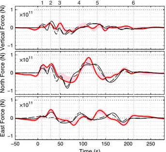
Figure 3. Force-time function from inversion of seismic data from all five
stations (thick red line) and using data from a single station, MRBL, the most distant station used (dashed-black line), demonstrating the stability of the solution, and 95% confidence interval of the solution estimated using multiple inversion with random decimation (pink area). The three collapses are labeled by numbers from 1 to 3. The first bend is between marks 3 and 4 and the second bend between marks 4 and 5. The number 6 marks the end of the force-time function.
the fact that data from just one three-component station gives very similar results to the solution obtained with five stations (Figure 3). This is true regardless of which station is used. However, in order to better assess how closely the forces predicted by our landslide simulations need to be to satisfactorily match the inversion result, we needed to formally assess the stability of the waveform inversion. To do this, we use a method similar to jackknife technique [Quenouille, 1956; Tukey, 1958] by reinverting the waveforms 200 times, but each time randomly excluding up to 9 of the 15 channels of data (from the five stations used) from the inversion (minimum of four and median of seven channels excluded). We employed the same methods as Allstadt [2013] to perform the waveform inversion except the filter used here is a second-order zero phase
Butterworth band-pass filter. We then took the middle 95% of the 200 inversion results at each time inter-val to generate an envelope representing a 95% certainty of where the solution lies. This was done for the period range T = 20 − 150 s (Figure 3). The uncertainty lies mainly in the amplitudes, while the phase and overall shape of the inversion is stable. Three peaks are clearly visible on the vertical component (labeled 1, 2, and 3 in Figure 3). On the east horizontal component, the third peak is less clear but nevertheless visible. It is slightly visible on the confidence interval of the North component, but not on the best inverted force-time function (red line).
2.3. Interpretation Based on a Simple Analysis
The first information provided by the force-time function is the duration of the primary movement of the landslide (about 200 s). It is almost certain that some material continued to move after that time, as indicated by the 5 min duration of the higher-frequency energy in the raw seismograms, but these final movements did not exert significant long-period forces on the ground surface (Figure 3).
The timing of the forces suggested that failure occurred progressively: the flank of the mountain first collapsed in two subhorizontal failures about 20 s apart, evidenced by two strong subhorizontal force pulses (labeled 1 and 2 in Figure 3). This was followed by a strong, nearly vertical force, suggesting that the evacuation of the flank material destabilized the steep Gendarme above, causing it to collapse almost vertically about 45 s after the start of the event (labeled 3 in Figure 3).
Considering the simple model of a rigid block sliding over a slope, Zhao et al. [2014] showed that it is possible to retrieve the mean slope angle of the source area using the formula
𝜃 = arctan (F z Fh ) (1) where Fzis the vertical force amplitude and Fhthe horizontal force amplitude. Assuming that the three peaks that appear at the beginning of the force-time function before the landslide turns into a debris flow are related to three different subevents and using equation (1), we obtain𝜃1= 13◦,𝜃2= 20◦, and 𝜃3= 62◦. This suggests that each successive failure occurred on a slope steeper than the previous one. The slope angle found for the third collapse supports the hypothesis of a third near-vertical collapse. Furthermore, using the formula on the entire 50 first seconds we obtain𝜃 = 23.4◦, while a mean slope angle of𝜃 = 23◦± 1◦is obtained from the postslide digital elevation model for the failure area resolved in the direction of failure [Allstadt, 2013].
An empirical estimate of the effective friction coefficient can be obtained from equation (S19) of Lucas et al. [2014] that predicts:𝜇 = V−0.0774, where V is the landslide volume. As a result, if we consider subevents, i.e., volumes of about 10–20 Mm3,𝜇 ∼ 0.29. To calculate the volume of each subevent, we use the formula derived from the sliding block model Brodsky et al. [2003]; Zhao et al. [2014] and the force amplitude Fhof the individual peaks that correspond to the three subevents (labeled 1, 2, and 3 in Figure 3):
V =|||| Fh
𝜌g cos 𝜃(𝜇 cos 𝜃 − sin 𝜃)||||, (2)
where V is the volume,𝜌 the density, g is acceleration due to gravity, and considering the confidence interval of the inverted force. We find volumes of 22.4 < V1 < 61.7 Mm3, 36 < V2 < 72.6 Mm3, and 2.8 < V3 < 5.8 Mm3, respectively, for the three collapses, for a total of 61 < V < 140 Mm3. Ekström and Stark [2013] also proposed an empirical relation between the force amplitude and the involved mass (V = 0.54 × F∕𝜌). Using their formula for the three collapse peaks, we obtain volumes of 6.7 < V1 < 18.3 Mm3, 12.5 < V2< 25.1 Mm3and 5.3 < V3< 10.8 Mm3, for a total of 24.5 < V < 54.2 Mm3. The volumes calculated following Zhao et al. [2014] are higher than those calculated following Ekström and Stark [2013], but both are of the same order of magnitude as the observations, which estimated a volume of 48.5 Mm3[Guthrie et al., 2012]. Using the mean value found for𝜃, we obtain a mean velocity U =√gh0cos𝜃 = 39 m/s [Lucas et al., 2014], which is consistent with the values found for the rockslide, before it turned into a debris flow [Allstadt, 2013, Figure 12].
To further interpret the forces obtained by waveform inversion and to improve our understanding of what can be resolved seismically and what cannot, we will simulate the landslide in the following sections and compare field observations (runout, runup) to numerical simulations results as well as the inverted to simulated force-time functions.
3. Numerical Modeling of the Mount Meager Landslide
3.1. The SHALTOP ModelWe simulated the Mount Meager landslide using the SHALTOP numerical model. This model describes homogeneous continuous granular flows over a 3-D topography z = b(x, y), where the horizontal/vertical coordinates are defined by (x, y, z) and x = (x, y) [Bouchut et al., 2003; Bouchut and Westdickenberg, 2004; Mangeney et al., 2007]. The model is based on a depth averaged thin layer approximation. It calculates the spatiotemporal flow thickness h(x, t) and the averaged velocity of the granular media utg(x, t) tangent to the topography. This tangent velocity is parameterized by its horizontal component u(x, t). The model takes into account the full curvature tensor of the topography
= cos3𝜃⎛⎜ ⎜ ⎝ 𝜕2b 𝜕x2 𝜕2b 𝜕x𝜕y 𝜕2b 𝜕x𝜕y 𝜕2b 𝜕y2 ⎞ ⎟ ⎟ ⎠ (3)
where𝜃(x, y) is the slope angle.
Using a Coulomb type friction law, the SHALTOP model has successfully reproduced experimental granular flows as well as natural landslides [Mangeney-Castelnau et al., 2005; Lucas and Mangeney, 2007; Kuo et al., 2009; Favreau et al., 2010; Lucas et al., 2011; Moretti et al., 2012; Lucas et al., 2014]. In this model the rheology involves only one parameter, the empirical friction coefficient𝜇 = tan 𝛿, where 𝛿 is the friction angle. The SHALTOP model describes the behavior of a granular material with mean frictional properties described by this empirical friction coefficient (see Lucas et al. [2014] for a detailed description of the friction coefficient). This coefficient is, for example, higher when the landslide flows over a rocky bedrock than over a glacier [Favreau et al., 2010]. Accurate simulation of debris flows would require the use of mixture (fluid grains) or two-phase flow models [e.g., Iverson and Denlinger, 2001; Pitman and Le, 2005; Pelanti et al., 2008, 2011; Bouchut et al., 2014]. However, as a first approximation, debris flows can be described by simply reducing the friction coefficient, we adopted this simple approach here as a first step to simulating the debris flow. Note that we decided here to use only one constant rheological parameter in this empirical approach even though the rheology of natural landslides and debris flows is obviously much more complicated. This choice was made because the flow law appropriate to describe natural landslides is still an open issue and the involved parameters are unknown. In particular, friction weakening is thought to occur in natural land-slides as suggested by seismic and field data [Lucas et al., 2014; Yamada et al., 2013]. Introducing friction weakening in landslide models seems to only weakly affect the generated seismic signal (M. Yamada et al., Estimation of dynamic friction process of the Akatani landslide based on the waveform inversion and numerical simulation, submitted to Geophysical Research Letters, 2014).
3.1.1. Force Calculation
The seismic waves associated with a landslide are generated by the variation of the force that it applies on the ground surface. The SHALTOP model calculates this force during the simulated flow that results from the complex balance between acceleration due to gravity, pressure gradients, frictional forces, inertia, and topography curvature effects. This calculated force has been shown to be capable of reproducing the long-period seismic waves associated with two large landslides [Favreau et al., 2010; Moretti et al., 2012]. Favreau et al. [2010] and Moretti et al. [2012] showed that this force is very sensitive to landslide dynamics (flow history) and can be used to discriminate between different scenarios. In order to strictly preserve the force balance between the initial and final states, third-order terms in the thin layer asymptotic develop-ment have been taken into account [Moretti et al., 2012]. However, contrary to Moretti et al. [2012] the force is calculated based on the conservative term hu to appropriately account for velocity discontinuities in hyperbolic equations. The time-dependent three-component stress field associated with this force is calculated as follows: ⃗T(x, t) = −Pbottom⃗n + c𝜌𝜇 ((𝜕hI)u)tg √ c2|u|2+ (s⋅ u)2 ( 1 +u tu gc ) + , (4)
where Pbottomis the pressure at the bottom of the landslide and is expressed as Pbottom=𝜌gch + 𝜌hutu − 𝜌𝜕t
( h2 2∇x⋅ (cu) ) −𝜌∇x⋅ ( h2 2cu∇x⋅ (cu) ) . (5)
Table 1. Tested Values of Simulation Parametersa
Parameters Tested Values
t2 10, 20 , and 30 s
t3 20, 30 , and 40 s
𝜇 = tan 𝛿 [0.23, 0.44] = tan([13, 24]◦);𝛿 ∈ N
𝜇df= tan𝛿df [0.10, 0.21] = tan([6, 12]◦);𝛿df∈N
Released areas see Figure 4
at
2is the time when the second collapse occurs,t3is the time when
the third collapse occurs,𝜇is the friction coefficient of the rockslide, and
𝜇dfis the friction coefficient of the debris flow.
⃗n(x) = (−s, c) is the upward unit vector normal to the topography,
s=√ ∇xb
1+||∇xb||2
,= cos𝜃, Vtg=(V, stV∕c) with V any two-dimensional horizontal vector, (a)+= max(0, a), g is the acceleration due to gravity,𝜌 is the flow density, and
𝜕hI(x, h) = ∫ h 0 det(Id −𝜉𝜕xs) (Id −𝜉𝜕xs)−1gcd𝜉 (6)
where det is the determinant of a given matrix and Id is the identity matrix. The force applied by the landslide to the ground surface as a function of time ⃗F(t) is obtained by integrating the stress field ⃗T(x, t) over the surface area with dS = dx∕c the surface unit:
⃗F(t) = ∫S ⃗T dS = ∫x ⃗T(x, t)dx c . (7) 3.2. Landslide Simulations
3.2.1. Comparison With Field Observations Alone
In this section, we test different scenarios to support or invalidate former interpretations of the landslide dynamics discussed in section 2.3 and to provide quantitative estimates of the initial conditions (volume and timing of the released mass) and of the friction coefficients characterizing dissipation during the flow. The parameters tested are the number, timing, and volume of subevents and the friction coefficient of both the rockslide and the debris flow. All the tested scenarios are summarized in Table 1 and Figure 4, the volume ratio of each collapses on each scenario is given in Table S1 in supporting information.
5000 6000 7000 2000 5000 6000 7000 2000 5000 6000 7000 2000 5000 6000 7000 2000 5000 6000 7000 2000 5000 6000 7000 2000 5000 6000 7000 2000 5000 6000 7000 2000 5000 6000 7000 2000 5000 6000 7000 2000
1 c
ollapse
2 c
ollapses
3 c
ollapses
(a)
(f )
(e)
(d)
(c)
(b)
(j)
(i)
(h)
(g)
Figure 4. Simulated scenarios for (a) 1, (b–f ) 2, and (g–j) 3 collapses. The colors represent the area corresponding to the different failures. Light blue represents
the mass that collapses at timet = 0s, yellow represents the mass that collapses at timet = t2, and red represents the mass that collapses at timet = t3. Purple
2000 3000 4000 5000 6000 2000 4000 6000 8000 10000 2000 3000 4000 5000 6000 2000 4000 6000 8000 10000 2000 3000 4000 5000 6000 2000 4000 6000 8000 10000 2000 3000 4000 5000 6000 2000 4000 6000 8000 10000 2000 3000 4000 5000 6000 2000 4000 6000 8000 10000 2000 3000 4000 5000 6000 2000 4000 6000 8000 10000 2000 3000 4000 5000 6000 2000 4000 6000 8000 10000 2000 3000 4000 5000 6000 2000 4000 6000 8000 10000 2000 3000 4000 5000 6000 2000 4000 6000 8000 10000 2000 3000 4000 5000 6000 2000 4000 6000 8000 10000 2000 3000 4000 5000 6000 2000 4000 6000 8000 10000 2000 3000 4000 5000 6000 2000 4000 6000 8000 10000
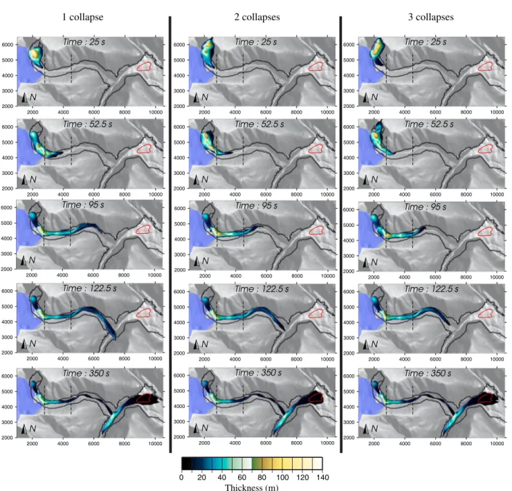
1 collapse
2 collapses
3 collapses
0 20 40 60 80 100 120 140 Thickness (m) 2000 3000 4000 5000 6000 2000 4000 6000 8000 10000 2000 3000 4000 5000 6000 2000 4000 6000 8000 10000 2000 3000 4000 5000 6000 2000 4000 6000 8000 10000
Comparison with field observations
Figure 5. Snapshots of the simulations that best fit depositional observations for, the scenarios with (left) one collapse att1 = 0s, (middle) two collapses at
t1= 0s andt2= 20s, and (right) three collapses att1= 0s,t2= 20s, andt3= 40s (right). For all the simulations, the friction coefficients are𝜇 = tan(18◦) = 0.32,
𝜇df = tan(8◦) = 0.14, and𝜇g= tan(5◦) = 0.11. Capricorn glacier is shown in violet. The two vertical black dashed lines represent the distance over which the
landslide transforms into a debris flow: the friction coefficient linearly decreases from𝜇at the first left dashed line to𝜇dfat the second right dashed line. The red
outline corresponds to the approximate location of the plug where the dry front stopped [see Guthrie et al., 2012, Figure 14].
We describe the debris flow by spatially reducing the basal friction coefficient linearly from𝜇 to 𝜇dfover a distance of about 1.5 km along Capricorn Creek downstream from the source area (see vertical dashed lines in Figure 5). This ad hoc assumption is the simplest way to reduce progressively the friction coefficient where the rockslide changes into a debris flows. The Capricorn Glacier is also taken into account by simply reducing the friction coefficient to𝜇g = tan(5◦) = 0.11 when the avalanche passes over it [Favreau et al., 2010; Moretti et al., 2012]. Due to the short distance traveled over the glacier, a small variation of𝜇ghas a very weak influence on the dynamics.
One Single Collapse. Considering one single collapse (Figure 4a) and taking into account the debris flow, we are able to reproduce the traveled distance with a friction coefficient for the rockslide of𝜇 = 0.32 (Figure 5, left) and a friction coefficient for the debris flows𝜇df = tan 8◦ = 0.14. Note that when the debris flow is not considered, i.e., keeping the same friction coefficient for the rockslide and the debris flow, a friction coefficient of𝜇 = tan(13.5◦) = 0.24 is necessary just to make the landslide reach the Meager Creek valley wall.
Two Collapses. We then performed simulations considering two collapses. We set the first to occur at the beginning of the simulation and the second at time t2. Figure 5 (middle) shows the simulation for t2= 20 s. As Allstadt [2013] suggested that the events should be separated by about 20 s, we performed different simulations using t2 = 10, 20, and 30 s. We also tried different volume ratios between the first and the second collapsing parts of the mass (Figures 4b–4f ). Whatever the scenario, the landslide deposit is very similar to that of the scenario with a single collapse (Figure 5, left, and 5, middle). However, the dynamics are different. In particular, the flow front runs faster with a single collapse and the peaks (maximum elevation) of the mass are not always located at the same position (e.g., see time t = 52.5 s in Figures 5 (left) and 5 (middle)).
Three Collapses. To test the hypothesis of a third collapse, we repeated the previous simulations but consid-ering three subevents instead of two. Here a part of the mass is released at the beginning of the simulation, another part at time t = t2, and a third part at time t = t3. Figure 5 (right) shows the simulation for t2= 20 s and t3= 40 s. We performed different simulations with t2= 10, 20, and 30 s and t3= 20, 30, and 40s for the scenarios given in Figures 4g–4j). As before, these different scenarios give very similar runout distances and deposit areas. As a result, it is not possible to discriminate the scenarios using just depositional measure-ments. By choosing a rockslide friction coefficient𝜇 between 0.24 and 0.45, the runup on the Meager Creek valley wall constrains𝜇dfto a value between 0.13 and 0.16. In all the tested scenarios, the runout and the runup can be fit by adjusting the friction coefficients.
Whatever the scenario, we fit the primary deposit runout distance related to the first drier front that stopped about 10 km from the source area (see plug in Figure 5). Contrary to Guthrie et al. [2012], we do not repro-duce the total runout distance that is expected to be due to further remobilization of the first deposit by wetter flows as discussed in section 2.1 and by Guthrie et al. [2012]. This may be partially because we do not model water entrainment when the debris flow travels into Meager Creek. This may explain the differences between their estimated friction coefficient and ours.
Our results show that the constraints imposed by the runup and runout distances measured in the field and in satellite imagery do not allow us to determine the number and timing of the subevents in the different scenarios. Indeed, these observations can be easily fit by varying the friction angles of the rockslide or debris flow.
3.2.2. Comparison Between Calculated and Inverted Force History
Contrary to field observations, the inverted force-time function contains timing information. In this section, we present the comparison between the forces inverted from the long-period seismograms (Figure 3) and the forces calculated for the scenarios presented above in the period range T ∈ [20, 150] s. In order to determine the scenario that best fits the observed landslide flow history, we calculated, for each component of the force, the correlation between the simulated and the inverted force:
C = N ∑ i=1 (di− ̄d)⋅ (si−̄s) √ N ∑ i=1 (di− ̄d)2⋅ √ N ∑ i=1 (si−̄s)2 (8)
where d and s are the two signals for which the correlation is calculated. Then we calculated a weighted mean of the correlations, each component of the force being weighted by its maximum amplitude. We did the same with the misfit
misfit = 1 |dmax− dmin| √ √ √ √ 1 N N ∑ i=1 (di− si)2 (9)
Table 2. Correlation and Misfit Values for the Scenarios That Best Fit the
Inverted Force-Time Function for 1, 2, and 3 Collapsesa
Correlation Normalized Misfit Vertical North East Vertical North East One collapse 0.06 -0.16 0.18 0.32 0.26 0.28 Two collapse 0.12 0.66 0.1 0.33 0.15 0.22 Three collapse 0.44 0.75 0.45 0.19 0.11 0.15
aThey correspond to the scenarios represented in Figures 6, 7, and 9.
The correlation represents how the phase is reproduced while the misfit takes into account the amplitude of the signals. The best scenario is defined as that which has the maxi-mum weighted mean correlation and the minimum weighted mean misfit. The simulations corresponding to the best scenarios for one, two, and three collapses are shown in Figure 7. For these scenarios, the values of the misfit and correlation for each component of the force are shown in Table 2. Figure 6 compares the forces simulated with the best one-, two-, and three-collapse scenarios with the inverted force.
One Single Collapse. Figure 6 shows that assuming a single collapsegenerates, on every component, only one force peak with high amplitude during the first 50 s (black dotted lines), which is not consistent with the inverted force that exhibits two to three peaks (red lines). The force history at later times t = 50 − 100 s is also very different from the inverted forces on every components. After t = 100 s, the force is approx-imately in the range of the inverted forces. Note that it is very important to look at all the components of the force to compare the simulated and observed forces. For example, looking only at the vertical component would suggest that the flow dynamics from t = 40 − 60 s is roughly reproduced, while the east and north components show the opposite. Assuming one single collapse, the best fit of the forces is obtained with𝜇 = tan 21◦ = 0.38 and 𝜇df = tan 11◦ = 0.19. However, Figure 7 shows that with this scenario the deposits are poorly reproduced compared to those produced by the scenarios with two or three collapses. Indeed, the correlation is lower than 0.18 and the misfit larger than 0.28 (see Table 2).
−50 0 50 100 150 200 250 −1 0 1 Time (s) East Force (N) ×1011 −1 0 1 North Force (N) ×1011 −1 0 1 1011 Vertical Force (N) × 1 2 3 4 5 6 1 collapse 2 collapses 3 collapses
Figure 6. Force applied by the landslide to the ground surface. The
different lines represent the inverted force (red), the force corresponding to the best scenarios represented in Figure 5: for one (black dotted line), two (black dashed line), and three (black solid line) collapses. The light pink area represents the 95% confidence interval of the inversion. The force-time functions are filtered between 20 and 150 s. The vertical dashed-gray lines are located at the position of the different peaks of the force that are numbered on top of the Figure. As in Figure 3, the first bend is marked between labels 3 and 4 and the second bend between labels 4 and 5. The number 6 marks the end of the force-time function.
Two collapses. Let us now consider two collapses (black dashed lines in Figure 6). The best fit of the inverted force is obtained for the scenario for which𝜇 = tan 18◦ = 0.33, 𝜇df = tan 8◦= 0.14, and t2= 20 s and for which the area corresponding to the two collapses are shown in Figure 4d. This scenario clearly reproduces the two peaks on the north and east components. However, the third peak on the vertical com-ponent does not appear. With two collapses, the amplitude of the second peak on the vertical and north components is overestimated. From t = 30 − 100 s, the simulated force has an amplitude and phase different from the inverted force. At later times, the simulated force is roughly in the range of the inverted force. Regarding the velocities and the deposits (Figure 7), this scenario is very differ-ent, in terms of runout, depositional area, and velocity, than the one that best fits the force considering one single collapse and fits the deposits better. The correlation of the best two-collapse scenario is better than
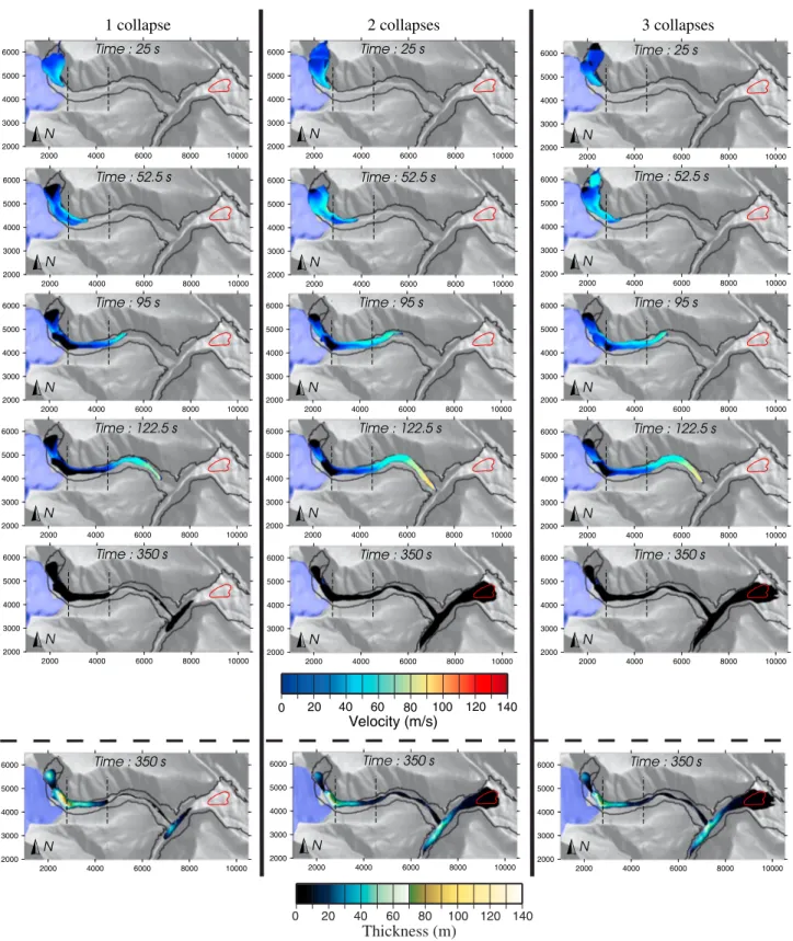
1 collapse
2 collapses
3 collapses
2000 3000 4000 5000 6000 2000 4000 6000 8000 10000 2000 3000 4000 5000 6000 2000 4000 6000 8000 10000 2000 3000 4000 5000 6000 2000 4000 6000 8000 10000 2000 3000 4000 5000 6000 2000 4000 6000 8000 10000 2000 3000 4000 5000 6000 2000 4000 6000 8000 10000 2000 3000 4000 5000 6000 2000 4000 6000 8000 10000 2000 3000 4000 5000 6000 2000 4000 6000 8000 10000 2000 3000 4000 5000 6000 2000 4000 6000 8000 10000 2000 3000 4000 5000 6000 2000 4000 6000 8000 10000 2000 3000 4000 5000 6000 2000 4000 6000 8000 10000 2000 3000 4000 5000 6000 2000 4000 6000 8000 10000 2000 3000 4000 5000 6000 2000 4000 6000 8000 10000 2000 3000 4000 5000 6000 2000 4000 6000 8000 10000 2000 3000 4000 5000 6000 2000 4000 6000 8000 10000 2000 3000 4000 5000 6000 2000 4000 6000 8000 10000 2000 3000 4000 5000 6000 2000 4000 6000 8000 10000 2000 3000 4000 5000 6000 2000 4000 6000 8000 10000 2000 3000 4000 5000 6000 2000 4000 6000 8000 10000 0 20 40 60 80 100 120 140Thickness (m)
0 20 40 60 80 100 120 140 Velocity (m/s)Comparison with the inverted force history
Figure 7. Velocities and deposits corresponding to the simulations that best fit the inverted force-time function for 1, 2, and 3 collapses. The scenario with
(left column) one collapse corresponds to𝜇 = 0.38and𝜇df = 0.19. The scenario with (middle column) two collapses corresponds to𝜇 = 0.33,𝜇df = 0.14and
t2 = 20s. The scenario with (right column) three collapses corresponds to𝜇 = 0.33,𝜇df = 0.14,t2= 20s, andt3= 40s. The two vertical black dashed lines represent the distance over which the landslide turns into a debris flow: the friction coefficient linearly decreases from𝜇at the first (left) line to𝜇dfat the second (right) line. The red outline corresponds to the approximate location of the plug where the dry front stopped [see Guthrie et al., 2012, Figure 14].
−50 0 50 100 150 200 250 −1 0 1 East Force (N) Time (s) ×1011 × −1 0 1 North Force (N) ×1011 × −1 0 1 ×10¹¹ Vertical Force (N) × 1 2 3 4 5 6
Figure 8. Force applied by the landslide to the ground surface. The
dif-ferent lines represent the inverted force (red), the force corresponding to the best scenario (black solid line) and to the same scenario but with the collapsing areas represented by Figure 4i instead of Figure 4j (black dashed lines). The light pink area represents the 95% confidence inter-val of the inversion. The force-time functions are filtered between 20 and 150 s. The vertical dashed-gray lines are located at the position of the different peaks of the force that are numbered on top of the Figure.
for one-collapse except on the east component of the force and the misfit is smaller except for the vertical component (Table 2).
Three Collapses. By considering three collapses (black solid lines in Figure 6), we obtain a reasonable agreement with the data for the three force components. This scenario is quite similar to the one with two collapses (Figure 7). Indeed, for these two scenarios, the velocities are very similar and for each point in time, the frontal velocity is about 20 m/s higher than that of the center of mass, with a maximum value of about 90 m/s. However, the force-time function corresponding to three collapses fits the inversion better, especially on the ver-tical component (Figure 6). Indeed, the three first peaks (labeled 1, 2, and 3 in Figure 6) on the vertical component are reproduced, while a third peak at t ≃ 50 s is also obtained in the simulated force on the north component, although this peak is not visible on the best inverted force (red line). However, a third peak on the north component is distinguishable on the maximum value of the confidence interval of the inverted force. This shows how important it is to calculate such confidence intervals. Between t = 60 s and t = 80 s, the simulated force is quite different from the inverted force: a small peak is simulated but not observed at 70 s on the vertical force, a stronger and more localized minimum is simulated around 65 s on the north force and the observed minimum at 80 s on the east force is not simulated. This time interval corresponds to the ad hoc empirical transition between the friction coefficient𝜇 and 𝜇df(see dashed-black lines on Figure 7). After about t ≈ 110 s, the scenarios with two or three initial collapses become very similar. After 110 s, even if the simulated force is close to the inverted force, the small peaks are not accurately reproduced and there are phase shifts, especially on the east component after t ≈ 120 − 130 s. This corresponds to the arrival of the flow in Meager Creek. However, this part of the flow cannot be accurately simulated using our single-phase flow model. The best three-collapse scenario has significantly higher correlation (>0.44) and smaller misfit (<0.19) than the other scenarios for all the components of the force (Table 2).
For the scenarios with two or three collapses, simulations show that most of the deposits are emplaced after t ≈ 280 s. However, a small part of the landslide, with a small thickness, is still in movement until t ≈ 350 s. Figure 6 shows that these few remaining movements do not produce a significant force after t≳220 s which is consistent with seismic data. Note that using four collapses generate four peaks in the simulated force which is not consistent with the inverted force.
3.3. Best Simulated Scenario 3.3.1. Flow Dynamics
Here we look for the model that best fits both the forces (i.e., minimizes misfit and maximizes correlation) and the field observations, i.e., the landslide flow history, the runup distance, and the runout distance. This scenario is the same as that which best fits the force-time function and consists of three collapses that occur successively at times: t1 = 0 s, t2 = 20 s and t3 = 40 s, with volumes V1 = 14 Mm3, V
2 = 27.5 Mm3, and V3 = 7 Mm3, respectively. These volume values are very consistent with those found using the empirical laws of Ekström and Stark [2013] and that of Zhao et al. [2014] (see section 2.3). The best fitting values of the friction coefficient of the rockslide is𝜇 = tan(18◦) = 0.33 and that of the debris flow is 𝜇df= tan(8◦) = 0.14. When considering scenario represented in Figure 4i, the second peak visible on the east component of the
2000 3000 4000 5000 6000 7000 2000 4000 6000 8000 10000 2000 3000 4000 5000 6000 7000 2000 4000 6000 8000 10000 2000 3000 4000 5000 6000 7000 2000 4000 6000 8000 10000 2000 3000 4000 5000 6000 7000 2000 4000 6000 8000 10000 2000 3000 4000 5000 6000 7000 2000 4000 6000 8000 10000 2000 3000 4000 5000 6000 7000 2000 4000 6000 8000 10000 2000 3000 4000 5000 6000 7000 2000 4000 6000 8000 10000 2000 3000 4000 5000 6000 7000 2000 4000 6000 8000 10000 0 20 40 60 80 100 120 140 Thickness (m) Force : 3.2×10 10 N Velocity : 50 m/s
Scale :
(a)
(b)
(d)
(c)
(f )
(h)
(e)
(g)
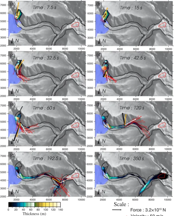
Figure 9. Snapshots of the best scenario simulation. The red arrows represent the velocity field, the black dot is the
center of mass, the white arrow is the mean velocity of the center of mass and the black (simulated) and orange (inverted) arrows represent the horizontal force applied to the ground. Capricorn glacier is represented in violet. The scale of the white arrows is the same as the red arrows and the orange arrows are scaled the same as the black arrows. The red outline corresponds to the approximate location of the plug where the dry front stopped (see [Guthrie et al., 2012] their Figure 14). The mean velocity is calculated by averaging the velocities within 100 m of the center of mass.
force at t ≈ 30 s (labeled 2 in Figure 8) is not well reproduced by the simulation (see dashed line on Figure 8). This peak, corresponding to the second collapse accelerating in the west direction, can only be reproduced with the scenario shown in Figure 4j. In that case, the left part of the mass (blue in Figure 4) collapse first, leaving this area empty and so allowing the rest of the mass to collapse in the west direction (Figure 9c). Scenario represented in Figure 4j reproduces the second peak on the east component well.
The simulated runup ru = 266 m on the Meager Creek valley wall is very close to the observed runup ru= 270 m (black line in Figure 10). Furthermore, this scenario well reproduces the height of the deposits
0 50 100 150 200 250 300 350 0
200 400
Observed runup (ru=270 m)
Figure 10. Runup calculated by the SHALTOP model on the Meager
Creek valley wall for the best scenario (black solid line) and for different debris flow friction coefficients:𝛿df=6.4◦(green), 7.2◦(dashed green), 8◦(black), 8.8◦(dashed blue), and 9.6◦(blue). The black line represents the runup corresponding to the best calculated scenario. The black dashed line represents the value of the observed runup.
near the source area (Figures 1 and 9). Indeed, field observations show a maximum depositional height of 29 m and the simulation predicts a maximum height of 31 m in this area.
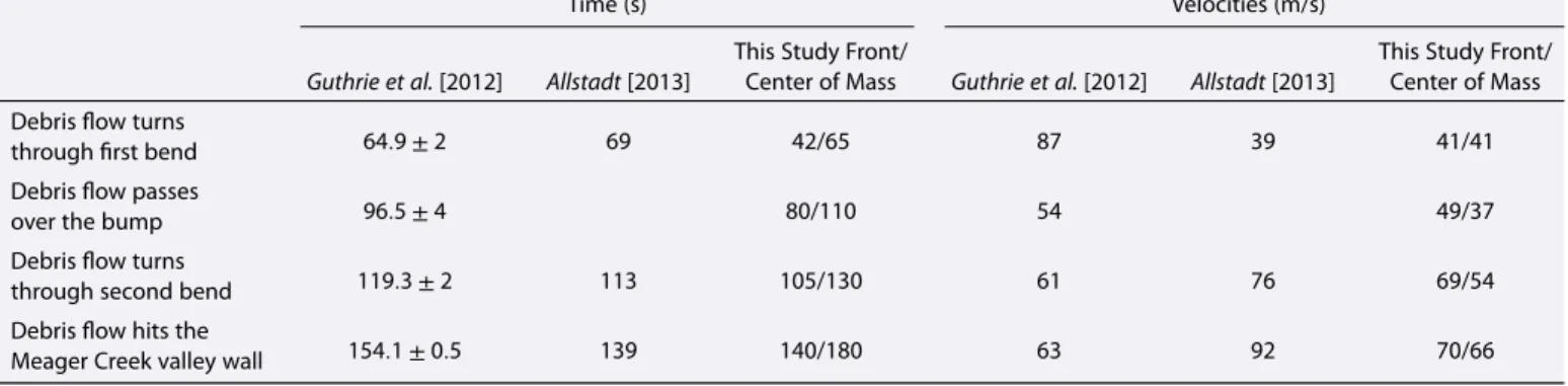
The velocities and timing correspond-ing to this scenario compare favorably with the values obtained by Guthrie et al. [2012] and Allstadt [2013] using simpler analyses (Figure 11 and Table 3). We see that at the very beginning (before 1 km) and at the end (after 8 km), the simulated frontal velocity (blue line on Figure 11) is closer to that obtained by Guthrie et al. [2012] using analysis of raw seismograms (black line) than to that obtained by Allstadt [2013] using seis-mic inversion (red line), while this is the contrary for the mean velocity. During the middle of the flow, the frontal velocity is roughly closer to that obtained using seismic inversion. However, the simulations provide much more detailed information on the velocity fluctuation during the flow. The frontal velocity increases suddenly during the first 500–1000 m up to 45 m/s, which corresponds to its acceleration as it passes over the glacier. Then, when the mass returns to the bedrock substrate, the velocity decreases over a distance of about 1000 m. At a distance of about 2000 m along the path, where the landslide turns into a debris flow, the velocity of the mass increases, then drastically decreases at a distance of about 6500 m when the mass begins its runup on the Meager valley wall. Except for the first 2000 m, the velocity of the center of mass exhibits a very similar shape to that of the front. The difference observed along the first 2000 m may be due to the fact that a large amount of mass stops just after passing the glacier as shown in the simulations. 3.3.2. Interpretation of the Force History
Figure 9 shows, during the different stages of the simulation, the force, the velocity field, and the mean velocity of the center of mass. The first stage of the force is associated with an initial acceleration of the mass toward the southwest (i.e., in the opposite direction of the force) as shown in Figures 9a–9c. After the collapses, on the north component, we observe a negative force (i.e., toward the south) on both the inverted and simulated force-time function between times 40 and 95 s (see Figures 9d and 9e). This corresponds to
0 2000 4000 6000 8000 10000 0 20 40 60 80 100 120
Figure 11. Velocity of the landslide versus horizontal distance
trav-eled. The black line is from Guthrie et al. [2012] and represents the frontal velocity. The red line results from the interpretation of the inversion of the seismic signal [Allstadt, 2013] and is representative of the center of mass velocity. Frontal (blue) and center of mass (green) mean velocities calculated by the SHALTOP model for the best landslide scenario. The timing and mean values of the veloci-ties up to each landmark along the path are reported in Table 3. The mean velocity is calculated by averaging the velocities within 100 m of the center of mass/front.
the time when the center of mass is located within the first bend of the valley (Figure 9). Then, between times 95 and 130 s, the inverted force is positive (i.e., toward the north) as illustrated in Figures 9e– 9f. The simulation shows that at that time (between times 100 and 150 s), the center of mass is located within the second bend that has a curvature in the opposite direction of the first bend. At time 130 s, the front arrives in the Meager Creek and runs up the opposite flank. This may correspond to the last peak on the vertical component of the inverted force but this is not clearly visible on the simulated force.
The east component of the force is also well reproduced (Figures 6 and 9). First, the three collapses occur before time t = 50 s, and the force is mainly eastward, in the opposite direction of the initial acceleration of the mass. Then the flow is mostly directed toward the east. Between 50 and 90 s, the force is mainly westward and can be
Table 3. Timing and Mean Velocities of the Front and the Center of Mass of the Landslide Compared to Values Given in Guthrie et al. [2012] (Frontal) and
Allstadt [2013] (Center of Mass)
Time (s) Velocities (m/s)
This Study Front/ This Study Front/ Guthrie et al. [2012] Allstadt [2013] Center of Mass Guthrie et al. [2012] Allstadt [2013] Center of Mass Debris flow turns
64.9 ± 2 69 42/65 87 39 41/41
through first bend Debris flow passes
96.5 ± 4 80/110 54 49/37
over the bump Debris flow turns
119.3 ± 2 113 105/130 61 76 69/54
through second bend Debris flow hits the
154.1 ± 0.5 139 140/180 63 92 70/66
Meager Creek valley wall
associated with a phase of acceleration of a mass. Later on, between 120 and 160 s, the main part of the mass decelerates and the resulting force is directed toward the east. Note that the mean velocity of the flow is not in the same direction as the force (Figures 9f and 9g).
3.4. Sensitivity Study of the Simulated Force
In the following, we present the sensitivity of the force to the different parameters involved (volume and friction coefficients). For each parameter, we tried different values, while fixing the other parameters to the value corresponding to the best scenario described above.
3.4.1. Volume
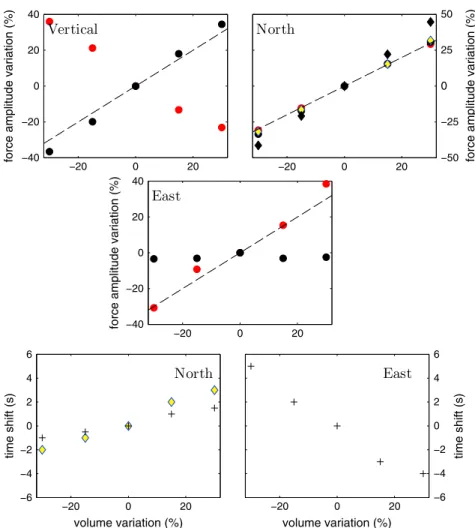
We varied the volume by keeping the same reconstructed mass shape, changing only its height, the same volume proportions are kept between the subevents. As there is at least 15% uncertainty in the total land-slide mass estimates, we varied the volume by ±15% and by ±30%. The volumes tested are thus 34 Mm3, 41.2 Mm3, 48.5 Mm3, 55.7 Mm3, and 63 Mm3. Figure 12 shows the force-time function corresponding to these different scenarios and Figure 13 shows how the amplitude and the timing of the peaks observable on these force-time functions vary. Figures 12 and 13 show a linear relation between force amplitude and
−50 0 50 100 150 200 250 −1 0 1 East Force (N) Time (s) ×1011 ×1011 ×1011 ×1011 ×1011 −1 0 1 North Force (N) ×1011 ×1011 ×1011 ×1011 ×1011 −1 0 1 ×10¹¹ Vertical Force (N) ×1011 ×1011 ×1011 ×1011 + 34 Mm 41.2 Mm 55.7 Mm 63 Mm 48.5 Mm waveform inversion
Figure 12. Sensitivity of the force-time function to the volume
involved. The lines correspond toV = 34Mm3(green), 41.2 Mm3
(dashed green), 48.5 Mm3(black), 55.7 Mm3(dashed blue), and
63 Mm3(blue). The red line corresponds to the best inverted force
and the pink area is the confidence interval. The markers represents the peaks of the force analyzed in Figure 13.
volume, as an example, an increase of 30% of the volume implies a variation of 31% ± 5% in the amplitude of the force peaks that correspond to the first and second subevents, as predicted by the law proposed by Ekström and Stark [2013]. The force peak that corresponds to the third subevent shows a more complicated behavior, probably because the signature of the third collapsing mass is mixed up with that of the mass that is already flowing downslope. However, the first peak of the vertical com-ponent of the force (red dots in Figures 12 and 13), shows a behavior opposed to the other peaks, i.e., an increase in the volume corresponds to a decrease in the force amplitude. The second peak (black dots) of the east component presents a very slight variation. These behaviors show the strong impact of the topography on the force applied to the ground surface. The most important changes appear on the north component of the force at time t ∼ 110 s: at this time, a change of 30% in the volume implies a variation of 50% in the maximum
−20 0 20 −40 −20 0 20 40
force amplitude variation (%)
−20 0 20 −50
−25 0 25 50
force amplitude variation (%)
−20 0 20 −40 −20 0 20 40
force amplitude variation (%)
−20 0 20 −6 −4 −2 0 2 4 6 volume variation (%) time shift (s) −20 0 20 −6 −4 −2 0 2 4 6 volume variation (%) time shift (s)
Figure 13. Variations of the force amplitude and phase shifts corresponding to variations of±15% and±30% of the volume. The dashed line represents the linear variation predicted by the law proposed by Ekström and Stark [2013]
(M = 0.54 × F). The markers correspond to the peaks shown in Figure 12.
amplitude (black diamonds in Figures 12 and 13). This corresponds to the time when the landslide turns through the second bend. This shows that the maximum of the force here is not proportional to the involved volume as proposed by Ekström and Stark [2013]. By chance, this maximum force in the north direction here corresponds to the sum of the first two peaks and therefore leads to the right volume. A phase shift is also observed (Figure 13) when the volume is changed. For example, on the north and east components of the force, a shift of 5 s is observed for a variation of 15% in the volume (t ≈ 160 s).
3.4.2. Rockslide Friction Coefficient
We now vary the friction coefficient of the rockslide, i.e., at the beginning of the simulation. We chose to vary the estimated value (𝜇 = 0.33) of the friction coefficient by ±10% and ±20%. The tested values are therefore 𝜇 = 0.26 (𝛿 = 14.6◦),𝜇 = 0.29 (𝛿 = 16.3◦),𝜇 = 0.33 (𝛿 = 18◦),𝜇 = 0.36 (𝛿 = 19.7◦), and𝜇 = 0.39 (𝛿 = 21.3◦). As for the volume variations, Figures 14 and 15 show the force-time functions corresponding to these different simulations and how the amplitude and timing of the peaks varies. These figures show that the force is more sensitive to the rockslide friction coefficient than to the volume. For example, a decrease of 20% in the friction coefficient results in an increase of 35% ± 12% in the amplitude of the force peaks that correspond to the first and second subevents. The force peak that corresponds to the third subevent shows a more complicated behavior, probably because the signature of the third collapsing mass is mixed up with that of the mass that is already flowing downslope. These variations of amplitude are consistent with equation (2) for the range of values of𝜃 and 𝜇 considered here. As for the variation of volume, the first peak of the vertical component of the force (red dots in Figures 14 and 15) exhibits a behavior opposite to the other peaks. Similar to the volume sensitivity, the amplitude variations are greater at times t ≃ 65 and 110 s, when the flow turns through the bend. We also observe that for the highest friction coefficients, the
−50 0 50 100 150 200 250 −1 0 1 East Force (N) Time (s) ×1011 ×1011 ×1011 ×1011 ×1011 −1 0 1 North Force (N) ×1011 ×1011 ×1011 ×1011 ×1011 −1 0 1 ×10¹¹ Vertical Force (N) ×1011 ×1011 ×1011 ×1011 =14.6° =16.3° =19.7° =21.3° =18° waveform inversion +
Figure 14. Sensitivity of the force-time function to the rockslide friction coefficient. The lines correspond to𝛿 = 14.6◦, (green) 16.3◦(dashed green), 18◦(black), 19.7◦(dashed blue), and 21.3◦(blue). The red line corresponds to the best inverted force and the pink area is the confidence interval. The markers represents the peaks of the force analyzed in Figure 15. 0.250 0.3 0.35 0.4 0.2 0.4 force amplitude ( × 10 11 N) force amplitude ( × 10 11 N) force amplitude ( × 10 11 N) 0.25 0.3 0.35 0.4−1.5 −1 −0.5 0 0.5 1 0.25 0.3 0.35 0.4 −0.2 0 0.2 0.4 0.6 friction coefficient 0.25 0.3 0.35 0.4 −30 −20 −10 0 10 20 30 friction coefficient time shift (s) 0.25 0.3 0.35 0.4−30 −20 −10 0 10 20 30 friction coefficient time shift (s)
Figure 15. Variations of the force amplitude and phase shifts corresponding to variations of±10% and±20% of the rockslide friction coefficient𝜇. The markers correspond to the peaks shown in Figure 14.
−50 0 50 100 150 200 250 −1 0 1 East Force (N) Time (s) ×1011 ×1011 ×1011 ×1011 ×1011 −1 0 1 North Force (N) ×1011 ×1011 ×1011 ×1011 ×1011 −1 0 1 ×10¹¹ Vertical Force (N) ×1011 ×1011 ×1011 ×1011 δdf=6.4° δdf=7.2° δdf=8.8° δdf=9.6° δdf=8° waveform inversion
Figure 16. Sensitivity of the force-time function to the debris flow friction coefficient. The lines correspond to𝛿df= 6.4◦
(green), 7.2◦(dashed green), 8◦(black) , 8.8◦(dashed blue), and 9.6◦(blue). The red line corresponds to the best inverted force and the pink area is the confidence interval.
force amplitude reduces drastically after the second turn, meaning that the main part of the landslide stops too soon because most of the mass remains blocked at the top of the slope, just after Capricorn Glacier. As for the volume, phase shifts are observed between the different values of the friction coefficient (Figure 15). For example, on the north component, a shift of 10 s is observed for a variation of 15% in the friction coefficient (t ≈ 160 s). These phase shifts are due to the fact that reducing the friction coefficient increases the velocity of the landslide, causing it to arrive earlier at the different stages of the topography (e.g., bends). This implies that phase shifts are greater at the end of the force than at the beginning (Figure 15).
3.4.3. Debris Fow Friction Coefficient
We tested the sensitivity of the debris flow friction coefficient by changing its value by ±10% and ±20%, i.e., 𝜇df = 0.11 (𝛿df= 6.4◦),𝜇df= 0.13 (𝛿df = 7.2◦),𝜇df= 0.14 (𝛿df = 8◦),𝜇df = 0.15 (𝛿df= 8.8◦), and𝜇df= 0.17 (𝛿df = 9.6◦). Contrary to the rockslide friction coefficient, the debris flow friction coefficient has only a weak influence on the simulated force (Figure 16). On the other hand, the runup is very sensitive to this parameter. Changing the friction angle by 20%, changes the runup distance by about 35% (simulated runup ru=175 m) (Figure 10).
4. Link With the Broadband Seismic Signal
In this section, we compare the spectrogram of the vertical component of the seismic signal recorded at the closest broadband seismic station located 70 km from the Mount Meager (WSLR in Figures 1 and 2) to the long-period inverted force and to the landslide dynamics corresponding to the simulations that best fit the observations (Figure 17). As assumed by Guthrie et al. [2012], the different peaks of seismic energy of the spectrogram, visible on Figure 17, correspond to the slide material hitting and passing bumps and passing through bends. Few energy, long-period (T≥ 8 s) peaks appear on the spectrogram before t < 40 s. These small peaks correspond perfectly to the peaks of the long-period inverted force that represent the first and second collapses. Then another low-frequency peak (T > 5 s) appears at time t = 42 s, which corresponds also perfectly to the third peak on the force and to the third collapse. This time is the beginning of the high frequencies, probably because this is when rocks begin to break up into a flow and smaller-scale momentum exchanges start to become significant. This breaking could be very strong because the third collapse is almost vertical. A peak at t = 80 s appears only at high frequencies (T< 4 s) and seems to cor-respond to the front of the landslide passing over a bump (see Figure 1), i.e., to small-scale topography. Another peak in the spectrogram begins at time t = 117 s, corresponding to a peak in the horizontal components of the force and related to the second bend. Then another broader band peak occurs at time t = 145 s associated with a significant variation of the vertical and north components of the force. It seems
0 Vertical 0 North 0 East Time (s) Frequency (Hz) 0 1 2 Velocity (m/s) Force (x10 11 N) bump 5 -5 0 50 100 150 200 250 300 0 50 100 150 200 250 300 0 50 100 150 200 250 300
Figure 17. Seismogram and spectrogram of the vertical component of the signal recorded at the closest station
(WSLR) and inverted force-time function. We show the snapshots of the simulation of the best scenario at the times corresponding to each seismic pulse.
to correspond to the time where the landslide reaches the maximum runup and then rapidly decelerates (black line in Figure 10).
5. Conclusion
In this paper we first showed that the waveform inversion of the seismic signal generated by the Mount Meager landslide is very robust and stable, as shown by Zhao et al. [2014] for two other landslides. Indeed, the inversion performed using only a single station gives forces very close to those obtained using five three-component broadband stations. We have also shown how important it is to look at all three compo-nents and to calculate a confidence interval for the inverted force. For example, a third peak on the north component can be distinguished on the confidence interval of the inverted force even though it does not appear in the best inversion solution.
By comparing numerical modeling of the Mount Meager landslide and the force-time function calculated by seismic waveform inversion, we have been able to check the interpretation of seismic data made using a simple block model [Allstadt, 2013], thanks to the detailed simulation of the flow. Our study supports the interpretation of Allstadt [2013] but gives different quantitative values of the friction coefficients involved and more details about the volumes of the subevents and about the orientation of the released mass. Our sensitivity analysis shows that the volumes and spatial distribution of the released mass and the friction
coefficients used in the model all contribute to the amplitude and the phase of the force applied by the flow to the ground. Despite this complexity, the comparison between the time history of the three components of the simulated and inverted force makes it possible to discriminate the best values of all these coefficients. As a result, using only the inverted force and simulations, we have shown that the Mount Meager landslide involved three different failures occurring at times t =0, 20, and 40 s with best estimates of the volumes of 14 Mm3, 27.5 Mm3, and 7 Mm3, respectively. The failure zones have also been constrained the waveform inversion shows that the second collapse should be toward the southwest. To reproduce the inverted force, the southwest part of the mass must collapse first to leave a depleted area for the second collapse to flow toward the southwest. Then a third collapse occurs. The inverted force-time function showed that this col-lapse should be mostly vertical, i.e., a colcol-lapse on a steep slope. Furthermore, numerical modeling made it possible to interpret the different stages of the inverted force in terms of dynamics of the landslide (accel-eration, decel(accel-eration, and bends). This shows the strong link between the topography where the landslide flows and the generated seismic signal. In particular, the complex dynamics showed that the force is not always in the direction of the mean velocity of the flow.
All these constraints allow us to estimate the rockslide friction coefficient from the comparison between the inverted and simulated force. The best fitting friction coefficient for the rockslide was𝜇 = 0.33, lower than the value estimated by Allstadt [2013] (𝜇 = 0.38) and slightly higher than typical values of effective friction for landslides with similar volumes [Lucas et al., 2014] (𝜇 ≃ 0.27 − 0.29). This may be due to the fact that the landslide effective friction coefficients are generally calculated over the whole landslide path, while the fric-tion coefficient is in fact higher during the initial accelerafric-tion [Lucas et al., 2014]. On the contrary, our results show that the force is only poorly affected by the value of the debris flow friction coefficient𝜇df, while data on the runup of the landslide are strongly sensitive to this value. Comparison of simulated and observed runup leads to𝜇df= 0.14. As a result, landslide simulation makes it possible to combine field data (runout, depositional areas, and runup) with seismic data to better constrain the flow dynamics and rheological parameters involved. The least agreement between the simulated and inverted force is observed during the time where the rockslide turns into a debris flows, a process poorly simulated using ad hoc assumptions on the friction coefficient. This suggests that comparing simulated and inverted force may help constrain the appropriate rheological laws describing natural flow dynamics.
The best scenario found in this study best fits the force-time function (dynamics) and also reproduces field observations very well. Indeed we reproduce a 266 m runup on the Meager Creek valley wall, very close to the observed value of 270 m. Furthermore, we also reproduce the height of the deposits located at the bot-tom of the source area well. This scenario does not simulate the total runout of the landslide that is expected to be due to further remobilization of the deposit from subsequent wetter flows. Taking into account properly the two-phase nature of the debris flow (granular/fluid) and its interaction with the Meager Creek may significantly improve the modeling of the final stage of this event.
Finally, we compared the low-frequency inverted force and the high-frequency signal, based on the knowl-edge of the detailed landslide dynamics gained by the simulations. We show that except for the first peaks related to the three initial collapses, peaks in the low-frequency force are associated with high-frequency peaks. As the peaks on the inverted force are related to bends and runup over topography changes, this suggests that these sudden changes in landslide dynamics may be associated with a higher agitation of the granular material involved, leading to the generation of high-frequency seismic signal.
References
Allstadt, K. (2013), Extracting source characteristics and dynamics of the August 2010 Mount Meager landslide from broadband seismograms, J. Geophys. Res. Earth Surf., 118, 1472–1490, doi:10.1002/jgrf.20110.
Berrocal, J., A. F. Espinosa, and J. Galdos (1978), Seismological and geological aspects of the Mantaro landslide in Peru, Nature, 275(5680), 532–536.
Bottelin, P., et al. (2014), Seismic and mechanical studies of the artificially triggered rockfall at the Mount Néron (French Alps, December 2011), Nat. Hazards Earth Syst. Sci. Discuss., 2, 1505–1557.
Bouchut, F., and M. Westdickenberg (2004), Gravity driven shallow water models for arbitrary topography, Commun. Math. Sci., 2(3), 359–389.
Bouchut, F., A. Mangeney-Castelnau, B. Perthame, and J.-P. Vilotte (2003), A new model of Saint Venant and Savage–Hutter type for gravity driven shallow water flows, C. R. Math., 336(6), 531–536.
Bouchut, F., E. D. Fernandez-Nieto, A. Mangeney, and G. Narbona-Reina (2014), A two-phase shallow debris flow model with energy balance, Math. Modell. Numer. Anal., 49(1), 101–140.
Acknowledgments
Seismic data used in this study were provided by the Pacific Northwest Seismic Network and Canadian National Seismograph Network. Data are available for download from the Incorporated Research Institutions for Seismol-ogy (www.iris.edu) and the Canadian National Seismograph Network (www.earthquakescanada.nrcan.gc.ca/ stndon/CNSN-RNSC) websites, respec-tively. This work was supported by the French Research Agency ANR LANDQUAKES (ANR-11-BS01-0016) project and the European Research Council ERC SLIDEQUAKES project (ERC-CG-2013-PE10-617472). This work was supported in part by the U.S. Geological Survey under contract G10AC00087 to the Pacific Northwest Seismic Network and the National Science Foundation under award 1349572.