An Introductory Tutorial to Concurrency-Related Distributed Recursion

HAL Id: hal-00858195

https://hal.inria.fr/hal-00858195

Submitted on 5 Sep 2013

HAL is a multi-disciplinary open access

archive for the deposit and dissemination of

sci-entific research documents, whether they are

pub-lished or not. The documents may come from

L’archive ouverte pluridisciplinaire HAL, est

destinée au dépôt et à la diffusion de documents

scientifiques de niveau recherche, publiés ou non,

émanant des établissements d’enseignement et de

Distributed Recursion

Sergio Rajsbaum, Michel Raynal

To cite this version:

Sergio Rajsbaum, Michel Raynal. An Introductory Tutorial to Concurrency-Related Distributed

Re-cursion. [Research Report] PI 2006, 2013, pp.14. �hal-00858195�

PI 2006 – July 2013

An Introductory Tutorial

to Concurrency-related Distributed Recursion

Sergio Rajsbaum* Michel Raynal**

Abstract: Recursion is a fundamental concept of sequential computing that allows for the design of simple and ele-gant algorithms. Recursion is also used in both parallel or distributed computing to operate on data structures, mainly by exploiting data independence (independent data being processed concurrently). This paper is a short introduction to recursive algorithms that compute tasks in asynchronous distributed systems where communication is through atomic read/write registers, and any number of processes can commit crash failures. In such a context and differently from sequential and parallel recursion, the conceptual novelty lies in the fact that the aim of the recursion parameter is to allow each participating process to learn the number of processes that it sees as participating to the task computation. Key-words: Asynchrony, Atomic read/write register, Branching time, Concurrency, Distributed algorithm, Con-current object, Linear time, Participating process, Process crash failure, Recursion, Renaming, Shared memory, Task, Write-snapshot.

Une introduction à la récursion répartie liée à la concurrence

Résumé : Ce rapport constitue une introduction à la récursion répartie lorsque le paramètre de récursivité est utilisé pour capturer le degré de concurrence.

Mots clés : Asynchronisme, Calcul réparti, Concurrence, Faute, Registre lire/écrire atomique,Récusrvité, Tâche.

*_{Instituto de Matemarticas, UNAM, Mexico}

1

Introduction

Recursion Recursion is a powerful algorithmic technique that consists in solving a problem of some size (where the size of the problem is measured by the number of its input data) by reducing it to problems of smaller size, and proceeding the same way until we arrive at basic problems that can be solved directly. This algorithmic strategy is often capture by the Latin terms “divide ut imperes”.

Recursive algorithms are often simple and elegant. Moreover, they favor invariant-based reasoning, and their time complexity can be naturally captured by recurrence equations. In a few words, recursion is a fundamental concept addressed in all textbooks devoted to sequential programming (e.g., [10, 14, 19, 25] to cite a few). It is also important to say that, among the strong associations linking data structures and control structures, recursion is particularly well suited to trees and more generally to graph traversal [10].

Recursive algorithms are also used since a long time in parallel programming (e.g., [2]). In this case, parallel re-cursive algorithms are mainly extensions of sequential rere-cursive algorithms, which exploit data independence. Simple examples of such algorithms are the parallel versions of the quicksort and mergesort sequential algorithms.

Recursion and distributed computing In the domain of distributed computing, the first (to our knowledge) recur-sive algorithm that has been proposed is the algorithm solving the Byzantine general problem [22]. This algorithm is a message-passing synchronous algorithm. Its formulation is relatively simple and elegant, but it took many years to understand its deep nature (e.g., see [7] and textbooks such as [6, 24, 29]). Recursion has also been used to structure distributed systems to favor their design and satisfy dependability requirements [28].

Similarly to parallelism, recursion has been used in distributed algorithms to exploit data independence or provide time-efficient implementations of data structures. As an example, the distributed implementation of a store-collect object described in [4] uses a recursive algorithm to obtain an efficient tree traversal, which provides an efficient adaptive distributed implementation. As a second example, a recursive synchronous distributed algorithm has been introduced in [5] to solve the lattice agreement problem. This algorithm, which recursively divides a problem of size

n into two sub-problems of size n/2, is then used to solve the snapshot problem [1]. Let us notice that an early formal

treatment of concurrent recursion can be found in [12].

Capture the essence of distributed computing The aim of real-time computing is to ensure that no deadline is missed, while the aim of parallelism is to allow applications to be efficient (crucial issues in parallel computing are related to job partitioning and scheduling). Differently, when considering distributed computing, the main issue lies in mastering the uncertainty created by the multiplicity and the geographical dispersion of computing entities, their asynchrony and the possibility of failures.

At some abstract level and from a “fundamentalist” point of view, such a distributed context is captured by the notion of a task, namely, the definition of a distributed computing unit which capture the essence of distributed com-puting [17]. Tasks are the distributed counterpart of mathematical functions encountered in sequential comcom-puting (where some of them are computable while others are not).

At the task level, recursion is interesting and useful mainly for the following reasons: it simplifies algorithm design, makes their proofs easier, and facilitates their analyze (thanks to topology [13, 26]).

Content of the paper: recursive algorithms for computable tasks This paper is on the design of recursive algo-rithms that compute tasks [13]. It appears that, for each process participating to a task, the recursion parameterx is not

related to the size of a data structure but to the number of processes that the invoking process perceives as participating to the task computation. In a very interesting way, it follows from this feature that it is possible to design a general pattern, which can be appropriately instantiated for particular tasks.

When designing such a pattern, the main technical difficulty come from the fact that processes may run concur-rently, and, at any time, distinct processes can be executing at the same recursion level or at different recursion levels. To cope with such an issue, recursion relies on an underlying data structure (basically, an array of atomic read/write registers) which keeps the current state of each recursion level.

After having introduced the general recursion pattern, the paper instantiates it to solve two tasks, namely, the write-snapshot task [8] and the renaming task [3]. Interestingly, the first instantiation of the pattern is based on a notion of linear time (there is single sequence of recursive calls, and each participating process executes a prefix of it), while

the second instantiation is based on a notion of branching time (a process executes a prefix of a single branch of the recursion tree whose branches individually capture all possible execution paths).

In addition to its methodological dimension related to the new use of recursion in a distributed setting, the paper has a pedagogical flavor in the sense that it focuses on and explains fundamental notions of distributed computing. Said differently, an aim of this paper is to provide the reader with a better view of the nature of fault-tolerant distributed recursion when the processes are concurrent, asynchronous, communicate through read/write registers, and are prone to crash failures.

Road map The paper is made up of 6 sections. Section 2 presents the computation model and the notion of a task. Then, Section 3 introduces the basic recursive pattern in which the recursion parameter of a process represents its current approximation of the number of processes it sees as participating. The next two sections present instantiations of the pattern that solve the write-snapshot task (Section 4) and the renaming task (Section 5), respectively. Finally, Section 6 concludes the paper. (While this paper adopts a programming methodology perspective, the interested reader will find in [26] a topological perspective of recursion in distributed computing).

2

Computation Model, Notion of a Task,

and Examples of Tasks

2.1

Computation model

Process model The computing model consists ofn processes denoted p1, ...,pn. A process is a deterministic state

machine. The integeri is called the index of pi. The indexes can only be used for addressing purposes. Each process

pihas a name –or identity–idi. Initially a processpiknows onlyidi,n, and the fact that no two processes have the

same initial name. Moreover, process names belong to a totally ordered set and this is known by the processes (hence two identities can be compared).

The processes are asynchronous in the sense that the relative execution speed of different processes is arbitrary and can varies with time, and there is no bound on the time it takes for a process to execute a step.

Communication model and local memory The processes communicate by accessing atomic read/write registers. Atomic means that, from an external observer point of view, each read or write operation appears as if it has been executed at a single point of the time line between it start and end events [18, 20].

Each atomic register is a single-writer/multi-reader (SWMR) register. This means that, given any register, a single process (statically determined) can write in this register, while all the processes can read it. LetX[1..n] be an array

of atomic registers whose entries are the process indexes. By convention,X[i] can be written only by pi. Atomic

registers are denoted with uppercase letters. All shared registers are initialized to a default value denoted⊥ and no

process can write⊥ in a register. Hence, the meaning of ⊥ is to state that the corresponding register has not yet been

written.

A process can have local variables. Those are denoted with lowercase letters and sub-scripted by the index of the corresponding process. As an example,aaaidenotes the local variableaaa of process pi.

Failure model The atomic read/write registers are assumed to experience no failure. (For the interested reader, the construction of atomic reliable registers from basic atomic registers which can fail –crash, omission, or Byzantine failures- is addressed in [30]).

A process may crash (halt prematurely). A process executes correctly until it possibly crashes, and after it has crashed (if ever it does), it executes no step. Given a run, a process that crashes is faulty, otherwise it is non-faulty.

Any number of processes may crash (wait-free model [15]). Let us observe that the wait-free model prevents implicitly the use of locks (this is because a process that owns a lock and crashes before releasing it can block the whole system). (Locks can be implemented from atomic read/write registers only in reliable systems [30].)

2.2

The notion of a task

Informal definition As indicated in the Introduction, a task is the distributed counterpart of a mathematical function encountered in sequential computing.

In a task each processpihas a private input valueiniand, given a run, then input values constitute the input vector

I of the considered run. each process knows initially only its input value, which is usually called proposed value. Then,

from an operational point of view, the processes have to coordinate and communicate in such a way that each process

picomputes an output valueoutiand then output values define an output vector O, such that O ∈ ∆(I) where ∆ is

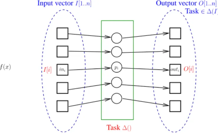
the mapping defining the task. An output value is also called decided value. The way a distributed task extends the notion of a sequential function is described in Figure 1, where the left side represents a classical a sequential function and the right side represents a distributed task.

As in sequential computing (Turing machines) where there are computable functions and uncomputable functions, there are computable tasks and uncomputable tasks. As we will see later write-snapshot and renaming are computable in asynchronous read/write systems despite asynchrony and any number of process failures, while consensus is not [11, 15, 23].

ini pi outi

f

x y= f (x)

Output vectorO[1..n]

Input vectorI[1..n]

Task∈_∆(I)

Task∆()

O[i] I[i]

Functionf()

Figure 1: Function (left) and task (right)

Formal definition A task is a triplehI, O, ∆i where • I is the set of allowed input vectors,

• O is the set of allowed output vectors, and

• ∆ is a mapping of I into O such that (∀I ∈ I) ⇒ (∆(I) ∈ O).

Hence,I[i] and O[i] are the values proposed and decided by pi, respectively, while∆(I) defines the set of output

vectors that can be decided from the input vectorI. (More developments on the definition of tasks and their relation

with topology can be found in [16, 17]).

If one or several processespi, ...,pj, do not participate or crash before deciding an output value, we haveO[i] =

. . . = O[j] = ⊥, and the vector O has then to be such that there is a vector O′ _{∈ ∆(I) that covers O, i.e., (O[i] 6=}

⊥) ⇒ (O′_{[i] = O[i]).}

A simple example: the binary consensus task In this task, a process proposes a value from the set{0, 1}, and all

the non-faulty processes have to decide the same value which has to be a proposed value. LetX0andX1be the vector

of sizen containing only zeros and only ones, respectively.

The setI of input vectors is the set of all the vectors of zeros and ones. The set O of output vectors is {X0, X1}.

Solving a task In the context of this paper, a distributed algorithmA is a set of n local automata (one per process)

that communicate through atomic read/write registers.

The algorithmA solve a task T if, in any run in which each process proposes a value such that the input vector

belongs toI, each non-faulty process decides a value, and the vector O of output values belongs to the set ∆(I).

Tasks vs Objects A task is a mathematical object. From a programming point of view, a concurrent object can be associated with a task (a concurrent object is an object that can be accessed by several processes). Such an object is a one-shot object that provides the processes with a single operation (“one-shot” means that a process can invoke the object operation at most once).

To adopt a more intuitive presentation, the two tasks that are presented below use their object formulation. This formulation expresses the mapping ∆ defining a task by a set of properties that the operation invocations have to

satisfy. These properties can be more restrictive than ∆. This comes from the fact that there is no notion of

time/concurrency/communication pattern in∆, while the set of properties defining the object can implicitly refer

to such notions.

2.3

The write-snapshot task

The write-snapshot task was introduced in [8] (where it is called immediate snapshot). A write-snapshot object pro-vides processes with a single operation denoted write_snapshot(). When a process piinvokes this operation, it

sup-plies as input parameters its identityidiand the value it wants to deposit into the write-snapshot object. Its invocation

returns a setviewicomposed of pairs(idj, vj).

As previously indicated, the specification∆ is expressed here a set of properties that the invocations of write_snapshot()

have to satisfy.

• Self-inclusion. ∀ i: (idi, vi) ∈ viewi.

• Containment. ∀ i, j: (viewi⊆ viewj) ∨ (viewj⊆ viewi).

• Simultaneity.

∀ i, j: [((idj, vj) ∈ viewi) ∧ ((idi, vi) ∈ viewj)] ⇒ (viewi= viewj).

• Termination.

Any invocation of write_snapshot() by a non-faulty process terminates.

A write-snapshot combines in a single operation the write of a value (here a pair(idi, vi)) and a snapshot [1] of

the set of pairs already or concurrently written. Self-inclusion states that a process sees its write. Containment states the views of the pairs deposited are ordered by containment. Simultaneity states that if each of two processes sees the pair deposited by the other one, they have the same view of the deposited pairs. Finally, the termination property states that the progress condition associated with operation invocations is wait-freedom, which means that an invocation by a non-faulty process terminates whatever the behavior of the other processes (which can be slow, crashed, or not participating). An iterative implementation of write-snapshot can be found in [8, 30].

2.4

The adaptive renaming task

This task has been introduced in [3] in the context of asynchronous crash-prone message-passing systems. Thereafter, a lot of renaming algorithms suited to read/write communication have been proposed. An introduction to shared memory renaming, and associated lower bounds, is presented in [9].

While there are onlyn process identities, the space name is usually much bigger than n (as a simple example this

occurs when the name of a machine is the IP address). The aim of the adaptive renaming task is to allow the processes to obtain new names from a new name space which has to depend only on the numberp of processes that want to

obtain a new name (1 ≤ p ≤ n), and be as small as possible. It is shown in [17] that 2p − 1 is a lower bound on the

size of the new name space.

When considering the adaptive renaming task from the point of view of its associated one-shot object, a processpi

that wants to acquire a new name invokes an operation denoted new_name(idi). The set of invocations has to satisfy

the following set of properties.

• Validity. The size of the new name space is 2p − 1. • Agreement. No two processes obtain the same new name.

• Termination.

Any invocation of new_name() by a non-faulty process terminates.

As for the write-snapshot task, the termination property states that a non-faulty process that invokes the operation

new_name() obtains a new name whatever the behavior of the other processes. Agreement states the consistency

condition associated with new names. Validity states the domain of the new names: if a single process wants to obtain a new name, it obtains the name1, if only two processes invoke new_name() they obtain new names in the set {1, 2, 3}, etc. This show that the termination property (wait-freedom progress condition) has a cost in the size of the

new name space: while onlyp new names are needed, the new name space needs (p − 1) additional potential new

names to allow the invocations issued by non-faulty processes to always terminate.

3

A Concurrency-related Recursive Pattern

for Distributed Algorithms

The recursion parameter As already announced, the recursion parameter (denotedx) in the algorithms solving the

tasks we are interested is the number of processes that the invoking process perceives as participating processes. As initially a process has no knowledge of how many processes are participating, it conservatively considers that all other processes participate, and consequently issues a main call witx = n.

Atomic read/write registers and local variables The pattern manages an array SM[n..1], where each SM [x] is a

sub-array of sizen such that SM [x][i] can be written only by pi. A processpistarts executing the recursion levelx by

depositing a value in SM[x][i]. From then on, it is a participating process at level x.

Each process manages locally three variables whose scope is a recursive invocation. smi[n..1] is used to save a

copy of the current value of SM[x][1..n]; partikeeps the number of processes thatpisees as participating at levelx;

andresiis used to save the result returned by the current invocation.

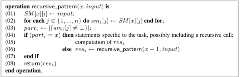
operation recursive_pattern(x, input) is

(01) SM[x][i] ← input;

(02) for each j∈ {1, ..., n} do smi[j] ← SM [x][j] end for;

(03) parti← |{smi[j] 6= ⊥}|;

(04) if(parti= x) then statements specific to the task, possibly including a recursive call;

(05) computation of resi

(06) else resi← recursive_pattern(x − 1, input)

(07) end if

(08) return(resi) end operation.

Figure 2: Concurrency-related recursive pattern

The recursion pattern The generic recursive pattern is described in Figure 2. The invoking processpifirst deposits

its input parameter value in SM[x][i] (line 1), and read the content of the shared memory attached to its recursion level x (line 2). Let us notice that the entries of the array SM [x][1..n] are read in any order and asynchronously. Then, pi

computes the number of processes it sees as participating in the recursion levelx (line 3), and checks if this number is

equal to its current recursion levelx.

• if x = parti (lines 4-5), pi discovers that x processes are involved in the recursion level x. In this case,

it executes statements at the end of which it computes a local result resi. These local statements are

task-dependent and may or not involve a recursive call with recursion levelx − 1.

• if x 6= parti,pi sees less thanx processes participating to the recursion level x. In this case, it invokes the

recursion pattern at levelx − 1 with the same input parameter input, and continues until it attains a recursion

levelx′_{≤ x − 1 at which it sees exactly x}′_{processes that have attained this recursion levelx}′_.

A processpistarts with its recursion parameterx equal n, and then its recursion parameter decreases until the invoking

process returns a result. Hence, a process executes at mostn recursive calls before terminating. The correctness proof

Linear time vs branching time If line 4 does not include a recursive call, the recursive pattern is a linear time pattern. Each participating process executes line 6 until its stops at line 4 (or crashes before). Hence, each process executes a prefix of the same sequence of recursive calls, each with its initial input parameterinput. The algorithm,

whose instantiation from the recursive pattern is described in Section 4, is a linear time implementation of write-snapshot.

If there are recursive calls at line 4, the recursive pattern is a branching time pattern. Such a recursion pattern is characterized by a tree of recursive calls, and a participating process executes a prefix of a single branch of this tree. In this case, each SM[x] is composed of several sub-arrays, each of them being an array of n SWMR atomic

registers. The algorithm, whose instantiation from the recursive pattern is described in Section 5, is a branching time implementation of renaming.

4

Linear Time Recursion

4.1

A recursive write-snapshot algorithm

An instantiation of the recursive pattern which implements write-snapshot is described in Figure 3. This recursive implementation has been introduced in [13], and the representation adopted here is from [30]. This instantiation is nearly the same as the original recursive pattern. More precisely, the input parameterinput of a process piis the pair

(idi, vi).

The line numbering is the same as in the recursive pattern. As there is no specific statement to instantiate at line 4 of the recursive pattern, its lines 4 and 5 are instantiated by a single line denoted 4+5.

A processpiinvokes first write_snapshot(n, (idi, vi)) where viis the value it wants to deposit in the write-snapshot

object.

operation write_snapshot(x, (idi, vi)) is

(1) SM[x][i] ← (idi, vi);

(2) for each j∈ {1, ..., n} do smi[j] ← SM [x][j] end for;

(3) parti← |{smi[j] 6= ⊥}|;

(4+5) if(parti= x) then resi← {smi[j] 6= ⊥}

(6) else resi← write_snapshot(x − 1, (idi, vi))

(7) end if

(8) return(resi) end operation.

Figure 3: A recursive write-snapshot algorithm [13]

As already said, the recursion of this algorithm is a linear time recursion. This appears clearly from the arrays of atomic read/write registers accessed by the recursive calls issued by the processes: each process accesses first SM[n],

then SM[n − 1], etc., until it stops at SM [x] where n ≥ x ≥ 1.

4.2

Proof of the algorithm

Theorem 1 [13] The algorithm described in Figure 3 implements a write-snapshot object. For a processpi, The

step complexity (number of shared memory accesses) for a processpiisO(n(n − |resi| + 1)), where resiis the set

returned by the invocation of write_snapshot() issued by pi.

Proof This proof is from [30]. While a process terminates an invocation when it executes the return() statement at

line 8, we say that it terminates at line 4+5 or line 6, according to the line where the returned valueresi has been

computed.

Claim C. If at mostx processes invoke write_snapshot(x, −), (a) at most (x−1) processes invoke write_snapshot(x− 1, −), and (b) at least one process stops at line 4+5 of its invocation of write_snapshot(x, −).

Proof of claim C. Assuming that at mostx processes invoke write_snapshot(x, −), let pkbe the last process that writes

into SM[x][1..n] (as the registers are atomic, the notion of “last” is well-defined). We necessarily have partk ≤ x. If

pkfindspartk = x, it stops at line 4+5. Otherwise, we have partk < x and pkinvokes write_snapshot(x − 1, −) at

that fewer than x processes have written into SM [x][1..n], and consequently, at most (x − 1) processes invoke write_snapshot(x − 1, −). End of the proof of claim C.

To prove termination, let us consider a non-faulty processpithat invokes write_snapshot(n, −). It follows from

Claim C and the fact that at mostn processes invoke write_snapshot(n, −) that either pistops at that invocation or

belongs to the set of at most(n − 1) processes that invoke write_snapshot(n − 1, −). It then follows, by

induc-tion from the claim C, that if pi has not stopped during a previous invocation, it is the only process that invokes

write_snapshot(1, −). It then follows from the text of the algorithm that it stops at that invocation.

The proof of the self-inclusion property is trivial. Before stopping at recursion levelx (line 4+5), a process pihas

writtenviinto SM[x][i] (line 1), and consequently we have then (idi, vi) ∈ viewi, which concludes the proof of the

self-inclusion property.

To prove the self-containment and simultaneity properties, let us first consider the case of two processes that return at the same recursion levelx. If a process pi returns at line 4+5 of recursion levelx, let resi[x] denote the

corresponding value ofresi. Among the processes that stop at recursion levelx, let pibe the last process which writes

into SM[x][1..n]. As pistops, this means that SM[x][1..n] has exactly x entries different from ⊥ and (due to Claim

C) no more of its entries will be set to a non-⊥ value. It follows that, as any other process pj that stops at recursion

levelx reads x non-⊥ entries from SM [x][1..n], we have resi[x] = resj[x] which proves the properties.

Let us now consider the case of two processes pi andpj that return at line 6 of recursion level x and y,

re-spectively, withx > y (i.e., pi returnsresi[x] while pj returnsresj[y]). The self-containment follows then from

x > y and the fact that pjhas written into all the arrays SM[z][1..n] with n ≥ z ≥ y, from which we conclude that

resj[y] ⊆ resi[x]. Moreover, as x > y, pihas not written into SM[y][1..n] while pjhas written into SM[x][1..n], and

consequently(idj, vj) ∈ resi[x] while (idi, vi) /∈ resj[y], from which both he containment and immediacy properties

follow.

As far as the number of shared memory accesses is concerned we have the following. Let res be the set returned by an invocation of write_snapshot(n, −). Each recursive invocation costs n + 1 shared memory accesses (lines 1

and 2). Moreover, the sequence of invocations, namely write_snapshot(n, −), write_snapshot(n − 1, −), etc., until write_snapshot(|res|, −) (where x = |res| is the recursion level at which the recursion stops) contains n − |res| + 1

invocations. It follows that the step complexity for a processpiisO(n(n − |resi| + 1)) accesses to atomic registers.

2T heorem 1

4.3

Example of an execution

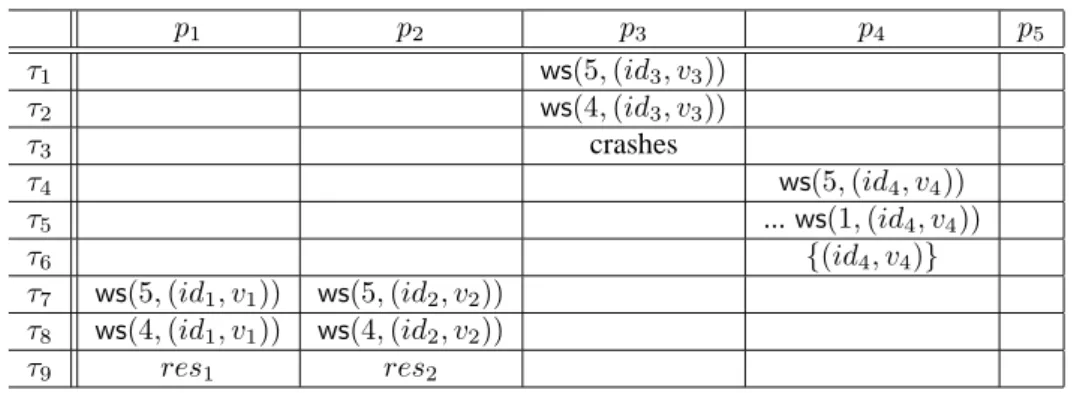
This section described simple executions wheren = 5 and process p5crashes before taking any step (or –equivalently–

does not participate). These executions are described in Table 1 and Table 2. In these tables write_snapshot() is

abbreviated as ws(). p1 p2 p3 p4 p5 τ1 ws(5, (id3, v3)) τ2 ws(4, (id3, v3)) τ3 crashes τ4 ws(5, (id4, v4)) τ5 ... ws(1, (id4, v4)) τ6 {(id4, v4)} τ7 ws(5, (id1, v1)) ws(5, (id2, v2)) τ8 ws(4, (id1, v1)) ws(4, (id2, v2)) τ9 res1 res2

A first execution

1. At timeτ1,p3invokes write_snapshot(5, (id3, v3)). This triggers at time τ2the recursive invocation write_snapshot(4, (id3, v3))

Then,p3crashes after it has writtenid3into SM[4][3] at time τ3.

2. At a later time τ4, p4 invokes write_snapshot(5, (id4, v4)), which recursively ends up with the invocation

write_snapshot(1, (id4, v4)) at time τ5, and consequently p4 returns the singleton set{id4, v4)} at time τ6.

3. At timeτ7, processesp1andp4start executing synchronously:p1invokes write_snapshot(5, (id1, v1)), while p2

invokes write_snapshot(5, (id2, v2)), which entails at time τ8–always synchronously– the recursive invocations

write_snapshot(4, (id1, v1)) and write_snapshot(4, (id2, v2)). As SM [4] contains four non-⊥ entries, both p1

andp2returnsres1andres2which are such thatres1= res2= {(id1, v1), (id2, v2), (id3, v3), (id3, v4)}.

p1 p2 p3 p4 p5

τ10 ws(3, (id3, v3))

τ11 ws(2, (id3, v3))

τ12 res3

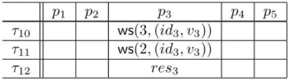
Table 2: Write-snapshot execution: continuing the example

Continuing the example Let us assume that instead of crashing at timeτ3,p3paused for an arbitrary long period

starting after it has read SM[4][1..5] (hence it has seen only two non-⊥ values in SM [4]).

1. At timeτ10,p3wakes up and, aspart3 6= 4, it it issues the recursive invocation write_snapshot(3, (id3, v3)),

which entails at timeτ11the invocation write_snapshot(2, (id3, v3)).

2. As at timeτ12, the shared array SM[2] contains two non-⊥ values, process p4returnsres3= {(id3, v3), (id3, v4)}.

The reader can check that, if before pausing at timeτ3,p3has read only SM[4][4] and SM [4][5], it will read the

other entries SM[4][1], SM [4][2], and SM [4][3], when it wakes up, and its invocation write_snapshot(4, (id3, v3))

will stop the recursion and returnres3= res1= res2.

5

Branching Time Recursion

5.1

A recursive renaming algorithm

An instance of the recursive pattern implementing adaptive renaming is described in Figure 4. This recursive imple-mentation, inspired from the sketch of an algorithm skeleton succinctly described in [13], has been introduced in [27], where it is proved correct. As for the previous recursive algorithm, the representation adopted here is from [30]. The core of this recursive algorithm is the instantiation of line 4 of the recursive pattern, where appears branching time recursion.

Underlying idea: the case of two processes The base case is whenn = 2. A process pifirst writes its identityidi

in the shared memory, and then reads the content of the memory.

• If, according to what it has read from the shared memory, a process sees only itself, it adopt the new name 1. • Otherwise it knows its identity and the one of the other process (idj). It then compares its identityidiandidj,

and does the following: ifidi> idj, it adopts the new name 3, ifidi< idj, it adopts the new name 2.

The new name space is consequently[1..2p − 1] where p (number of participating processes) is 1 or 2.

The underlying shared memory The shared memory SM[n..1] accessed by processes is now a three-dimensional

array SM[n..1, 1..2n − 1, {up, down}] such that SM [x , first , dir ] is a an array of n atomic read/write registers. SM[x , first , dir ][i] can be written only by pibut can be read by all processes.

When more than two processes participate The algorithm is described in Figure 4. A process invokes first

new_name(n, 1, up, idi). It then recursively invokes new_name(x, 1, up, idi), until the recursion level x is equal

to the number of processes thatpisees as competing for a new name.

As we are about to see, given a pair(first , dir ), the algorithm ensures that at most x processes invoke new_name(x , first , dir , −).

These processes compete for new names in a space name of size2x − 1 which is the interval [first..first + (2x − 2)]

ifdir = up, and [first − (2x − 2)..first] if dir = down. Hence, the value up is used to indicate that the concerned

processes are renaming “from left to right” (as far as the new names are concerned), whiledown is used to indicate

that the concerned processes are renaming “from right to left” (this is developed below when explaining the splitter behavior of the underlying read/write registers.) Hence, a processpiconsiders initially the renaming space[1..2n − 1],

and then (as farpiis concerned) this space will shrink at each recursive invocation (going up or going down) untilpi

obtains a new name.

operation new_name(x , first, dir , idi) is

(1) SM[x , first, dir ][i] ← idi;

(2) for each j∈ {1, ..., n} do smi[j] ← SM [x, first, dir ][j] end for;

(3) parti← |{smi[j] 6= ⊥}|;

(4+5).1 if(parti= x) then last ← first = dir (2x − 2 );

(4+5).2 if(idi= max(smi)

(4+5).3 then resi← last

(4+5).4 else resi← new_name(x − 1, last + dir, dir, idi))

(4+5).5 end if

(6) else resi← new_name(x − 1, first, dir , idi))

(7) end if

(8) return(resi) end operation.

Figure 4: A recursive adaptive renaming algorithm [13]

The recursive algorithm The lines 1-3 and 6-8 are the same as in the recursive pattern where SM[x] is replaced by SM[x, first, dir]. The lines which are specific to adaptive renaming are the statements in the then part of the recursive

pattern (lines 4-5). These statements are instantiated by the new lines (4+5).1-(4+5).5, which constitute an appropriate instantiation suited adaptive renaming.

For each triple(x, f, d), all invocations new_name(−, x, f , d) coordinate their respective behavior with the help

of the sizen array of atomic read/write registers SM [x, f, d][1..n]. At line (4+5).”, max(smi) denotes the greatest

pro-cess identity present insmi. As a processpideposits its identity in SM[x, first , dir][i] before reading SM [x, first, dir][1..n],

it follows thatsmicontains at least one process identity when read bypi.

Let us observe that, if onlyp processes invoke new_name(n, 1, up, −), p < n, then all of them will invoke the

algo-rithm recursively, first with new_name(n − 1, 1, up), then new_name(n − 2, 1, up), etc., until new_name(p, 1, up, −).

Only at this point, the behavior of a participating processpidepend on the concurrency pattern (namely, it may or may

not invoke the algorithm recursively, and with eitherup or down).

Splitter behavior associated with SM[x, first , dir] (The notion of a splitter has been informally introduced in [21].)

Considering the (at most)x processes that invoke new_name(x, first, dir, −), the splitter behavior associated with the

array of atomic registers SM[x, first , dir] is defined by the following properties. Let x′ _{= x − 1.}

• At most x′_{= x − 1 processes invoke new_name(x − 1, first, dir, −) (line 6. Hence, these processes will obtain}

new names in an interval of size(2x′_{− 1) as follows:}

– Ifdir = up, the new names will be in the “going up” interval [first..first + (2x′_{− 2)],}

– Ifdir = down, the new names will be in the “going down” interval [first − (2x′_{− 2)..first].}

• At most x′ _{= x − 1 processes invoke new_name(x − 1, last + dir, dir) (line (4 5).4), where last = first +}

dir(2x − 2) (line (4 5).1). Hence, these x′_{= x − 1 processes will obtain their new names in a renaming space}

of size(2x′_{− 1) starting at last + 1 and going from left to right if dir = up, or starting at last − 1 and going}

from right to left if dir = down. Let us observe that the value last ± 1 is considered as the starting name

because the slot last is reserved for the new name of the process (if any) that stops during its invocation of

• At most one process “stops”, i.e., defines its new name as last = first + dir(2x − 2) (lines (4 5).2 and (4 5.3).

Let us observe that the only processpkthat can stop is the one such thatidk has the greatest value in the array

SM[x, first , dir][1..n] which contains then exactly x identities.

5.2

Example of an execution

A proof of the previous algorithm can be found in [30]. This section presents an example of an execution of this algorithm. It considers four processesp1,p2,p3, andp4.

First: processp3executes alone Processp3invokes new_name(4, 1, up, id1) while (for the moment) no other

pro-cess invokes the renaming operation. It follows from the algorithm thatp3invokes recursively new_name(3, 1, up, id1),

then new_name(2, 1, up, id1), and finally new_name(1, 1, up, id1). During the last invocation, it obtains the new

name1. This is illustrated in Figure 5. As, during its execution, p3sees onlyp = 1 process (namely, itself), it decides

consistently in the new name space[1..2p − 1] = 1.

p3obtains the new name1

it decides the new name2p − 1 =1 As p3has seen p= 1 process (itself)

SM_{[4, 1, up]}

p3invokes new_name(4, 1, up, id3)

p3invokes new_name(2, 1, up, id3)

p3invokes new_name(3, 1, up, id3)

p3invokes new_name(1, 1, up, id3)

p1and p4invoke concurrently new_name(4, 1, up, −)

After p3has obtained the new name1

which entail their concurrent invocations of new_name(3, 1, up, −)

Figure 5: Recursive renaming: first,p3executes alone

Then: processesp1andp4invoke new_name() After p3has obtained a new name, bothp1andp4invoke new_name(4, 1, up, −)

(See Figure 6). As they see only three processes that have written their identities into SM[4, 1, up], both concurrently

invoke new_name(3, 1, up, −) and consequently both compute last = 1 + (2 ∗ 3 − 2) = 5. Hence their new name

space is[1..5].

Now, let us assume thatp1stops executing whilep4executes alone. Moreover, letid1, id4 < id3. As it has not

the greatest identity among the processes that have accessed SM[3, 1, up] (namely, the processes p1,p3andp4),p4

invokes first new_name(2, 4, down, id4) and then recursively new_name(1, 4, down, id4), and finally obtains the new

name4.

After processp4has obtained its new name,p1continues its execution, invokes new_name(2, 4, down, id1) and

computeslast = 4 − (2 × 2 − 2) = 2. The behavior of p1depends then on the values ofid1andid4. Ifid4< id1,

p1decides the namelast = 4 − (2 × 2 − 2) = 2. If id4> id1,p1invokes new_name(1, 3, 1, id1) and finally decides

the name3.

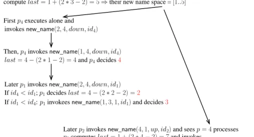
Finally, if laterp2invokes new_name(4, 1, up, id2), it sees that the splitter SM [4, 1, up] was accessed by four

new_name(2, 6, down, id1), new_name(1, 6, down, id1), at the end of which it computes last == 6+(2×1−2) = −

and decides the name6.

The multiplicity of branching times appears clearly on this example. As an example, the branch of time ex-perienced byp3(which is represented by the sequence of accesses to SM[4, 1, up], SM [3, 1, up], SM [2, 1, up], and

SM[1, 1, up]), is different from the branch of time experienced by p4(which is represented by the sequence of accesses

to SM[4, 1, up], SM [3, 1, up], SM [2, 4, down], and SM [1, 4, up]).

First p4executes alone and

compute last= 1 + (2 ∗ 3 − 2) = 5 ⇒ their new name space = [1..5]

last= 4 − (2 ∗ 1 − 2) = 4 and p4decides4

Let id1, id4< id3

If id4< id1; p1decides last= 4 − (2 ∗ 2 − 2) =2

p1and p4invoke new_name(3, 1, up, −), they see p = 3 processes and both

invokes new_name(2, 4, down, id4)

Then, p4invokes new_name(1, 4, down, id4)

Later p1invokes new_name(2, 4, down, id1)

If id1< id4: p1invokees new_name(1, 3, 1, id1) and decides3

p2computes last= 1 + (2 ∗ 4 − 2) = 7 and invokes

new_name(3, 6, −1, id₂), new_name(2, 6, −1, id₂), new_name(1, 6, −1, id₂) p2then computes last= 6 − (2 ∗ 1 − 2) = 6 and decides6

Later p2invokes new_name(4, 1, up, id2) and sees p = 4 processes

Figure 6: Recursive renaming:p1andp4invoke new_name(4, 1, up, −)

Let us observe that the new name space attributed to thep = 3 processes p1,p3, andp4(the only ones that, up to

now, have invoked new_name(4, 1, up)()) is [1..2p − 1] = [1..5].

Finally processp2invokes new_name() Let us now assume thatp2invokes new_name(4, 1, up, id2). Moreover, let

id2< id − 1, id2, id3. Processp2sees thatp = 4 processes have accessed the splitter SM [4, 1, up], and consequently

computeslast = 1 + (2 × 4 − 2) = 7. The size of its new name space is [1..2p − 1] = [1..7]. As it does

not have the greatest initial name among the four processes,p2invokes new_name(3, 6, down, id2), and recursively

new_name(2, 6, down) and new_name(1, 6, down, id − 2), and finally obtains 6 as its new name.

6

Conclusion

The aim of this paper is to be an introductory tutorial on concurrency-related recursion in asynchronous read/write systems where any number of processes may crash. The paper has shown that a new type of recursion is introduced by the net effect of asynchrony and failures, namely the recursion parameter is used to allow a process to learn the number of processes with which it has to coordinate to compute its local result. This recursion has been illustrated with two task examples, write-snapshot and adaptive renaming. Interestingly, the first example is related to a linear time notion, while the second one is related to a branching time notion.

Acknowledgments

A special acknowledgment to E. Gafni, whose seminal work on recursive distributed renaming contributed to this presentation.

References

[1] Afek Y., Attiya H., Dolev D., Gafni E., Merritt M. and Shavit N., Atomic snapshots of shared memory. Journal of the ACM, 40(4):873-890, 1993.

[2] Akl S.G., The design and analysis of parallel algorithms. Prentice-Hall Int’l Series, 401 pages, 1989.

[3] Attiya H., Bar-Noy A., Dolev D., Peleg D. and Reischuk R., Renaming in an asynchronous environment. Journal of the ACM, 37(3):524-548, 1990.

[4] Attiya H., Fouren A., and Gafni E., An adaptive collect algorithm with applications. Distributed Computing, 15(2): 87-96, 2002.

[5] Attiya H., Herlihy M. and Rachman O., Atomic snapshots using lattice agreement. Distributed Computing, 8(3):121-132, 1995.

[6] Attiya H. and Welch J.L., Distributed computing: fundamentals, simulations and advanced topics, (2d Edition), Wiley-Interscience, 414 pages, 2004 (ISBN 0-471-45324-2).

[7] Bar-Noy A., Dolev D., Dwork C. and Strong R., Shifting gears: changing algorithms on the fly to expedite Byzantine agreement. Information and Computation, 97(2):205-233, 1992.

[8] Borowsky E. and Gafni E., Immediate atomic snapshots and fast renaming. Proc. 12th ACM Symposium on Principles of Distributed Computing (PODC’93), pp. 41-51, 1993.

[9] Castañeda, Rajsbaum S., and Raynal M., The renaming problem in shared memory systems: An introduction. Computer Science Review, 5(3):229-251, 2011.

[10] Dahl O.J., Dijkstra E.W., and Hoare C.A.R., Structured programming. Academic Press, 220 pages, 1972 (ISBN 0-12-200550-3).

[11] Fischer M.J., Lynch N.A., and Paterson M.S., Impossibility of distributed consensus with one faulty process. Journal of the ACM, 32(2):374-382, 1985.

[12] Francez N., Hailpern B., and Taubendfeld G., Script: a communication abstraction mechanism and its verification. Science of Computer Programming, 6:35-88, 1986.

[13] Gafni E. and Rajsbaum S., Recursion in distributed computing. Proc. 12th Int’l l Symposium on Stabilization, Safety, and Security of Distributed Systems (SSS ’10), Springer LNCS 6366, pp. 362-376, 2010.

[14] Harel D. and Feldman Y., Algorithmics: the spirit of computing (third edition). Springer, 572 pages, 2012 (ISBN 978-3-642-27265-3).

[15] Herlihy M.P., Wait-free synchronization. ACM Transactions on Programming Languages and Systems, 13(1):124-149, 1991. [16] Herlihy M.P., Rajsbaum S., and Raynal M., Power and limits of distributed computing shared memory models. To appear

Theoretical Computer Science, (http://dx.doi.org/10.1016/j.tcs.2013.03.002), 2013.

[17] Herlihy M.P. and Shavit N., The topological structure of asynchronous computability. Journal ACM, 46(6):858-923, 1999. [18] Herlihy M.P. and Wing J.M, Linearizability: a correctness condition for concurrent objects. ACM Transactions on

Program-ming Languages and Systems, 12(3):463-492, 1990.

[19] Horowitz E. and Shani S., Fundamentals of computer algorithms. Pitman, 626 pages, 1978 (ISBN 0-273-01324-0).

[20] Lamport. L., On Interprocess Communication, Part 1: Basic formalism, Part II: Algorithms. Distributed Computing, 1(2):77-101,1986.

[21] Lamport L., Fast mutual exclusion. ACM Transactions on Computer Systems, 5(1):1-11, 1987.

[22] Lamport L., Shostak E., and Pease M.C., The Byzantine general problem. ACM Transactions on Programming Languages and Systems, 4(3):382-401, 1982.

[23] Loui M. and Abu-Amara H., Memory requirements for agreement among unreliable asynchronous processes. Advances in Computing Research, 4:163-183, JAI Press, 1987.

[24] Lynch N.A., Distributed Algorithms. Morgan Kaufmann Pub., San Francisco (CA), 872 pages, 1996.

[25] Mehlhorn K. and Sanders P., Algorithms and data structures. Springer, 300 pages, 2008 (ISBN 978-3-540-77977-3). [26] Onofre J.-C., Rajsbaum S., and Raynal M., A topological perspective of recursion in distributed computing. Tech report,

UNAM (Mexico), 12 pages, 2013.

[27] Rajsbaum S. and Raynal M., A theory-oriented introduction to wait-free synchronization based on the adaptive renaming problem. Proc. 25th Int’l Conference on Advanced Information Networking and Applications (AINA’11), IEEE Press, pp. 356-363, 2011.

[28] Randell B., Recursively structured distributed computing systems. Proc. 3rd Symposium on Reliability in Distributed Software and Database Systems, IEEE Press, pp. 3-11, 1983.

[29] Raynal M., Fault-tolerant agreement in synchronous distributed systems. Morgan & Claypool, 167 pages, 2010 (ISBN 978-1-608-45525-6).

[30] Raynal M., Concurrent programming: algorithms, principles and foundations. Springer, 515 pages, 2013 (ISBN 978-3-642-32026-2).