HAL Id: hal-02474779
https://hal-ifp.archives-ouvertes.fr/hal-02474779
Preprint submitted on 27 Feb 2020
HAL is a multi-disciplinary open access archive for the deposit and dissemination of sci-entific research documents, whether they are pub-lished or not. The documents may come from teaching and research institutions in France or abroad, or from public or private research centers.
L’archive ouverte pluridisciplinaire HAL, est destinée au dépôt et à la diffusion de documents scientifiques de niveau recherche, publiés ou non, émanant des établissements d’enseignement et de recherche français ou étrangers, des laboratoires publics ou privés.
Personal car, public transport and other alternatives?
Predicting potential modal shifts from multinomial logit
models and bootstrap confidence intervals
Amandine Chevalier, Frédéric Lantz
To cite this version:
Amandine Chevalier, Frédéric Lantz. Personal car, public transport and other alternatives? Predicting potential modal shifts from multinomial logit models and bootstrap confidence intervals: Cahiers de l’Economie, Série Recherche, n° 91. 2013. �hal-02474779�
IFP Energies nouvelles - IFP School - Centre Économie et Gestion 228-232, av. Napoléon Bonaparte, F-92852 Rueil-Malmaison Cedex, FRANCE
Personal car, public transport and other
alternatives?
Predicting potential modal shifts from
multinomial logit models and bootstrap
confidence intervals
Amandine CHEVALIER
Frédéric LANTZ
Novembre 2013
Les cahiers de l'économie - n° 91
Série Recherche
amandine_chevalier@hotmail.fr frederic.lantz@ifpen.fr
La collection "Les cahiers de l’économie" a pour objectif de présenter des travaux réalisés à IFP Energies nouvelles et à IFP School, travaux de recherche ou notes de synthèse en économie, finance et gestion. La forme
peut être encore provisoire, afin de susciter des échanges de points de vue sur les sujets abordés. Les opinions émises dans les textes publiés dans cette collection doivent être considérées comme propres à leurs auteurs et
ne reflètent pas nécessairement le point de vue d’ IFP Energies nouvelles ou d' IFP School.
Pour toute information sur le contenu, prière de contacter directement l'auteur.
Pour toute information complémentaire, prière de contacter le Centre Économie et Gestion: Tél +33 1 47 52 72 27
The views expressed in this paper are those of the authors and do not imply endorsement by the IFP Energies Nouvelles or the IFP School. Neither these institutions nor the authors accept any liability for loss or
2
Personal car, public transport and other alternatives? Predicting
potential modal shifts from multinomial logit models and
bootstrap confidence intervals
Amandine Chevalier
a,b,c,1, Frédéric Lantz
baBIPE, Issy-les-Moulineaux, France bIFPEN, Rueil-Malmaison, France cCERNA, Mines ParisTech, Paris, France
Abstract
Households’ daily mobility in France is characterized by the preponderance of the automobile. Passenger cars, mainly used by households but not only, are thus responsible for more than a half of fuel consumptions in road transport (CGDD/SOeS, July 2013) and more than a half of CO2 emissions in the
transport sector (SOeS/CDC, December 2012). The main objective of this paper is thus to explain the modal choice of French households for their daily trips, particularly the importance of the car, and to predict potential shifts from personal car to public transport and other alternatives, especially shared car. An independent multinomial logit model is estimated and reveals the particular importance of car equipment on modal choices and specifically on car use. Predictions by 2020 are conducted according to three cases for the household’s motorization (no car, one car, two cars or more) and per different mobility profiles. Personal car should remain the main mode of transportation by 2020 except if households have no car. In that case, modal shares would be more balanced, public transport would become the main transport mode and the shift to shared car would be at a maximum. Modal share of shared car could thus reach 16% for “exclusive motorists”. A conditional logit model is also estimated and shows no particular importance of the means of transportation’s costs in the modal choices. These results show that the increase in distances between 2010 and 2020 makes motorized modes more necessary. Thus, personal car and public transport should remain the main modes of transportation by 2020. Moreover, expected changes in costs and travel time by 2020 does not seem to have any effect on the deployment of shared car, its modal share being constant (in an average) between 2010 and 2020.
Keywords: Modal choice; personal car; public transport; shared car; multinomial logit model; conditional
logit model; bootstrap confidence intervals.
3 Introduction
Households’ daily mobility in France is characterized by the preponderance of the automobile. Passenger cars, mainly used by households but not only, are thus responsible for more than a half of fuel consumptions in road transport (CGDD/SOeS, July 2013) and more than a half of CO2 emissions in the transport sector (SOeS/CDC,
December 2012). But in recent years, we observe a decrease in fuel consumptions by private cars and an increase of fuel consumptions by motorcycles and buses and coaches (CPDP, 2012), suggesting a modal shift from private car to motorcycles and public transport. In the same time indeed, inflections in car use are observed. Thus, young people use less private car and are less often motorized than their elders. Moreover, households try to adapt to the high cost of car by travelling less kilometers by car each year, by pooling its use thanks to new mobility services such as carpooling and carsharing and by using more public transport in urban area.
The new mobility services, especially carsharing, can be considered as empirical applications of the business model of the functional service economy. According to some researchers, the new business model consisting of the substitution of the sale of the product’s function to the sale of its property, which is the concept behind the new individual mobility services we mentioned, allows for a decrease in production, lower consumption of natural resources, in addition to encouraging companies to design products that consume fewer resources in their production, use, maintenance, recycling and reuse (Bourg and Buclet, 2005; Du Tertre, 2007). Fourcroy and Chevalier (2012) show that great energy savings can be achieved by these services only if they replace car ownership and do not add a new need of car.
Moreover, compared to the use of private car by only one person, the use of public transport allows for a decrease in energy consumptions and CO2 emissions per capita.
These are the reasons why the main objective of this paper is to explain the modal choice of French households for their daily trips, particularly the importance of the car, to predict potential shifts from personal car to alternatives such as public transport, motorcycle or shared car.
From survey data (Mobility Observatory, BIPE, October 2010), we base on households’ activities, ie their need for mobility, their car equipment, and socio-economic variables that could impact their modal choices. We estimate an independent multinomial logit model from these variables and a conditional logit model from characteristics of each mean of transportation (cost and travel time). From these estimations, we simulate modal choices by 2020 and apply a pairs bootstrap method to predict modal shares with confidence intervals.
In a first part of the paper, we present a brief review of the literature. Then we describe the method and the data we use in this paper. Our results are then presented. The fourth section is devoted to the predictions of modal shares by 2020 and the last section to the discussion of our results.
1. Literature review
The decision of an individual among several unordered alternatives is generally modelled through multinomial logit models. As an example of such a decision, the choice between means of transport is modelled in this way. Modal choice models such as those estimated by Train (1977), Carson et al. (1994) and more recently Hensher (2008) are mainly built from quantitative data describing the characteristics of the various modes (costs, transfer or transport time, etc.). They can then be used to test the effects of a transport policy (construction of a new road, creation of a new line of transport, etc.). Thus, from a sample interviewed before the introduction of the Bay Area Rapid Transit (BART) in San Francisco in 1973, Train (1977) developed a model to measure the effect of the service in terms of modal split. From the same type of model, Carson et al. (1994) wanted to know how can change the modal share of the car if its cost increases. More generally, research on modal choices show that they are influenced by the level of service (travel time and cost differentials), but also by the characteristics of individuals and households, such as the level of income, car equipment, area of residence and place of work (Stopher and Meyberg 1975, Koppelman and Pas, 1980 Kanafani, 1983, Ben-Akiva and Lerman, 1985; Wachs, 1991). Moreover, the choice of a mode of transportation can be studied for a particular type of trip, most often commuting. This is particularly what study Train (1977) in San Francisco, Hensher (2008) in six Australian cities, Liu (2007) in Shanghai, Khattak and Palma in Brussels (1997).
Some are also interested in the impact of unexpected events on the modal choice. Thus, Khattak and Le Colletter (1994), and Khattak et al. (1995) show that longer travel time on road may encourage motorists to use public transport. Moreover, Khattak and Palma (1997) show that adverse weather conditions encourage half of motorists in Brussels to change their departure time or their itinerary.
It can also be question of interdependence between the choice of transport mode and trip purpose, more precisely the organization of trips depending on the schedule of the day. Thus one part of the literature focuses on modal choices on the basis of household’s activities (activity-based demand model). Damm (1983), Golob and Golob (1983), Kitamura (1988) and Etterna (1996) conduct literature reviews on this subject. We mainly retain that Pas
4
(1984) shows that demographic factors such as employment status, gender, or the presence of children in the household have a significant impact on the activities and trips. In addition, Kitamura (1984) identifies the interdependence between the choice of destinations in travel chains and the choice of the mode of transportation. Moreover, Bhat and Koppelman (1993) propose an analytical model based on the organization of activities. More specifically and always on the basis of households’ activities, the first models of travel chains were mainly developed in the 70’s and 80’s in the Netherlands (Daly et al, 1983; Gunn et al, 1987; Hague Consulting Group, 1992; Gunn, 1994). They were then used to model the movements in different cities and countries: Stockholm (Algers et al, 1995), Salerno, Italy (Cascetta et al, 1993), Boise, Idaho (Shiftan, 1995), New Hampshire (Rossi and Shiftan, 1997) or Boston (Bowman and Ben-Akiva, 2000). A key finding highlighted by Krygsman et al. (2007) is that there are variations in the order of choice of travel mode and trip purpose. But in most cases, the travel pattern is done before the modal choice. This therefore indicates that it rather depends on the choice of the pattern and the travel chain considered. It is precisely on this need for mobility we base to try to explain the modal choice, as well as on variables describing individuals and households and variables that are characteristics of the different modal choices (travel costs and time).
2. Methodology and data
As described in the introduction, the decrease in fuel consumptions by private cars and the increase of fuel consumptions by motorcycles and buses and coaches observed in recent years (figure 1), suggest a modal shift from private cars to motorcycles and public transport. Moreover, we observe a shared use of the car especially through carpooling and carsharing. Thus we decide to explain the modal choice of French households to predict potential shifts from personal cars to alternatives such as public transport, motorcycles or shared cars by 2020. The transport mode’s choice is based on several factors corresponding to the travel mode’s (distance, time, etc.) and to the household’s characteristics. As mentioned in the previous section, there is a large literature on this topic. Each study point out that the choices are related to the characteristics of a country at a given period. A classical way to assess these choices is to use a multinomial logit model which aims to explain the modal choices by a set of explanatory factors. In the next two paragraphs, we develop the econometric approach that we use for the models’ estimations and forecasts. Then, we present the data which are considered for the statistical estimation.
2.1. Multinomial logit model
The objective of the model is to explain that each individual i (i,=1,…n) has a choice between a set of unordered alternatives j (j=0,…m). Here, we consider m+1=6 alternative transportation’s modes.As this dependent variable is a qualitative one with a limited number of unordered terms, we use a discrete choice model: the multinomial logit model (MLN).
More specifically, we use two types of logit models: single or independent multinomial and conditional. The distinction between these two types of models is primarily based on the nature of the selected explanatory variables. The first includes variables that are characteristics of individuals, while the second includes variables that are characteristics of the different means of transportation and differ according to the dependent variables and individuals as well. In the case of modal choice, individual i compares the different levels of utility associated with different choices and chooses the one that maximizes his utility from the j choices.
Figure 1 – Fuel consumption in France (a) in 2000 and (b) 2011, from CPDP (2012) 0,2 23,0 6,5 8,5 0,7 3,5 Motorcycles Private cars Light trucks Heavy trucks Buses and coaches Others 0,6 22,4 7,2 5,8 0,9 4,2
5 For individual i, the utility of the choice j is:
Uij =f ( β Xij)+ εij (1)
Where β is a vector of unknown parameters, Xij is a vector of the individuals’ or households’ characteristics and
εij a random error term.
As MLN are probabilistic models, their results reflect the utility maximization. Thus the probability that the individual i chooses the alternative j is the probability that the value of j is greater than that associated with all other modes. For instance, for j=0:
Prob(yi=0)=Prob (Ui0 > Ui1, Ui0 > Ui2,… Ui0 > Uim ) (2)
We denote Uij = Vij + εij where Vij is a deterministic function and εij a random variable.
Thus, the probability that the individual i chooses the alternative 0 is:
Prob(yi=0) = 𝑒 𝑣𝑖𝑗
∑𝑚𝑘=1𝑒𝑣𝑖𝑘 (3)
As Vij = xiβj, in the case of an independent logit model, then the probability that the individual i chooses the
alternative j is: Prob(yi=0) = 𝑒 𝑥𝑖𝛽𝑗 1+ ∑𝑚 𝑒𝑥𝑖𝛽𝑘 𝑘=1 (4)
As Vij = xijβ, in the case of a conditional logit model, then the probability that the individual i chooses the
alternative j is:
Prob(yi=0) = 𝑒 𝛽𝑧∗𝑖𝑗
1+ ∑𝑚𝑘=1𝑒𝛽𝑧∗𝑖𝑘 (5)
Where z*i,j = xi,k – xi,0
The parameters’ estimations are obtained by the method of maximizing the log likelihood of the model with constants using the SAS software version 9.4 through Logistic and Mdc procedures.
2.2. Bootstrap prediction intervals
The estimated multinomial logit models are then used for predictions. For this purpose, we consider a set of expected future values of the explanatory variables Xf from which we predict the probability of each
transportation’s mode Prob(yf=j).
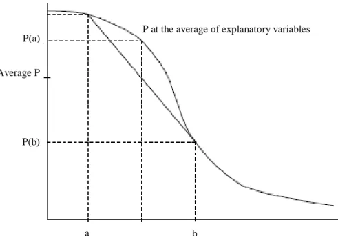
From logit model, it is only possible to perform predictions for ‘‘case study’’ i.e. for a new individual representative of the population in 2020. Thus, we set the main explanatory variables according to their most probable evolution by 2020 in an average. However, the probability distribution being not linear, the average probabilities predicted by the models are not equal to the probability at the average of the variables as shown in figure 2. It is therefore imperative to provide predictions with confidence intervals. To do this, we use the method of bootstrap prediction intervals.
The principle of the bootstrap is to approximate the theoretical distribution of a statistic of interest from the empirical distribution obtained from B random samples of size N in the sample of the original data. In our case, we repeat B=1,000 times a random drawing with replacement of 1,413 individuals of the original population with their characteristics (pairs bootstrap) to get 1,000 bootstrap samples. We then estimate the models on each of the 1,000 samples to obtain an empirical distribution of the probabilities predicted by the models.
From these distributions we construct confidence intervals with 95% degree of confidence.
6
Figure 2 – Theoretical probability distribution of predicted probabilities
2.3. Data and economic analysis
As described in the literature review, modal choices are associated with travel needs corresponding to the distance to travel for different purposes, individuals’ characteristics, and travel cost and time. The assessment of these choices depends therefore on individual data based on surveys. In our case, we base on a sample of 1,413 people (representative of the French population) involved in the Mobility Observatory (BIPE, October 2010). This survey is conducted every six months to describe mobility practices of French households. The questionnaire is passed face to face during 45 minutes to one hour. For this work, we take into account three main questions concerning the travel modes used for a “normal week day”, the transportation mode used for the different mobility patterns and the distance travelled with each of the different travel mode. Thus we define travel needs as the distance to travel for each of the mobility purpose.
The variable to explain is the modal choice on a normal week day. We take into account the primary mode of transportation that is the one with which individual travel the highest distance each day. It has six categories: personal car (including company car), shared car (carpooling and carsharing), motorcycle, bike, walking and public transport. The modal distribution of the sample is described in figure 3. 59% of individuals use personal car which is the main mode of transportation to travel each day. Thus 84% of daily kilometres are travelled by personal car. The second mode is public transport used by 20% of the sample to travel 12% of the travel needs each day, followed by walking for 15%. Shared car is used by only 1% (homogeneous groups of people for carpooling and carsharing) to travel less than 1% of the daily travel needs.
In a preliminary work on the same data set we performed a multiple correspondence analysis from the main individuals’ socio-economic and travel characteristics (see table 1 in appendix). It shows that the most discriminating variables distinguishing mobility profiles are: the travel need, i.e. the distance to travel (in km / pattern), the type of the municipality of residence (density), the marital status, the household’s motorization, the age, the employment status and the income. Thus we use these variables to estimate multinomial logit models to explain modal choice. Moreover, this work led to the construction of mobility profiles described in figure 4.
a b
P at the average of explanatory variables
Average P
P(b) P(a)
7
Figure 3 – Modal distribution of the sample (a) among individuals and (b) passenger-kilometers (Mobility Observatory, BIPE, October, 2010)
The first level of partition distinguishes “exclusive motorists” from others. These individuals have the highest travel needs for all patterns and move exclusively by car. They are from 30 to 60, are working, live in couple and have children. They live in low density areas and are motorized. The rest of the population is then cut in two classes: people using their car (exclusively or in combination with one or more other modes) and people being “multimodal”. The third level of partition occurs between individuals using the car (the “motorists”), some travelling on low distances, others having higher travel needs and living in lower density areas. Within the group of “multimodal” we then distinguish people living alone (rather non-working or workers, under 30 or over 60, without children, with modest incomes, living in large city-center, non-motorized and travelling mainly by motorcycle, walking and public transport), from people living in family (with two working persons, under 60, with children, living in Paris area and large city-center, motorized and travelling mainly by car, motorcycle, walking or public transport). Within the “singles” we distinguish “pensioners” of more than 60, living alone and walking or using public transport, from “young” inactive or low-skilled labour, living alone or with roommates, and travelling mainly by motorcycle, walking or public transport. Finally, within the “families” we distinguish “working couples” of more than 30 and travelling mainly by car, from “students” of less than 30 travelling mainly by motorcycle, walking or public transport.
Finally we select the following explanatory variables to explain modal choices for daily trips: the travel need which corresponds to the distance to travel for different purposes and is linked to the density of the municipality of residence (from 1=Paris to 7=rural area), the household’s motorization (0 car, 1 car, 2 cars or more) which is linked to the household’s income, the marital status (single, couples, cohabitation / roommate) and the age linked to the employment status (0=not working, 1= working).
Multimodal Single Family Motorists Pensioners walking and using public transport 12% Working and motorist couples 23% Students alternative to car 4% Travel on low distances 15% Travel on medium distances 16% Exclusive motorists travelling on high distances 12% Young alternative to car 20%
Figure 4 – Mobility profiles
84% 1% 1% 1% 2% 12% 59% 1% 3% 3% 15% 20% Personal car Shared car Motorcycle Bike Walking Public transport
8
In addition, it is possible to model modal choices from their own characteristics: their costs and travel time. The expenditure incurred by the travellers to the use of public transport in France was calculated by the National Federation of Transport Users (FNAUT, 2012) and corresponds to the price paid by users for public transport thus taking into account state aids. The costs of personal car and motorcycle correspond to the mileage rates set by the French tax administration. The cost of shared car is a half of that of the private car.
The travel time with each mode of transport is also taken into account to explain modal choice. It is calculated from the distance to travel and the average speed associated with each of the transportation mode (the average speed is that observed in the Mobility Observatory in October 2010).
3. Results
From the different characteristics we thus estimate two types of logit models: an independent model from individuals’ characteristics and a conditional model from the travel modes’ characteristics.
3.1. Independent logit model 3.1.1. Estimated parameters
We estimate an independent multinomial logit model explaining the modal choice between six different modes (personal car, shared car, motorcycle, bike, walking and public transport) by the explanatory variables distance to travel, density of the municipality of residence, household’s motorization, age, marital status, employment status and income. The distance is the log of the kilometers travelled each day with the primary transportation mode, the density of the municipality of residence is a density index going from 1 for Paris to 7 for the rural area, the household’s motorization corresponds to three cases: the household has no car, one car, or two cars or more, the marital status as well: single, in couple, or in cohabitation, and the employment status is a binary variable: 0 if the person is not working and 1 if the person is working.
Quality indicators of the model are good enough (ρ² McFadden: 0.58 and Estrella indicator: 0.95), but the estimators associated with activity status and income are not significant so we cannot say that they have an effect on the modal split in the sample we study. This conclusion cannot be generalized to the total population in that the significance of the parameters depends on the sample size. We decide anyway to remove the employment status and income variables, which does not deteriorate the quality of the model in so far as the employment status is clearly correlated to the age and the income to the household’s motorization. This one is therefore an indicator of standard of living. The model is estimated with the personal car as the reference.
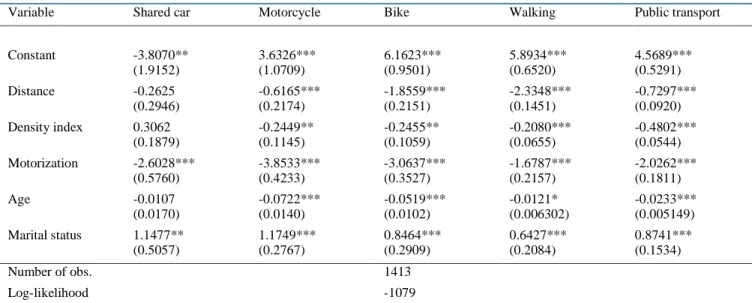
Table 1 shows that the distance has a negative effect on the use of alternatives to the personal car: the longer the distance to travel, the greater the probability to choose the personal car. Similarly, the lower the density of the residence area, the higher the household is motorized, the older the person and the more there are people in the household, and the more the alternatives to the car are used.
Table 1 – Estimated parameters
Variable Shared car Motorcycle Bike Walking Public transport
Constant -3.8070** (1.9152) 3.6326*** (1.0709) 6.1623*** (0.9501) 5.8934*** (0.6520) 4.5689*** (0.5291) Distance -0.2625 (0.2946) -0.6165*** (0.2174) -1.8559*** (0.2151) -2.3348*** (0.1451) -0.7297*** (0.0920) Density index 0.3062 (0.1879) -0.2449** (0.1145) -0.2455** (0.1059) -0.2080*** (0.0655) -0.4802*** (0.0544) Motorization -2.6028*** (0.5760) -3.8533*** (0.4233) -3.0637*** (0.3527) -1.6787*** (0.2157) -2.0262*** (0.1811) Age -0.0107 (0.0170) -0.0722*** (0.0140) -0.0519*** (0.0102) -0.0121* (0.006302) -0.0233*** (0.005149) Marital status 1.1477** (0.5057) 1.1749*** (0.2767) 0.8464*** (0.2909) 0.6427*** (0.2084) 0.8741*** (0.1534) Number of obs. 1413 Log-likelihood -1079
Standard deviation in parenthesis
9
Only variables of motorization and marital status appear to have an effect on the choice between personal and shared car. Obviously, non-motorized people have no choice than using shared car. Contrary to intuition, age does not seem to have any effect on the choice between personal car and shared car. In addition, motorization seems to be crucial. However, it is important to remain vigilant with these findings in that, on the observed sample, we have very few individuals using shared car.
3.1.2. Odds ratio
The interpretation of estimated parameters can be specified by measuring the magnitude of a change in explanatory variables on the probability to use each mode of transportation through odds ratio presented in table 2.
Odds ratios are calculated as follows:
Odds ratio kj = exp [βkj] (6)
Table 2 – Odds ratio
Variable Shared car Motorcycle Bike Walking Public transport
Distance 0.769 0.540 0.156 0.097 0.482
Density index 1.358 0.783 0.782 0.812 0.619
Motorization 0.074 0.021 0.047 0.187 0.132
Age 0.989 0.930 0.949 0.988 0.977
Marital status 3.151 3.238 2.331 1.902 2.397
Increasing the distance to travel of one unit decreases the probability of using alternative modes to personal car of 0.23 points (1-0.769) for shared car, 0.46 points for motorcycle, 0.84 points for bike, 0.90 points for walking and 0.52 points for public transport. Concerning shared car, this result shows that for a given level of distance to travel, it is better to own a private car than sharing a car when needed so that individuals are quite rational.
Similarly, the decrease in the density of the residential area decreases the same probability from 0.38 points for public transport to 0.19 for walking, but increases the probability to use shared car, which means that it should rather develop in low density areas. But we must be careful with this conclusion which is mainly explained by the fact that shared car is mainly used in the less dense area in our sample.
To be older of one year also decreases this probability: from 0.07 points for motorcycle to 0.01 points for shared car.
An extra car owned by the household also decreases this probability: from 0.98 points for motorcycle to 0.81 points for walking. The motorization is crucial: its effect on the probability of choosing the different modes of transportation is the largest. Once purchased, the car is thus used almost exclusively. This conclusion has been already widely demonstrated in the literature.
Finally, with an additional person in the household, it is 1.9 times more likely to choose walking than personal car or 3.24 times more likely to choose motorcycle. Thus, the more in the household (even if it is motorized), the less likely to use the personal car.
3.1.3. Independence of Irrelevant Alternatives (IIA) assumption test
To test the independence of irrelevant alternatives assumption necessary to validate the multinomial logit model, we realize the test proposed by Hausman and McFadden (1984). Thus, we calculate the test statistic S for five different sub-groups in which we removed each time a modality (except personal car which is the reference category). Thus we consider A1 the sub-group excluding shared car, A2 excluding motorcycle, A3 excluding bike,
A4 excluding walking and A5 excluding public transport.
As shown by Hausman and McFadden (1984), the test statistic can be negative, especially in the case of small samples. This does not then challenge the IIA property. As shown in table 3, in the case of subgroups excluding motorcycle, walking and public transport, the test statistic S follows a 𝜒² distribution with 24 degrees of freedom. In the subgroup excluding motorcycle, the test statistic is less than the critical value (at 99.5%) so we do not reject H0. P-value = 1 also tells us that there are 100% chance of being wrong in rejecting the null hypothesis of
independence. The IIA assumption is indeed satisfied in this case. Similarly, in the subgroup excluding walking, the test statistic is less than the critical value (at 99.5%) so we do not reject H0, p-value = 0.99 also indicates that
there are 99% chance of being wrong in rejecting the null hypothesis of independence. Finally, in the subgroup excluding public transport, p-value = 0.87 indicates that there are 87% chance of being wrong in rejecting the null
10
hypothesis. Thus we do not reject the null hypothesis at 87% and have 13% chance that our model does not respect this property.
Table 3 – Results of the IIA assumption test
S p-value
A1 : shared car excluded Negative
A2 : motorcycle excluded 2.6645332 1.00
A3 : bike excluded Negative
A4 : walking excluded 6.0857236 0.99
A5 : public transport excluded 16.570484 0.87
3.2. Conditional logit model
To take into account the economic rationality of individuals in their modal choices, we estimate a conditional logit model, taking into account variables that are characteristics of choices: the cost and travel time. In addition, we also introduce specific constants for each mode of transport to take into account their own characteristics hardly captured elsewhere (including comfort for example).
Table 4 shows that parameters associated with the constants are all negative which confirms the preference for personal car compared to all other means of transportation for its comfort, flexibility… In addition, the parameters associated with the cost and travel time are negative which means that a high cost and a long travel time do not encourage the use of alternative modes to the personal car. This result shows that mobility is an arbitrable need on the basis of its cost. Thus, odds ratios show that an increase in the cost of a transport mode (of a cent per kilometer) decreases by 0.02 points the probability of its use (1-0998). Similarly, an increase in the travel time of one minute of a mode of transport decreases by 0.06 points the probability of its use.
The model is estimated with the personal car as the reference.
Table 4 – Conditional logit model: estimated parameters and odds ratio
Variable Estimated parameters Odds ratio
Cs_shared car -4.2787*** (0.2931) 0.014 Cs_motorcycle -3.1629*** (0.1711) 0.042 Cs_bike -2.6704*** (0.1585) 0.069 Cs_walking -0.4331*** (0.1155) 0.649 Cs-public transport -0.9830*** (0.0710) 0.374 Cost -0.0016** (0.0008) 0.998 Travel time -0.0055*** (0.0007) 0.994 Number of observations 1414 Log-likelihood -1573 ρ² McFadden 37.89 Estrella indicator 81.57
Standard deviation in parenthesis
11 4. Predictions by 2020 and bootstrap prediction intervals
The objective of the predictions is to predict the modal choices in 2020 from the estimated models. Thus we set the main explanatory variables according to their most probable evolution, in an average, by 2020 to try to approach the closest to reality.
4.1. Independent logit model 4.1.1. Hypothesis
The independent logit model explaining modal choices is estimated using the following variables: the distance, the category of the municipality of residence (density), age, motorization and marital status.
About the distance to travel, we base on figures from the National Transportation Survey (INSEE, 1982; INSEE, 1994; SOeS, 2008) to realize a projection to 2020 based on a logarithmic adjustment on previous data and continuing the observed trend. Indeed, according to a recent report to the French Minister of Transport by the Commission “Mobilité 21” (2013), travel need should grow by 2020 but its growth should be weaker than in the past. These evolutions are applied to the data in our sample. Therefore, the log of the distance to travel in 2010 was 3.029 and will be 3.102 in 2020. This result is that applying on an average of the sample, but the trend between 2010 and 2020 is applied to the average distances observed in each subgroup used to perform predictions (different mobility profiles) and that is the case for all other explanatory variables.
In our sample, the mean age is 47.2 years in 2010. According to population’s projections made by the BIPE (Residential Migration, 2010), the average age is expected to increase in 2020 and should be 48.7 years.
In our sample, people living in a couple are the majority. According to the BIPE’s projections (Residential Migration, 2010), this mode of cohabitation should remain dominant in 2020 but the number of households of one person is expected to grow: singles will be 45% of the households in 2020 (42% in 2010) and couples will be 52% (55% in 2010).
Concerning the evolution of the distribution of households between urban and rural areas, projections of the BIPE (Residential Migration, 2010) show no significant changes by 2020. Therefore, we do not change the structure depending on the category of municipality of residence.
Finally, as motorization is a key explanatory variable of modal choice, we perform predictions in three cases: the household has no car, the household has one car (current situation on average and therefore central scenario) and the household has two cars or more.
4.1.2. Predictions and bootstrap confidence intervals
To obtain results close from reality, we realize our forecasts according to the different mobility profiles presented in section 2.3 (figure 3). From the logit model we obtain the choice probability of the average individual representative of each profile. Moreover, we consider three sets of values for explanatory variables according to the households’ motorization (no car, one car, two cars or more).
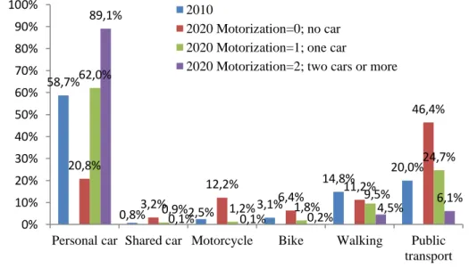
Figure 5 – Modal shares in France in 2010 and 2020 according to three cases of motorization
58,7% 0,8% 2,5% 3,1% 14,8% 20,0% 20,8% 3,2% 12,2% 6,4% 11,2% 46,4% 62,0% 0,9% 1,2% 1,8% 9,5% 24,7% 89,1% 0,1% 0,1% 0,2% 4,5% 6,1% 0% 10% 20% 30% 40% 50% 60% 70% 80% 90% 100%
Personal car Shared car Motorcycle Bike Walking Public transport 2010
2020 Motorization=0; no car 2020 Motorization=1; one car
12
The aggregated results correspond to the weighted sum of the average individual forecasts for each mobility profile as recommended by Ben-Akiva & Lerman (1985). They provide the modal split described in the figure 5. In the original sample, 18% of households are not motorized, 62% have one car and 20% have two cars or more. The results show a wide variation depending on the motorization scenario. Personal car should remain the main mode of transportation by 2020 except if households have no car. In that case, public transport would become the main mode of transportation, the modal distribution would be more balanced and shared car would deploy. More specifically, these general conclusions should be specified by discussing the results per mobility profile.
We choose to provide the detailed results of two extreme profiles, the others being just discussed.
The “pensioners walking and using public transport” mainly includes people with no car. That is why we study only one alternative: the equipment (one car), as shown in table 5. In this case, the probability of using the private car increases while that of all other modes decreases. Being by nature not very motorists “pensioners walking and public transport” do not constitute an important target for car-sharing: 2.37% at a maximum as shown by bootstrap confidence intervals.
Table 5 – Modal shares of “pensioners walking and using public transport” in 2010 and 2020
Year Personal car Shared car Motorcycle Bike Walking Public
transport 2010 observed 26.38% 1.84% 0% 3.07% 35.58% 33.13% 2020 No car 16.43% 1.12% 1.49% 7.3% 42.9% 30.76% Bootstrap confidence intervals 95% [12.53 ; 20.94] [0.19 ; 2.37] [0.53 ; 2.8] [3.75 ; 10.7] [35.82 ; 50.1] [24.89 ; 37.66]
Similarly “young alternative to car” use less car (personal and shared) than the average population and more motorcycle, bike and public transport. They are mainly motorized (one car). The shared car could only grow in the case of a household with no car to 3.93% at a maximum.
“Working and motorist couples” however use more personal car than the average population and are an attractive target for car-sharing, especially in the case of a household without a car. In that scenario the use of public transport could also develop significantly, especially since they mainly live in urban areas (Paris and its region and city centers of more than 100,000 inhabitants).
“Students alternative to car” mainly use public transport and motorcycle. They are also the second shared car users. But their low car use (personal as shared) does not make them a prime target for shared car. Thus, a decrease in the use of personal car is accompanied by an increase of motorcycle, bike and walking.
“Motorists” on the contrary use more personal car than the average population. The more their travel needs are important, the more they use it. They are preferred targets for car-sharing, but also for motorcycle and public transport, primarily in a scenario of a household not motorized.
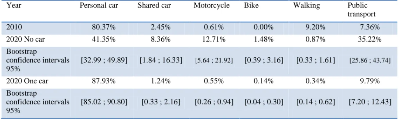
Table 6 – Modal shares of “exclusive motorists travelling on high distances” in 2010 and 2020
Year Personal car Shared car Motorcycle Bike Walking Public
transport 2010 80.37% 2.45% 0.61% 0.00% 9.20% 7.36% 2020 No car 41.35% 8.36% 12.71% 1.48% 0.87% 35.22% Bootstrap confidence intervals 95% [32.99 ; 49.89] [1.84 ; 16.33] [5.64 ; 21.92] [0.39 ; 3.16] [0.33 ; 1.61] [25.86 ; 43.74] 2020 One car 87.93% 1.24% 0.55% 0.14% 0.34% 9.79% Bootstrap confidence intervals 95% [85.02 ; 90.80] [0.33 ; 2.16] [0.26 ; 0.94] [0.04 ; 0.30] [0.14 ; 0.62] [7.20 ; 12.43]
“Exclusive motorists travelling on high distances” (table 6) are the first users of shared cars and the main target for developing its use for daily trips. This share could even reach 16% of the modal share of this mobility profile. But even in that case, shared car would not become the main mode of transportation, which would remain personal
13
car (obviously company car) and public transport would represent a third of modal shares. Motorcycle would also develop substantially.
4.1.3. Substitutions between travel modes
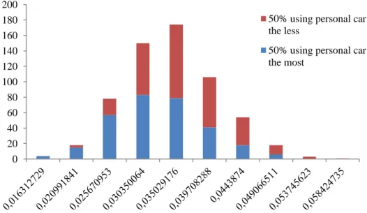
From bootstrap replications, we obtain statistical distributions of probabilities predicted by the independent model. In the case where the household has no car, we study potential modal shifts from personal car to public transport, motorcycle and shared car by distinguishing the probabilities to use them depending on whether we are above or below the median of the probability of using private car.
As shown by figures 6, 7 and 8, the people using the less personal car (the 50% using personal car the less) are more among those using public transport, motorcycle and shared car the most. Thus we observe a potential modal shift from personal car to public transport, motorcycle or shared car.
Figure 6 – Statistical distribution of predicted probabilities for public transport by 2020
Figure 7 – Statistical distribution of predicted probabilities for motorcycle by 2020
0 20 40 60 80 100 120 140 160 180
50% using personal car the less
50% using personal car the most
14
Figure 8 – Statistical distribution of predicted probabilities for shared car by 2020
4.2. Conditional logit model 4.2.1. Hypothesis
The conditional model is estimated from the variables of cost and travel time.
Concerning transportation costs, we base on the calculation of expenses incurred by the travellers by car and public transport between 1970 and 2010 conducted by the National Federation of Transport Users (2012). In 2020, these costs correspond to the projection of the linear fit of the observed costs between 1970 and 2010. This evolution is then applied to the cost of other modes of transportation (shared car and motorcycle). The transportation costs to 2020 will therefore continue to increase.
In addition, we propose a scenario in which we apply a carbon tax. Indeed, at the environmental conference on 20 and 21 September 2013, the entry into force of a Climate-Energy Contribution (CEC) in 2014 was announced (Le Figaro, September 20th, 2013). The price of a ton of carbon is 7 € in 2014 and then increases to 14.5€ in 2015 and
22 € in 2016. In 2020, we retain a CO2 price at 22 € / ton. At this price, the impact of the tax on the user cost per
kilometer of the car or motorcycle is almost zero (0.4 € cents / km). We also apply very high taxes but no inflection in use behaviour of different modes of transport is observed.
Finally, the transport time to 2020 depends on the evolution of distances whose assumptions were presented in section 4.1.1, the speed remaining constant. Therefore, the average transport time will increase by 6% by car and motorcycle, 6.7% by bike, 7.6% by walking and 8.1% by public transport.
4.2.2. Predictions and bootstrap confidence intervals
The predictions are performed at the average point of the sample and give the modal distribution shown in figure 9. These results show that the increase in distances between 2010 and 2020 makes motorized modes more necessary. Thus, personal car and public transport should remain the main modes of transportation by 2020. In addition, costs of the different means of transport increasing linearly, differentials of cost do not vary. Arbitrations are thus rather realised in terms of travel time than costs.
Concerning shard car more precisely, expected changes in costs and travel time by 2020 does not seem to have any effect on its deployment, its modal share being constant (in an average) between 2010 and 2020. It will be 1.21% at a maximum as shown in table 7.
Predictions have also been realized taking into account a carbon tax. At different prices of the carbon tax (from 22€/ton to very high taxes), costs do not really differ from the situation without a carbon tax and no modal shift is observed. Moreover, even if the car costs are doubled, we do not observe modal shifts or a significant increase in the use of shared car.
0 20 40 60 80 100 120 140 160 180 200
50% using personal car the less
50% using personal car the most
15
Figure 9 – Modal shares in France in 2010 and 2020
Table 7 – Modal shares in France and bootstrap confidence intervals in 2010 and 2020
Year Personal car Shared car Motorcycle Bike Walking Public
transport
2010 58,7% 0,8% 2,5% 3,1% 15,0% 20,0%
2020 60,0% 0,8% 2,6% 3,4% 12,1% 21,2%
Bootstrap CI [57,25 ; 67,25] [0,45 ; 1,21] [1,87 ; 3,34] [2,57 ; 4,15] [0,39 ; 15,39] [19,00 ; 26,18]
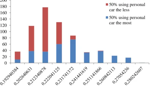
4.2.3. Substitutions between travel modes
From bootstrap replications, we obtain statistical distributions of probabilities predicted by the conditional model. Thus we study potential modal shifts from personal car to public transport, motorcycle and shared car with the same method than in the section 4.1.3.
Figure 10 – Statistical distribution of predicted probabilities for public transport by 2020
58,7% 0,8% 2,5% 3,1% 15,0% 20,0% 60,0% 0,8% 2,6% 3,4% 12,1% 21,2% 0% 10% 20% 30% 40% 50% 60% 70%
Personal car Shared car Motorcycle Bike Walking Public transport 2010 2020 0 20 40 60 80 100 120 140 160 180 200 50% using personal car the less
50% using personal car the most
16
Figure 11 – Statistical distribution of predicted probabilities for motorcycle by 2020
Figure 12 – Statistical distribution of predicted probabilities for shared car by 2020
As shown by figures 10, 11 and 12, the people using the less personal car use public transport and motorcycle the less too and shared car the most. From rational considerations, we observe less modal shifts from personal car to public transport or motorcycle but rather to shared car.
5. Discussion
Firstly, conclusions have to be taken with caution, especially for shared car, because we do not dispose of a large sample to analyze travel behavior and there are few observations concerning the use of shared car for daily trips. However, this is the only French survey representative of the French population and taking into account shared
0 20 40 60 80 100 120 140
160 50% using personal car
the less
50% using personal car the most
17
car as a daily travel mode. The Household Travel Surveys only concern urban areas and the National Transportation Survey does not take into account shared car (carpooling and carsharing) as a daily travel mode. From the independent logit model, predictions by 2020 have been conducted by mobility profiles to reflect the diversity of mobility habits. However, application of these mobility profiles to the conditional logit model does not allow assessing correctly the modal distribution observed in 2010. As a consequence, predictions from the conditional logit model have been performed at the average point. That means that, apart from purely rational considerations (cost and time of transport), modal choices are driven by other factors that are characteristics of households and their travel needs. Those two approaches are thus complementary and show that personal car should remain the main mean of transportation by 2020 with public transport.
Predictions by 2020 have been performed according to three cases of household’s motorization from the independent logit model. We show that the use of personal car could decrease only if household’s motorization decreases. In that case public transport would become the main mode of transportation and shared car would develop. But this situation of household’s de-motorization is obviously not possible by 2020. However, changes in households’ motorization are observed and it will be determinant to work on the future of households’ motorization to know precisely its future level. Moreover, we notice that, even for a household with no car, modal share of personal car is not zero. This is explained by the fact that we introduce company car as a personal car in so far the household has it at its disposal as a private car owned by the household. In 2010, 2.6% of the sample use company car as a daily travel mode. The predictions results by 2020 show that personal car’s share could reach 20% in the case of not motorized households. That means that there always will be a need of car available to households but that the mode of holding will change: the car will not necessarily owned by the household. Thus personal car and public transport should remain the main modes of transportation by 2020, which implies that the supply of them should be available and sufficient everywhere.
In addition, forecasts from the conditional logit model could be achieved by income deciles to highlight the weight of the transport budget (as shown by Merceron and Theuliere, 2010) and the implications of a potential carbon tax on households more or less wealthy and dependent on their car that is hidden by the prediction from a midpoint. Finally, methods used in this paper to measure the potential development of shared cars in daily trips do not take into account diffusion phenomena or learning effects. Predictions realized in this paper are thus floor values for the use of shared car by 2020.
6. Conclusion
This paper shows that the main drivers of modal choices are the distance to travel, the density, the age, the marital status, the household’s motorization, and travel cost and time. In an independent multinomial logit model, we confirm that motorization is the most determining factor of modal choices of French households in general and car use in particular. Thus the results of predictions by 2020 show a wide variation depending on the motorization scenario. In addition, the longer the distance to travel, the more we use motorized modes. However, an increase in the distance to travel results in a decrease of the probability to use shared car. This probably means that people with the highest needs to travel are motorized (what is then more profitable than carsharing) and suggests that shared car can hardly become a mean of transportation used exclusively. Thus the predictions show that personal car should remain the main mode of transportation by 2020, except if households have no car, which is the only case in which shared car could deploy, but in which public transport would become the main mode of transportation with personal car and motorcycle. Moreover, the study of statistical distributions of predicted probabilities for public transport, motorcycles and shared cars shows a substitution from personal car to these alternative travel modes. Furthermore, “motorists” are the main target for shared car, which means that we could observe shift from personal to shared car. But “motorists” are also those with the highest travel needs and the most motorized. In addition, the estimation of a conditional logit model based on variables characteristics of the different modes of transportation (travel cost and time) shows that economic rationality explains modal choices as well and that the two approaches are complementary. Moreover, the increase in distances between 2010 and 2020 makes motorized modes more necessary. Thus, personal car and public transport should remain the main modes of transportation by 2020. Furthermore, only very high values of carbon tax could influence modal choices. However, expected changes in costs and travel time by 2020 does not seem to have any effect on the deployment of shared car, its modal share being constant (in an average) between 2010 and 2020. It could be 1.21% at a maximum. But from rational considerations, we observe less potential modal shifts from personal car to public transport and motorcycles but rather to shared cars. Therefore, the use of shared car seems to correspond to a specific profile and be essentially driven by the motorization of the households (as for all other travel modes). But the relationship between motorization and shared car use is not very simple and the de-motorization of households is not really possible by 2020, that is the reason why it will be determinant to work on the future of households’ motorization and to connect the results with the predictions realized in this paper
18 Acknowledgment
The authors would like to thanks particularly Leopold Simar, Fanny Rougier, Hugo Delavaquerie and Simon Michaut for their help at different steps of this work.
References
Algers, S., Daly, A., Kjellman, P., Widlert, S., (1995). Stockholm model system (SIMS): application. In: Seventh World Conference of Transportation Research. Sydney, Australia.
Ben-Akiva, M., & Lerman, S. R. (1985). Discrete Choice Analysis: Theory and Application to Travel Demand. Cambridge: MIT Press. 384 p.
Bhat, C., & Koppelman, F. S. (1993). A conceptual framework of individual activity program generation.
Transportation Research, 27A (6), 433-446.
BIPE (November 2010). Mobility Observatory. Confidential documentation BIPE (2010). Residential Migration. Confidential documentation
Bourg, D., & Buclet, N. (2005). Des services aux entreprises à l’économie de la fonctionnalité : les enjeux du développement durable, Futuribles, 313, 27-37.
Bowman, J.L., & Ben-Akiva, M.E. (2000). Activity-based disaggregate travel demand model system with activity schedule. Transportation Research, Part A, 35, 1-28
Carson, R.T. et al. (1994). Experimental analysis of choice. Maketing Letters, 5:4, 351-368.
Cascetta, E., Nuzzolo, A., Velardi, V. (1993). A system of mathematical models for the evaluation of integrated trac planning and control policies. Unpublished Research Paper, Laboratorio Richerche Gestione e Controllo Traco, Salerno, Italy.
CGDD/SoES (July, 2013). Les comptes des transports en 2012, Références. 166 p.
Commission « Mobilité 21 » (27th June, 2013). Pour un schéma national de mobilité durable, Rapport au ministre
chargé des transports, de la mer et de la pêche. 91 p. CPDP (2012). Pétrole 2012. CPDP. 325 p
Daly, A.J., van Zwam, H.H.P., van der Valk, J. (1983). Application of disaggregate models for a regional transport study in The Netherlands. In: World Conference on Transport Research. Hamburg.
Damm, D. (1983). Theory and empirical results: a comparison of recent activity-based research. In: S. Carpenter, & P. Jones (Eds.), Recent Advances in Travel Demand Analysis (pp.3-33). London: Gower.
Du Tertre, C. (2007). L'économie de fonctionnalité. Changer la consommation dans le sens du développement durable. In E. Heurgon, & J. Landrieu, L’économie des services pour un développement durable. Nouvelles
richesses, nouvelles solidarité, Colloque de Cerisy, Prospective, Essais et Recherche, Paris: l’Harmattan. 390 p.
Efron, B., & Tibshirani, R. J. (1994). An introduction to the bootstrap. Monographs on statistics and applied probability 57, Chapman & Hall. 456 p.
Ettema, D. (1996). Activity-based travel demand modeling. Ph.D. Thesis, Technische Universiteit Eindhoven, The Netherlands.
Fédération National des Associations d’Usagers des Transports (2102). Dépenses engagées par les voyageurs : comparaison entre les transports publics et la voiture particulière. Tours. 52 p.
Fourcroy, C., & Chevalier A. (2012). Functional service economy: a pathway to real energy savings? The case of vehicle rental by French households. In: International Society for Ecological Economics Conference 2012, Rio de Jainero, Brazil.
19
Golob, J. M., & Golob, T.F. (1983). A classification of approaches to travel-behavior analysis. Special Report 201, Transportation Research Board, Washington, DC. 115 p.
Gunn, H. (1994). The Netherlands National Model: a review of seven years of application. International
Transactions in Operational Research 1 (2), 125-133.
Gunn, H.F., van der Hoorn, A.I.J.M., Daly, A.J. (1987). Long range country-wide travel demand forecasts from models of individual choice. In: Fifth International Conference on Travel Behaviour. 1987, Aix-en Provence, France.
Hague Consulting Group (1992). The Netherlands National Model 1990: The National Model System for Travel and Transport. Ministry of Transport and Public Works, The Netherlands.
Hausman, J., & McFadden D. (1984). Specification Tests for the Multinomial Logit Model. Econometrica, 52, n°5, 1219-1240.
Hensher, D.A. (2008). Empirical approach to combining revealed and stated preference data: some recent developments with reference to urban mode choice. Research in Transportation Economics, 23, 23-29. INSEE. (1982). Transport 1981-1982. Centre Maurice Halbwachs.
INSEE. (1994). Transports et communications 1993-1994. Centre Maurice Halbwachs. Kanafani, A. (1983). Transportation Demand Analysis. New York:.McGraw Hill. 320 p.
Khattak, A. & Le Colletter, E. (1994). Stated and Reported Diversion to Public Transportation under Incident Conditions: Implications on the Benefits of Multimodal ATIS, Partners in Advanced Transit and Highways (PATH) Research Report UCB-ITS-PRR-94-14. Institute of Transportation Studies, University of California at Berkeley, California, Presented at the 4th Annual Meeting of IVHS America, Atlanta, Georgia.
Khattak, A., Polydoropoulou, A. and Ben-Akiva, M. (1995). Commuters’ normal and shift decisions in unexpected congestion: Pre-trip response to advanced traveler information systems, Presented at the 74th Annual Meeting of the Transportation Research Board, Preprint No. 950990, Washington, D.C. Transportation Research Record, 1537. Transportation Research Board, Washington, DC. 46-54
Khattak, A. & De Palma, A., (1997). The impact of adverse weather conditions on the propensity to change travel decisions: a survey of Brussels commuters. Transportation Research Part A, 31, 181-203
Kitamura, R. (1984). Incorporating trip chaining into analysis of destination choice. Transportation Research B, 18B (4), 67-81.
Kitamura, R. (1988). An evaluation of activity-based travel analysis. Transportation, 15, 9-34.
Koppelman, F., & Pas, E. (1980). Travel-choice Behavior: Models of Perceptions, Feelings, Preference, and Choice. Transportation Research Record, 765, 26-33.
Krygsman S., Arentz T., & Timmermans H. (2007). Capturing tour mode and activity choice interdependencies: A co-evolutionaly logit modelling approach. Transportation Research, 41A, 913-933.
Liu, G. (2008), A behavioral model of work-trip mode choice in Shanghai. China Economic Review, 18, 456-476 Merceron, S., & Theuliere, M. (October 2010). Les dépenses d’énergie des ménages depuis 20 ans : une part en moyenne stable dans le budget, des inégalités acccrues. INSEE Première, n°1315. 4 p.
Nodé-Langlois, F. (September, 20th, 2013). Hollande confirme la création d’une taxe carbone. Lefigaro.fr
Pas, E.I. (1984). The effect of selected socio-demographic characteristics on daily travel-activity behaviour.
20
Rossi, T.F. & Shiftan, Y. (1997). Tour Based Travel Demand Modeling in the US. In: Eighth Symposium on Transportation Systems. Ghania, Greece, 40-414.
Shiftan, Y. (1995). A practical approach to incorporate trip chaining in urban travel models. In: Fifth National Conference on Transportation Planning Methods and Applications. Seattle, Washington.
SOeS (2008). Transports et déplacements (ENTD) 2008. Centre Maurice Halbwachs. SOeS, CDC (2012). Chiffres clés du climat France et monde, Edition 2013. Repères, 48 p.
Stopher, P., & Meyberg, A. (1975). Urban Transportation Modelling and Planning. Lexington Books, Lexington D.C. Mass. 345 p.
Train, K. (1977). A validation test of a disaggregate mode choice model. Transportation Research, 12, 167-174. Wachs, M. (1991). Policy implications of recent behavioral research in transportation demand management.
21 Appendix
Table of variables used for multiple correspondence analysis
Variable Label Description N
Travel mode
Mod1 Car only 840 (55.4%)
Mod2 Motorcycle 34 (2.2%)
Mod3 Bike 43 (2.8%)
Mod4 Walking 141 (9.3%)
Mod5 Public transport 64 (4.2%)
Mod6 Walking+public transport 162 (10.7%)
Mod7 Car+walking 127 (8.4%)
Mod8 Car+others 104 (6.9%)
Sex homm Male 719 (47.4%)
femm Female 797 (52.6%) Age age1 < 30 278 (18.3%) age2 30-39 277 (18.3%) age3 40-49 283 (18.7%) age4 50-59 249 (16.4%) age5 60-69 276 (18.2%) age6 >69 50 (3.3%) Marital status Celi Single 668 (44%) Coup Couple 763 (50.3%) Colo Cohabitation 86 (5.7%) Number of children Enf0 0 977 (64.4%) Enf1 1 241 (15.9%) Enf2 2 213 (14%) Enf3 3 or more 86 (5.7%) Number of working person Act0 0 399 (26.3%) Act1 1 613 (40.4%) Act2 2 or more 501 (33%) Employment status Sa_1 Working 877 (57.8%) Sa_2 Unemployed 67 (4.4%) Sa_3 Pensioner 395 (26%) Sa_4 Student 66 (4.4%) Sa_5 Housewife 79 (5.2%)
Sa_6 Other not working 33 (2.2%)
Socio-professional category
CSP1 Farmer 33 (2.2%)
CSP2 Artisans, tradesmen, business leader 99 (6.5%) CSP3 Senior manager, liberal professional 161 (10.6%) CSP4
Middle manager, intermediate professional
292 (19.3%)
CSP5 Employee 438 (28.9%)
CSP6 Worker 316 (20.8%)
Study level
Bac1 Before the baccalaureate 730 (48.1%)
Bac2 Baccalaureate 308 (20.3%)
Sup1 Baccalaureate +2 221 (14.6%)
Sup2 >Baccalaureate +2 258 (17%)
Household annual income (before taxes)
Rev1 < 15 000€ 300 (19.8%) Rev2 15 000 to 25 000€ 365 (24.1%) Rev3 25 001 to 35 000€ 255 (16.8%) Rev4 35 001 to 45 000€ 137 (9%) Rev5 45 001 to 60 000€ 85 (5.6%) Rev6 > 60 001€ 41 (2.7%) Rev7 n.c. 334 (22%)
Motorization Aut0 Non-motorized
276 (18.2%)
22 Category of the
municipality of residence
Zon1 Paris 66 (4.4%)
Zon2 Paris area 207 (13.7%)
Zon3 Large city-center (> 100 000 inhabitants) 380 (25.1%) Zon4 Small city-center (< 100 000 inhabitants) 208 (13.7%) Zon5 Suburb 292 (19.6%)
Zon6 Periurban area 183 (12.1%)
Zon7 Rural area 181 (11.9%)
Transport infrastructure in less than 10 minutes
walk from home
Inf0 No infrastructures 859 (56.6%)
Inf1
Infrastructures 658 (43.4%)
Motorcycle equipment mot0 Not equipped 1,406 (92.7%)
mot1 Equipped 111 (7.3%)
Bike equipment Vel0 Not equipped 1,158 (76.3%)
Vel1 Equipped 359 (23.7%)
Duration of commuting
Tdo1 Less than 20 minutes 921 (60.7%)
Tdo2 20 to 40 minutes 153 (10.1%)
Tdo3 40 to 60 minutes 168 (11.1%)
Tdo4 More than 60 minutes 275 (18.1%)
Duration of business trips
Ttp1 Less than 30 minutes 1,351 (89.1%)
Ttp2 30 to 50 minutes 59 (3.9%)
Ttp3 50 to 90 minutes 49 (3.2%)
Ttp4 More than 90 minutes 58 (3.8%)
Travel time to go with or pick up someone
Tac1 Less than 18 minutes 1,210 (79.8%)
Tac2 18 to 30 minutes 70 (4.6%)
Tac3 30 to 52 minutes 131 (8.6%)
Tac4 More than 52 minutes 106 (7%)
Travel time for shopping
Tlv1 Less than 18 minutes 887 (58.5%)
Tlv2 18 to 30 minutes 127 (8.4%)
Tlv3 30 to 50 minutes 289 (19.1%)
Tlv4 More than 50 minutes 214 (14.1%)
Travel time for leisure
Tso1 Less than 20 minutes 971 (64%)
Tso2 20 to 30 minutes 19 (1.3%)
Tso3 30 to 55 minutes 296 (19.5%)
Tso4 More than 55 minutes 231 (15.2%)
Travel time for other patterns
Tau1 Less than 15 minutes 1,170 (77.1%)
Tau2 15 to 30 minutes 104 (6.9%)
Tau3 30 to 55 minutes 139 (9.2%)
Tau4 More than 55 minutes 104 (6.9%)
Distance for commuting
kdo1 Less than 15 km 884 (58.3%)
kdo2 15 to 30 km 205 (13.5%)
kdo3 30 to 50 km 189 (12.5%)
kdo4 More than 50 km 239 (15.6%)
Distance for business trips Ktp1 Less than 20 km 1,358 (89.5%) Ktp2 20 to 43 km 55 (3.6%) Ktp3 43 to 80 km 45 (3%) Ktp4 More than 80 km 59 (3.9%) Distance travelled to go with or pick up someone
kac1 Less than 10 km 1,191 (78.5%)
kac2 10 to 20 km 94 (6.2%)
kac3 20 to 40 km 118 (7.8%)
kac4 More than 40 km 114 (7.5%)
Distance travelled for shopping
Klv1 Less than 6 km 892 (58.8%)
Klv2 6 to 16 km 212 (14%)
Klv3 16 to 33 km 206 (13.6%)
Klv4 More than 33 km 207 (13.7%)
Distance travelled for leisure
kso1 Less than 7 km 886 (58.4%)
23
kso3 20 to 39 km 220 (14.5%)
kso4 More than 39 km 210 (13.8%)
Distance travelled for other pattens
kau1 Less than 5 km 1,195 (78.8%)
kau2 5 to 15 km 110 (7.3%)
kau3 15 to 30 km 107 (7.1%)
kau4 More than 30 km 105 (6.9%)
24
The "Cahiers de l'Économie" Series
The "Cahiers de l'économie" Series of occasional papers was launched in 1990 with the aim to enable scholars, researchers and practitioners to share important ideas with a broad audience of stakeholders including, academics, government departments, regulators, policy organisations and energy companies.
All these papers are available upon request at IFP School. All the papers issued after 2004 can be downloaded at: www.ifpen.fr
The list of issued occasional papers includes:
# 1. D. PERRUCHET, J.-P. CUEILLE
Compagnies pétrolières internationales : intégration verticale et niveau de risque. Novembre 1990
# 2. C. BARRET, P. CHOLLET
Canadian gas exports: modeling a market in disequilibrium. Juin 1990 # 3. J.-P. FAVENNEC, V. PREVOT Raffinage et environnement. Janvier 1991 # 4. D. BABUSIAUX
Note sur le choix des investissements en présence de rationnement du capital.
Janvier 1991
# 5. J.-L. KARNIK
Les résultats financiers des sociétés de raffinage distribution en France 1978-89.
Mars 1991
# 6. I. CADORET, P. RENOU
Élasticités et substitutions énergétiques : difficultés méthodologiques.
Avril 1991
# 7. I. CADORET, J.-L. KARNIK
Modélisation de la demande de gaz naturel dans le secteur domestique : France, Italie, Royaume-Uni 1978-1989.
Juillet 1991
# 8. J.-M. BREUIL
Émissions de SO2 dans l'industrie française : une approche technico-économique.
Septembre 1991
# 9. A. FAUVEAU, P. CHOLLET, F. LANTZ
Changements structurels dans un modèle économétrique de demande de carburant. Octobre 1991
# 10. P. RENOU
Modélisation des substitutions énergétiques dans les pays de l'OCDE.
Décembre 1991
# 11. E. DELAFOSSE
Marchés gaziers du Sud-Est asiatique : évolutions et enseignements.
Juin 1992
# 12. F. LANTZ, C. IOANNIDIS
Analysis of the French gasoline market since the deregulation of prices.
Juillet 1992
# 13. K. FAID
Analysis of the American oil futures market. Décembre 1992
# 14. S. NACHET
La réglementation internationale pour la prévention et l’indemnisation des pollutions maritimes par les hydrocarbures.
Mars 1993
# 15. J.-L. KARNIK, R. BAKER, D. PERRUCHET
Les compagnies pétrolières : 1973-1993, vingt ans après.
Juillet 1993
# 16. N. ALBA-SAUNAL
Environnement et élasticités de substitution dans l’industrie ; méthodes et interrogations pour l’avenir.
Septembre 1993
# 17. E. DELAFOSSE
Pays en développement et enjeux gaziers : prendre en compte les contraintes d’accès aux ressources locales.
Octobre 1993
# 18. J.P. FAVENNEC, D. BABUSIAUX*
L'industrie du raffinage dans le Golfe arabe, en Asie et en Europe : comparaison et interdépendance. Octobre 1993
# 19. S. FURLAN
L'apport de la théorie économique à la définition d'externalité.
Juin 1994
# 20. M. CADREN
Analyse économétrique de l'intégration européenne des produits pétroliers : le marché du diesel en Allemagne et en France.
Novembre 1994
# 21. J.L. KARNIK, J. MASSERON*
L'impact du progrès technique sur l'industrie du pétrole.