HAL Id: hal-00366613
https://hal.archives-ouvertes.fr/hal-00366613
Submitted on 9 Mar 2009HAL is a multi-disciplinary open access
archive for the deposit and dissemination of sci-entific research documents, whether they are pub-lished or not. The documents may come from
L’archive ouverte pluridisciplinaire HAL, est destinée au dépôt et à la diffusion de documents scientifiques de niveau recherche, publiés ou non, émanant des établissements d’enseignement et de
Generalized spectral decomposition method for solving
stochastic finite element equations: invariant subspace
problem and dedicated algorithms
Anthony Nouy
To cite this version:
Anthony Nouy. Generalized spectral decomposition method for solving stochastic finite element equations: invariant subspace problem and dedicated algorithms. Computer Methods in Applied Mechanics and Engineering, Elsevier, 2008, 197 (51-52), pp.4718-4736. �10.1016/j.cma.2008.06.012�. �hal-00366613�
Generalized spectral decomposition method
for solving stochastic finite element equations:
invariant subspace problem and dedicated
algorithms
Anthony Nouy ∗
Research Institute in Civil Engineering and Mechanics (GeM), University of Nantes, Ecole Centrale Nantes, CNRS, 2 rue de la Houssini`ere, B.P. 92208,
44322 Nantes Cedex 3, FRANCE
Abstract
Stochastic Galerkin methods have become a significant tool for the resolution of stochastic partial differential equations (SPDE). However, they suffer from pro-hibitive computational times and memory requirements when dealing with large scale applications and high stochastic dimensionality. Some alternative techniques, based on the construction of suitable reduced deterministic or stochastic bases, have been proposed in order to reduce these computational costs. Recently, a new ap-proach, based on the concept of generalized spectral decomposition (GSD), has been introduced for the definition and the automatic construction of reduced bases. In this paper, the concept of GSD, initially introduced for a class of linear elliptic SPDE, is extended to a wider class of stochastic problems. The proposed definition of the GSD leads to the resolution of an invariant subspace problem, which is interpreted as an eigen-like problem. This interpretation allows the construction of efficient numerical algorithms for building optimal reduced bases, which are associated with dominant generalized eigenspaces. The proposed algorithms, by separating the resolution of reduced stochastic and deterministic problems, lead to drastic computational sav-ings. Their efficiency is illustrated on several examples, where they are compared to classical resolution techniques.
Key words: Computational Stochastic Mechanics, Stochastic partial differential
equations, Stochastic Finite Element, Generalized Spectral Decomposition, Invariant Subspace problem, Stochastic Model Reduction
∗ Corresponding author. Tel.: +33(0)2-51-12-55-20; Fax: +33(0)2-51-12-52-52
1 Introduction
Computer simulations have become an essential tool for the quantitative pre-diction of the response of physical models. The need to improve the reliability of numerical predictions often requires taking into account uncertainties in-herent to these models.
Uncertainties, either epistemic or aleatory, are commonly modeled within a probabilistic framework. For many physical models, it leads to the resolution of a stochastic partial differential equation (SPDE) where the operator, the right-hand side, the boundary conditions or even the domain, depend on a set of random variables. Many numerical methods have been proposed for the ap-proximation of such SPDEs. In particular, stochastic Galerkin methods [1–4] have received a growing interest in the last decade. They allow the obtention of a decomposition of the solution on a suitable approximation basis, the co-efficients of the decomposition being obtained by solving a large system of equations. These methods, which lead to high quality predictions, rely on a strong mathematical basis. That allows deriving a priori error estimators [5–7] but also a posteriori error estimators [8,9] and therefore to develop adaptive approximation techniques. However, many complex applications require a fine discretization at both deterministic and stochastic levels. This dramatically increases the dimension of approximation spaces and therefore of the result-ing system of equations. The use of classical solvers in a black box fashion generally leads to prohibitive computational times and memory requirements. The reduction of these computational costs has now become a key question for the development of stochastic Galerkin methods and their transfer towards large scale and industrial applications.
Some alternative resolution techniques have been investigated over the last years in order to drastically reduce computational costs induced by the use of Galerkin approximation schemes. Some of these works rely on the construction of reduced deterministic bases or stochastic bases (sets of random variables) in order to decrease the size of the problem [3,10,11]. These techniques usually start from the assertion that optimal deterministic and stochastic bases can be obtained by using a classical spectral decomposition of the solution (namely a Karhunen-Lo`eve or Hilbert Karhunen-Lo`eve expansion). The solution being not known a priori, the basic idea of these techniques is to compute an approx-imation of the “ideal” spectral decomposition by ad hoc numerical strategies. The obtained set of deterministic vectors (resp. random variables) is then con-sidered as a good candidate for a reduced deterministic (resp. stochastic) basis on which the initial stochastic problem can be solved at a lower cost. Let us here mention that this kind of decomposition has already been introduced in various domains of application such as functional data analysis [12], image analysis [13], dynamical model reduction [14,15], etc. In other contexts, it is
also known as Principal Component Analysis, Proper Orthogonal Decompo-sition or Singular Value DecompoDecompo-sition.
In [16], a new approach has been proposed to define and compute suitable reduced bases, without a priori knowing the solution nor an approximation of it. This method, which is inspired by a technique for solving deterministic evolution equations [17–19], is based on the concept of generalized spectral decomposition (GSD). It consists in defining an optimality criterion of the decomposition based on the operator and right-hand side of the stochastic problem. In the case of a linear elliptic symmetric SPDE, the obtained de-composition can be interpreted as a generalized Karhunen-Lo`eve expansion of the right-hand side in the metric induced by the operator. In [16], it has been shown that corresponding optimal reduced bases were solution of an optimiza-tion problem on a funcoptimiza-tional which can be interpreted as an extended Rayleigh quotient associated with an eigen-like problem. In order to solve this problem, a power-type algorithm has been proposed. This algorithm, by separating the resolution of reduced deterministic problems and reduced stochastic problems, has led to significant computational savings.
The aim of this paper is to extend the concept of generalized spectral decom-position to a wider class of stochastic problems and to provide ad hoc efficient numerical strategies for its construction. The proposed definition of the GSD leads to the resolution of an invariant subspace problem, which in fact can be interpreted as an eigen-like problem. This interpretation allows the develop-ment of suitable algorithms for the construction of the decomposition. Algo-rithms are inspired by resolution techniques for classical eigenproblems, such as subspace iterations or Arnoldi techniques [20]. Significant computational savings are obtained with these new algorithms, in comparison with classical resolution techniques but also with previous GSD algorithms proposed in [16]. The proposed method will be presented on a generic discretized linear prob-lem, encountered in many physical situations, without taking care of the initial “continuous problem” and of the discretization techniques at the determinis-tic and stochasdeterminis-tic levels. In this paper, we consider that the solution of the fully discretized problem is our reference solution. The proposed method then leads to an approximation of this reference approximate solution. The study of approximation error, i.e. the distance between the reference solution and the solution of the continuous problem, is beyond the scope of this paper. For details, the reader can refer to [4–9].
The outline of the paper is as follows. In section 2, we briefly recall the prin-ciples of stochastic Galerkin methods leading to the definition of a fully dis-cretized version of the stochastic problem. Section 3 introduces some possible strategies for building deterministic or stochastic reduced bases. In section 4, the principles of the generalized spectral decomposition method (GSD) are
in-troduced. In particular, some mathematical considerations allow us to exhibit the underlying eigen-like problem that defines the GSD. Section 5 is devoted to the presentation of different algorithms for building the GSD. In sections 6 and 7, the method is applied to two model problems: the first one is a linear elasticity problem and the second one is based on transient heat equation. Those model problems illustrate the capabilities of the method respectively for elliptic and parabolic stochastic partial differential equations.
2 Stochastic Galerkin methods
2.1 Stochastic modeling and discretization
We adopt a probabilistic modeling of the uncertainties. We consider that the probabilistic content of the stochastic problem can be represented by a finite
dimensional probability space (Θ, B, P ). Θ ⊂ Rm is the space of elementary
events, B an associated σ-algebra and P the probability measure. We consider that a preliminary approximation step has been performed at the deterministic level and that the stochastic problem reduces to the resolution of the following
system of stochastic equations: find a random vector u : θ ∈ Θ 7→ u(θ) ∈ Rn
such that we have P-almost surely
A(θ)u(θ) = b(θ), (1)
where A : Θ → Rn×n is a random matrix and b : Θ → Rn is a random
vector. For the sake of clarity and generality, we do not focus on the way to obtain this semi-discretized problem. In the following, we will admit that the continuous and discretized problems are well-posed, which means that the continuous problem and the approximation technique have “good math-ematical properties”. Sections 6 and 7 will illustrate two continuous model problems and associated approximation techniques that lead to a system of type (1) (by introducing usual spatial and temporal discretizations). Now, we introduce an ad-hoc real-valued random function space S, classically the space
of second order random variables L2(Θ, dP ), such that a weak formulation of
the stochastic problem (1) can be introduced. This weak formulation, whose
solution is not necessarily solution of (1), reads: find u ∈ Rn⊗ S ∼
= (S)n such
that
Approximation technique at the stochastic level consists in introducing a suit-able finite dimensional approximation space
SP = {v(θ) = X
α∈IP
vαHα(θ), vα ∈ R, Hα∈ S}, (3)
where {Hα}α∈IP is a basis of SP, and IP = {αi, i = 1 . . . P } is a set of P
indices. The approximate solution u ∈ Rn⊗ S
P then reads
u(θ) = X
α∈IP
uαHα(θ). (4)
A classical way to define the approximation is to use a Galerkin orthogonality criterion reading
E(vTAu) = E(vTb) ∀v ∈ Rn⊗ S
P, (5)
where E denotes the mathematical expectation. System (5) is equivalent to the following system of n × P equations:
X β∈IP
E(AHαHβ)uβ = E(Hαb) ∀α ∈ IP. (6)
Several choices have been proposed for the construction of a stochastic
ap-proximation basis in L2(Θ, dP ): polynomial chaos [1], generalized polynomial
chaos [21,22], finite elements [6,4], or multi-wavelets [23,24]. Such a choice depends on the regularity of the solution at the stochastic level. Several tech-niques have been investigated for the adaptive choice of this basis, based on a posteriori error estimation with respect to the continuous model [25,7–9]. For well-posed approximate problems, the solution of (5) weakly converges with P (in a mean-square sense) towards the solution of problem (2). In this paper, we will consider that this approximation basis is given (fixed P ). The approx-imate solution of the fully discretized problem (5) will then be considered as our reference solution. The study of the stochastic approximation error, i.e. the distance between solutions of equations (5) and (2), is beyond the scope of this article.
2.2 Classical techniques to solve the discretized problem
System (6) can be written in the following block-matrix form:
E(AHα1Hα1) . . . E(AHα1HαP) ... . .. ... E(AHαPHα1) . . . E(AHαPHαP) uα1 ... uαP = E(bHα1) ... E(bHαP) (7)
System (7) is a huge system of n × P equations. Krylov-type iterative tech-niques are classically used to solve this system [2,26–28], such as Precondi-tioned Conjugate Gradient for symmetric problems (PCG), Conjugate Gradi-ent Square (CGS), etc. These algorithms take advantage of the sparsity of the system, coming both from the sparsity of random matrix A and from classi-cal orthogonality properties of the stochastic approximation basis [2]. These algorithms are quite efficient. However, when dealing with large scale applica-tions (large n), and when working with high stochastic dimension, with a fine discretization at the stochastic level (requiring large P ), computational costs and memory requirements induced by these techniques increase dramatically.
3 Construction of reduced approximation basis
A rising tendency in the context of computational stochastic methods consists in trying to obtain pertinent reduced models in order to drastically decrease the size of the problem when dealing with large scale applications and high stochastic dimension. The idea is to build a small set of M deterministic
vectors Ui ∈ Rn (or M random variables λi ∈ SP), with M ≪ n (or M ≪ P ),
and then to compute the associated random variables λi (or deterministic
vectors Ui). The approximate solution of problem (5) can then be written:
u(θ) ≈
M X i=1
λi(θ)Ui. (8)
In the following, we will denote by W = (U1. . . UM) ∈ Rn×M the matrix
whose columns are the deterministic vectors and Λ = (λ1. . . λM)T ∈ RM⊗ SP
the random vector whose components are the random variables. Decomposi-tion (8) can then be written in a matrix form
u(θ) ≈ WΛ(θ). (9)
3.1 Working on a reduced deterministic basis
Let us first suppose that a reduced deterministic basis has been computed.
Then, W being fixed, a natural definition of Λ ∈ RM ⊗ S
P arises from the
following Galerkin orthogonality criterion:
E(ΛeT(WTAW)Λ) = E(ΛeTWTb) ∀Λe ∈ RM ⊗ S
P. (10)
Problem (10) defines the approximation of problem (5) in the approximation
Galerkin problem on the reduced deterministic basis which is spanned1 by the
Ui. As problem (5), problem (10) can be written in the following block-matrix
form: E(WTAWH α1Hα1) . . . E(W TAWH α1HαP) ... . .. ... E(WTAWH αPHα1) . . . E(W TAWH αPHαP) Λα1 ... ΛαP = E(WTbH α1) ... E(WTbH αP) , (11) which is a system of M × P equations. Let us note that the reduced
ran-dom matrix WTAW is generally full. However, system (11) keeps its block
sparsity pattern coming from orthogonality properties of the stochastic basis. This system can then be solved by classical Krylov-type iterative techniques mentioned in section 2.2.
3.2 Working on a reduced stochastic basis
Let us now suppose that a reduced stochastic basis has been computed. Then,
Λ being fixed, a natural definition of W ∈ Rn×M arises from the following
Galerkin orthogonality criterion:
E(ΛTWfTAWΛ) = E(ΛTWfTb) ∀Wf ∈ Rn×M. (12)
Problem (12) defines the approximation of problem (5) in the approximation
subspace Rn⊗span({λ
i}Mi=1), i.e. on the reduced basis of SP which is spanned2
by the λi. It can be interpreted as a deterministic problem that can be written
in the following block-matrix form:
E(Aλ1λ1) . . . E(Aλ1λM) ... . .. ... E(AλMλ1) . . . E(AλMλM) U1 ... UM = E(bλ1) ... E(bλM) , (13)
which is a system of M × n equations. Let us note that this block-system is generally full in the block sense but that each block inherits from the sparsity pattern of random matrix A. This system can then be solved by classical direct or iterative solvers (or block solvers), the choice depending on its size.
1 span({U
i}Mi=1) = {PMi=1aiUi ∈ Rn; ai ∈ R} is the linear subspace of Rnspanned
by vectors {Ui}Mi=1. 2 span({λ
i}Mi=1) = {PMi=1aiλi ∈ SP; ai ∈ R} is the linear subspace of SP spanned
3.3 How to define pertinent reduced bases ?
Now, the key question is: how can we define an optimal reduced basis (of deterministic vectors or random variables) which leads to the best accuracy for a given order M of decomposition ?
A possible answer is based on the following property: “the classical spec-tral decomposition, i.e. the Karhunen-Lo`eve expansion, is the optimal re-duced decomposition of the solution u with respect to the natural norm in
L2(Θ, dP ; Rn)”. This norm is defined as follows:
kuk2 = E(uTu). (14)
Of course, changing the norm on the solution leads to another optimal spectral decomposition, called Hilbert-Karhunen Lo`eve decomposition in the continu-ous framework [13,11]. Then, if only we could compute the classical spectral decomposition of the solution, we could consider the obtained random vari-ables (resp. deterministic vectors) as good candidates for building a reduced stochastic basis (resp. deterministic basis). The problem is that the solution, and a fortiori its correlation structure, is not known a priori. Several tech-niques have already been introduced to get an approximation of this spectral decomposition. In [3], the authors proposed to compute an approximation of the correlation matrix, by using Neumann expansion of A, and to compute its M dominant eigenvectors. The obtained vectors, considered as a reduced deterministic basis, can then be interpreted as an approximation of vectors of the exact spectral decomposition of u. In [10,11], the authors propose to first introduce a coarse approximation at the deterministic level (e.g. by using a coarse finite element mesh), leading to the resolution of a coarse stochastic
problem Ac(θ)uc(θ) = bc(θ), with uc ∈ Rnc⊗ SP, nc≪ n. Then, a
Karhunen-Lo`eve (or Hilbert-Karhunen Karhunen-Lo`eve) expansion of uc can be performed. After
truncation at order M , it leads to the M desired random variables λi ∈ SP,
considered as a reduced stochastic basis which can be used to solve the initial fine stochastic problem.
Another possible answer consists in defining another optimality criterion of the decomposition (i.e. of the reduced basis) which could allow its computa-tion without a priori knowing the solucomputa-tion nor even an approximacomputa-tion of it. This answer has been formulated in [16] by introducing the concept of “gen-eralized spectral decomposition” (GSD). The arising technique can be seen as a general technique for the automatic construction of both deterministic and stochastic bases simultaneously, the obtained bases being optimal with respect to operator and right-hand side of the problem. In this paper, this concept of generalized spectral decomposition will be presented in a more general context. The definition of the decomposition as a solution of an eigen-like problem will be clarified in section 4. This interpretation will help us to propose improved
algorithms for computing the generalized spectral decomposition in section 5. Finally, let us mention another technique for the a priori construction of reduced bases, called the Stochastic Reduced Basis Method [29,30]. In this
method, the reduced basis composed by the Uiis chosen in the M-dimensional
Krylov subspace of random matrix A, associated with the right-hand side
b: Ui = AUi−1, for i = 2 . . . M , with U1 = b. This method differs from
the above techniques because the Ui are also random. Its main drawback
is that the computation of Ui from Ui−1 requires (in practice) a stochastic
projection on SP, which induces a loss of accuracy and then restricts the use
of this technique to a low dimensional Krylov subspace. Another drawback, compared to the above techniques, is that it does not circumvent the problem
of memory requirements since random vectors Ui ∈ Rn⊗SP have to be stored.
4 Generalized spectral decomposition
The idea of the generalized spectral decomposition method (GSD), introduced in [16], is to try to find an optimal approximation of problem (5) in the fol-lowing form : u(θ) ≈ M X i=1 λi(θ)Ui, (15)
where the λi ∈ SP are random variables and the Ui ∈ Rn are deterministic
vectors, none of these quantities being known a priori. A decomposition of this type is said optimal if the number of terms M is minimum for a given quality of approximation. The set of deterministic vectors (resp. random variables) is then considered as an optimal deterministic (resp. stochastic) reduced basis. In this section, we introduce a natural definition of this decomposition and show that the deterministic vectors (resp. random variables) are solution of an invariant subspace problem, which is interpreted as an eigen-like problem. We also recall and revisit the results obtained in [16], which corresponds to a particular case of the present article. In this section, we do not focus on algorithms allowing the computation of this decomposition, which is the aim of section 5.
4.1 Preliminary remarks
Let W = (U1. . . UM) ∈ Rn×M be the matrix whose columns are the
deter-ministic vectors and Λ = (λ1. . . λM)T ∈ RM ⊗ SP the random vector whose
a matrix form
u(θ) ≈ WΛ(θ). (16)
Due to our definition of optimality, it is natural to impose on the Ui to be
linearly independent, i.e. to span a M -dimensional linear subspace of Rn:
dim(span({Ui}Mi=1)) = M . Equivalently, we impose on W to belong to the set
of n-by-M full rank matrices, called the noncompact Stiefel manifold [31]:
Sn,M = {W ∈ Rn×M; rank(W) = M }. (17)
Indeed, if W were not full rank, decomposition (15) could be equivalently
rewritten as a decomposition of order M′ < M . Then, the order M
approxi-mation would not be optimal since it would exist an order M′ approximation,
with M′ < M , leading to the same approximation. For the same reason, it
is natural to look for “linearly independent” λi, i.e such that they span a
M -dimensional linear subspace of SP. We then introduce the following space:
S∗
P,M = {Λ = (λ1. . . λM)T ∈ RM ⊗ SP; dim(span({λi}Mi=1)) = M }. (18)
In the following, we will use the abuse of notation: span(W) ≡ span({Ui}Mi=1)
and span(Λ) ≡ span({λi}Mi=1).
Remark 1 A function λi ∈ SP can be identified with a vector λi ∈ RP,
whose components are the coefficients of λi on the basis {Hα} of SP, i.e. λi =
(. . . λi,α. . .)T. In the same way, a random vector Λ = (λ1. . . λM)T ∈ RM⊗ SP
can be identified with a matrix L ∈ RP×M whose column vectors are the vectors
λi, i.e. L = (λ1. . . λM) = (. . . Λα. . .)T. The property “the λi are linearly
independent” is simply equivalent to “the vectors λi are linearly independent”
or “rank(L)=M”. We then clearly have the following isomorphism: S∗
P,M ∼=
SP,M.
4.2 Definition of the generalized spectral decomposition
On one hand, if W were fixed, a natural definition of Λ would arise from the
resolution of problem (5) in the approximation subspace span(W) ⊗ SP: find
Λ∈ RM ⊗ S
P such that
E(ΛeT(WTAW)Λ) = E(ΛeTWTb) ∀Λe ∈ RM ⊗ S
P. (19)
The associated system of equations, written in a block-matrix form, is given in (11). We denote by Λ = f (W) its solution, where f is a mapping defined as follows:
On the other hand, if Λ were fixed, a natural definition of W would arise from
the resolution of problem (5) in the approximation subspace Rn⊗ span(Λ) :
find W ∈ Rn×M such that
E(ΛTWfTAWΛ) = E(ΛTWfTb) ∀Wf ∈ Rn×M. (21)
The associated system of equations, written in a block-matrix form, is given in (13). Let us denote by W = F(Λ) the solution of equation (21), where F is the following mapping:
F: Λ ∈ S∗P,M 7→ W = F(Λ) ∈ Rn×M. (22)
When neither W nor Λ are fixed, it is then natural to look for a couple (W, Λ) that verifies both equations (19) and (21) simultaneously. The problem then
reads: find (W, Λ) ∈ Sn,M × S∗P,M such that
W= F(Λ) and Λ= f (W). (23)
We will see in the following that problem (23) can be interpreted as an invari-ant subspace problem, which can be interpreted as an eigen-like problem.
4.3 Non-uniqueness of the decomposition - equivalence class of solutions
The couples (W, Λ) and (WP, P−1Λ) clearly lead to the same decomposition
for all P ∈ GLM.3 We can then define an equivalence class of couples in
Sn,M × S∗P,M that leads to the same approximation:
(W1, Λ1) ∼ (W2, Λ2)
⇔ {W1 = W2P, Λ1 = P−1Λ2, P ∈ GLM}. (24)
If (W, Λ) verifies problem (23), the obtained decomposition can be equiva-lently written in terms of Λ or W:
u ≈ F(Λ)Λ or u ≈ Wf (W) (25)
Proposition 2 The mappings f and F verify the following homogeneity
prop-erties: ∀P ∈ GLM,
f(WP) = P−1f(W)
F(PΛ) = F(Λ)P−1
Proposition 2 allows us to introduce equivalence classes for Λ and W sepa-rately, defined by the following proposition.
3 GL
Proposition 3 The obtained decomposition F(Λ)Λ (resp. Wf (W)) is unique
on the equivalence class on S∗
P,M (resp. Sn,M) defined by the equivalence
rela-tion ∼ (resp.Λ W∼) where
Λ1 Λ ∼ Λ2 ⇔ {Λ1 = PΛ2, P ∈ GLM} (26) W1 W ∼ W2 ⇔ {W1 = W2P, P ∈ GLM} (27)
W1 W∼ W2 implies that (W1, f (W1)) ∼ (W2, f (W2)) and Λ1
Λ
∼ Λ2 implies
that (F(Λ1), Λ1) ∼ (F(Λ2), Λ2)
Remark 4 The non-uniqueness of the decomposition offers a flexibility in the
choice of deterministic vectors or random variables. For example, it is possible to choose the particular solution corresponding to orthonormal deterministic vectors (or random variables), which can be interesting from a computational point of view.
4.4 Interpretation as an eigen-like problem
For the interpretation of the generalized spectral decomposition, we will focus on a formulation on W. Problem (23) can be rewritten as a problem on W:
W= F ◦ f (W) (28)
Let us now introduce the following mapping:
T: W ∈ Sn,M 7→ F ◦ f(W) ∈ Rn×M (29)
Equation (28) then reads
W= T(W) (30)
From mappings homogeneity properties (proposition 2), we deduce the follow-ing homogeneity property for T:
Proposition 5 The mapping T verifies the following homogeneity property :
∀P ∈ GLM,
T(WP) = T(W)P
Regarding proposition 5, if W ∈ Sn,M verifies equation (30), all matrices in
its equivalence class, defined by (27), also verifies this equation. The problem
can then be reformulated in the quotient space Grn,M = (Sn,M/
W
∼), which
called Grassmann manifold (see e.g. [31,32]). An element W ∈ Grn,M can be
associated with all matrices W ∈ Rn×M such that span(W) = W, i.e. whose
column vectors span W. The problem can then be interpreted as follows: find
a M -dimensional linear subspace of Rn such that for all W ∈ S
n,M that spans
this subspace, equation (30) holds. Equation (30) can then be rewritten:
W= T(W) (31)
where T is the following mapping :
T : W = span(W) ∈ Grn,M 7→ span(T(W)) (32)
Equation (31) means that we look for a linear subspace W that is invariant by the mapping T. This is a fixed point problem on the Grassmann manifold. In fact, problem (31) can be interpreted as an eigen-like problem. If W = span(W) is one of its solutions, then W is interpreted as a generalized eigenspace of operator T. The interpretation of (31) as an eigen-like problem is crucial since it allows characterizing the best invariant subspace, regarding the de-composition of the solution. This best invariant subspace appears to be the “dominant eigenspace” of operator T. In some particular cases, problem (31) exactly coincides with a classical eigenproblem, associated with a classical spectral decomposition of the solution (see section 4.5 and [16]). In the general case, this interpretation is motivated by the observed properties of the prob-lem. It naturally leads to the introduction of dedicated algorithms, inspired by classical algorithms for solving eigenproblems. These algorithms, introduced in section (5), present similar behaviors when applied to the present eigen-like problem or to a classical eigenproblem. Numerical examples will illustrate this classical behavior of algorithms and the soundness of the interpretation as an eigen-like problem.
Remark 6 In fact, due to the definition of mappings f and F, the mapping
T is only defined on a subset Sn,M ⊂ Sn,M such that f (Sn,M) ⊂ S∗P,M. For
the same reason, mapping T is only defined on the quotient space Grn,M =
(Sn,M/
W
∼), which is a subset of the Grassmann manifold Grn,M.
Remark 7 We could have equivalently written the problem in terms of Λ:
Λ= f ◦ F(Λ) ≡ T∗(Λ)
This equation is an invariant subspace problem on GrP,M, which can be
4.5 The case of a coercive symmetric bounded random matrix
We here briefly recall and comment some mathematical results obtained in [16] for the case where A is a bounded linear coercive symmetric operator
from Rn⊗ S to Rn⊗ S. These results clarify in which sense the decomposition
is optimal and generalizes the concept of Rayleigh quotient in the case of our eigen-like problem. We first recall that in this case, A defines a norm on
Rn⊗ S
P, equivalent to the L2 norm (14), and defined by:
kuk2
A = E(u
T
Au) (33)
Proposition 8 In the case of a bounded coercive symmetric random matrix
A, the optimal decomposition Wf (W) with respect to the A-norm is such that
W verifies the following optimization problem:
W= argmax
W∈Sn,M
R(W) (34)
where R(W) is a functional defined by:
R(W) = T race(R(W)) (35)
with R(W) = E(f (W)bTW) (36)
The error in A-norm then verifies:
ku − Wf (W)k2
A = kuk2A− R(W) (37)
In the case where A is deterministic, functional R(W) reduces to
R(W) = (WTAW)−1WTE(bbT)W, (38)
and the mapping T reads
T(W) = A−1E(bbT)WR(W)−1. (39)
Then, problem (30) reads:
AWR(W) = E(bbT)W (40)
which is a classical generalized eigenproblem. Moreover, if A is symmetric,
R appears to be the classical associated matrix Rayleigh quotient (see e.g.
[33]). The obtained decomposition is then a classical spectral decomposition
of A−1b in the metric induced by A. In the case of a random matrix, we also
have the following properties of classical Rayleigh quotients [34].
Proposition 9 Functionals R(W) and R(W), defined by equation (36) and
(i) Homogeneity: ∀P ∈ GLM,
R(WP) = P−1R(W)P and R(WP) = R(W).
(ii) Stationarity : W verifies eigen-like problem (30) if and only if it is a sta-tionarity point of R(W).
Regarding proposition 9, functional R (resp. R) can still be interpreted as a generalized matrix (resp. scalar) Rayleigh quotient associated with eigen-like problem (30). Vectors that makes R stationary are then naturally called generalized eigenvectors, the value of R being interpreted as a generalized eigenvalue. This functional allows us to quantify the quality of generalized eigenspaces and eigenvectors, regarding (37). The best eigenspace (resp. eigen-vector), which maximizes R, will then be called the dominant eigenspace (resp. eigenvector).
Remark 10 Due to homogeneity property of the generalized Rayleigh
quo-tient, the optimization problem (34) can be interpreted as an optimization
problem on Grasmann Manifold Grn,M [33].
Remark 11 In this particular case of a coercive symmetric bounded random
matrix, the generalized spectral decomposition can be thought as a spectral
de-composition of A−1bin the metric induced by random matrix A, i.e. associated
with the inner product
((u, v))A = E(uTAv) (41)
However, this decomposition is not classical and does not lead to a classical eigenproblem since inner product (41) is not a natural inner product on tensor
product space Rn⊗ S
P, usually built by tensorisation of inner products on Rn
and SP. It only coincides with a classical spectral decomposition for the case
of a deterministic symmetric positive definite matrix A. In the continuous framework, this classical decomposition is called a Hilbert Karhunen Lo`eve decomposition [11].
5 Algorithms for the construction of the generalized spectral
de-composition
We have seen in the previous section that the construction of the generalized spectral decomposition (GSD) consists in solving a fixed point problem in the
non-compact Stiefel manifold Sn,M, i.e. to find W ∈ Sn,M such that
where T is defined in (29). From properties of operator T, this problem has been interpreted as an eigen-like problem, the optimal GSD of order M being associated with the M -dimensional dominant eigenspace of operator T. This interpretation naturally leads to the introduction of the following algorithms, inspired by classical algorithms that allow the capture of dominant eigenspaces of linear operators. Numerical examples in Sections 6 and 7 will illustrate the ability of the proposed algorithms to construct the GSD.
5.1 Subspace Iteration type algorithm (SI-GSD)
For classical eigenproblems, the basic algorithm for finding the dominant eigenspace of a linear operator T is the subspace iteration method. Subspace
iterations consist in building the series W(k+1) = T(W(k)). In the case of
clas-sical eigenproblems, this series converges towards the dominant eigenspace. The extension in the case of our eigen-like problem (42) is straightforward and leads to algorithm 1. In practice, as shown in examples, this algorithm converges very quickly towards the dominant generalized eigenspace.
Algorithm 1 Subspace Iteration (SI-GSD)
1: Initialize W(0) ∈ S
n,M
2: for k = 1 to kmax do
3: Compute W(k) = T(W(k−1))
4: Orthonormalize W(k) (e.g. by QR factorization)
5: end for
6: Set W = W(k) and compute Λ = f (W)
Remark 12 Algorithm 1 with M = 1 corresponds to a power-type algorithm,
which leads to the construction of the dominant generalized eigenvector of T.
At each iteration k, the computation of T(W(k−1)) (step 3 of (SI-GSD)) can
be decomposed into two steps:
Λ(k−1) = f (W(k−1)) and W(k) = F(Λ(k−1)) (43)
The first step consists in solving a stochastic problem on a fixed deterministic basis (problem of type (10)), which is a problem of size M ×P . The second one consists in solving a deterministic problem on a fixed stochastic basis (problem of type (12)), which is a problem of size M × n. Iterations of (SI-GSD) then
asks at most for the resolution of kmax problems of size M × P and kmax
problems of size M × n.
We observe in practice that the initialization step has a low influence on the convergence of the algorithm. A simple and efficient choice consists in taking
Λ(0)α . Then, we simply compute W(0) = f (Λ(0)) by solving a deterministic
problem of size n × M (problem of type (12)).
5.2 Arnoldi type algorithm (A-GSD)
Subspace iteration algorithm 1 can be considered as the reference algorithm, which leads to the “ideal” generalized spectral decomposition associated with the dominant eigenspace. Here, we present an algorithm which gives an ap-proximation of this decomposition and leads to significant computational sav-ings. It is inspired by the Arnoldi technique for solving classical eigenproblems (see e.g. [20]). Here, the idea is to find a matrix W whose columns span a M -dimensional “generalized Krylov subspace” of operator T and then to build the associated random vector Λ = f (W). The obtained linear subspace can then be considered as a “Ritz approximate” of the dominant generalized eigenspace
of T. The “generalized Krylov subspace” KM(T, U1) associated with operator
T and an initial deterministic vector U1 can be defined as follows:
KM(T, U1) = span({Ui}M
i=1},
with Ui = T(Ui−1), i = 2 . . . M. (44)
That leads to the following algorithm.
Algorithm 2 Arnoldi type algorithm (A-GSD)
1: Initialize U1 ∈ Rn and set U1 =
U1
kU1k
2: for i = 1 to M do
3: Compute U = T(Ui)
4: Compute Ui+1 = U −Pij=1(UTjU)Uj (Orthogonalization step)
5: if kUi+1k < ǫkUk then
6: break 7: end if 8: Ui+1 = Ui+1 kUi+1k 9: end for
10: Set W = (U1. . . Ui) and compute Λ = f (W)
The construction of a M -dimensional Krylov subspace (steps 2 to 9) requires to apply (M − 1) times the mapping T to a vector. Then, it requires only the resolution of (M −1) problems of size P and (M −1) problems of size n. Finally, the calculation of Λ requires to solve a problem of size M × P . That leads to significant computational savings compared to algorithm 1. In practice, for
the initialization, we introduce an initial λ0(θ) = Pαλ0,αHα(θ) ∈ SP with
random coefficients λ0,α. Then, we compute the initial vector U1 = f (λ0) by
solving a simple deterministic problem of size n (problem of type (12) with M = 1).
By using a M -dimensional Krylov subspace, we only get an approximation of the “ideal” generalized spectral decomposition of order M . If we want to improve the quality of this decomposition, we can of course generate a (M
+k)-dimensional Krylov subspace KM+k(T, U
1). That leads to a decomposition of
order (M + k), from which we can select the M most significant modes with respect to a given metric. This selection step consists in a classical spectral decomposition with respect to this metric (see appendix A). This methodology
will be denoted by (AM+k-GSD). The computational time required for the
selection is very low.
5.3 Restarting algorithms by “operator deflation”
Of course, when using algorithms 1 or 2 to solve a stochastic problem, we do not know a priori the required order M to reach a given accuracy. Suppose that we have built a first decomposition of a given order M and that we have estimated the residual error. If the current decomposition does not reach the required accuracy, we can of course reuse algorithm 1 or 2 with a higher order M .
Remark 13 A basic way to estimate the error is to compute the norm of the
residual of the stochastic problem. For the case of a symmetric bounded coer-cive random matrix A, another estimator (computationally cheaper) has been proposed in [16]. Other strategies to estimate the error of the decomposition in a more general context will be introduced in a subsequent paper.
Another possibility consists in building the subsequent deterministic vectors and random variables by using a “deflation” of operator T. Let us suppose
that we have built a first decomposition WrΛr(θ). The deflated operator can
be defined by T(r) = F(r) ◦ f(r), where mappings f(r) and F(r) are defined as
mappings f and F by replacing the right-hand side b by the residual of the stochastic problem
b(r) = b − AWrΛr. (45)
The subsequent deterministic vectors can then be found by computing the
dominant eigenspace of T(r) with algorithm 1 or 2. This strategy leads to the
global algorithm 3.
Algorithm 3 Restarted algorithm by operator deflation
1: Set b(0) = b, W0 = ∅, Λ0 = ∅
2: for r = 1 to rmax do
3: Compute the Mr-dimensional dominant eigenspace Wcr of the deflated
operator T(r−1) = F(r−1)◦ f(r−1)
5: (without global updating) Compute Λbr = f(r−1)(Wcr) and set Λr =
(ΛTr−1 ΛbTr)T
(with global updating) Compute Λr = f (Wr)
6: Check convergence
7: end for
Algorithm 3 introduces two variants which only differ at step 5, where random variables are or are not updated with respect to all previously computed deter-ministic vectors. In the case of a deterdeter-ministic definite matrix A (symmetric or not), we can prove (see proposition 19 in appendix B) that these two vari-ants are equivalent and that they correspond to a usual deflation procedure to solve the associated classical generalized eigenproblem written in (40). In the general case of a random operator, proposition 19 is not true, even with global updating. Indeed, the obtained linear subspace span(W), being the sum of
invariant subspaces of subsequent deflated operators T(r), is not necessarily an
invariant subspace of the initial operator T. In practice, the global updating step leads to a better accuracy for a given order of decomposition.
Remark 14 In fact, the global updating can be interpreted as a subspace
it-eration on the initial eigen-like problem. Of course, the accuracy of the GSD could be improved by performing additional subspace iterations. However, we observe in practice that these additional iterations do not significantly improve the accuracy. Then, since they are computationally expensive, they should be avoided. In the general case, an important question concerns the study of the
relationship between generalized eigenspaces of deflated operators T(r) and
gen-eralized eigenspaces of the initial operator T. In particular, that could allow to modify the proposed algorithms in order to directly build the optimal GSD, without performing any global updating. This question is currently under in-vestigation.
We have seen that algorithm 1 for M = 1 corresponds to a power-type
algo-rithm. If we use Mr = 1 in algorithm 3, the use of the power-type algorithm
allows the construction of the dominant eigenvector of the deflated operator
T(r). It leads to a power-type algorithm with deflation, which was first
intro-duced in [16]. This algorithm was called (P-GSD) when no global updating is performed and (PU-GSD) when the global updating is performed. The effect of global updating was first illustrated in [16].
Remark 15 The proposed deflation procedure can be also interesting when
dealing with large scale applications (needing large n and large P ) and when a high order M of decomposition is required to reach a good accuracy. Indeed, in this case, algorithms 1 or 2 require the resolution of “not so reduced” problems of size M ×P or M ×n. When using restarted algorithm 3, algorithm 1 (or 2),
which is used at step 3, requires to solve problems of size Mr× n or Mr× P ,
5.4 Ability to capture a solution with “low dimensionality”
An “ideal” GSD algorithm should be able to automatically capture the optimal reduced basis. In other words, it should be able to capture an exact solution
u∈ Rn⊗ S
P with a decomposition order M equal to the ideal decomposition
order. This ideal order can be defined as the minimum order M that leads to an exact decomposition of u under the form (15), i.e.
Mu = min{M ∈ N; u =
M X i=1
λiUi, λi ∈ SP, Ui ∈ Rn} (46)
In fact, Mu is the number of terms in the exact spectral decomposition of u. It
can be called the dimensionality of random vector u. As Rn⊗ S
P is isomorphic
to Rn⊗RP, the dimensionality is clearly finite and verifies M
u 6min(n, P ). Of
course, in general, the dimensionality of a solution verifies Mu = min(n, P ).
However, for some problems, the solution may have a low dimensionality. For example, for the case where matrix A is deterministic, the dimensionality of
the solution is the dimensionality of the right-hand side b, i.e. Mu = Mb. In
this particular case, we can prove that all the proposed algorithms (P-GSD, PU-GSD, A-GSD, SI-GSD) allow the capture of the exact solution u with
exactly Mu modes. This good property has been also verified in [16] for the
power-type algorithm when matrix A has a very specific structure (product of a random variable by a deterministic matrix). In more general cases, the proposed subspace iteration algorithm (SI-GSD) and Arnoldi-type algorithm
(AM+k-GSD) have also this property. This will be illustrated in example 2
(section 7.7).
Remark 16 Mu can also be interpreted as the unique integer such that there
exists Wu ∈ Sn,Mu and Λu ∈ S
∗
P,Mu such that u = WuΛu. Mapping T,
defined in (32), seems to have a unique fixed point on Grn,Mu (see remark
6), which is the span of Wu (observed in practice). If M > Mu, problem
(30) has no solution. In fact, in this case, Sn,M (resp. Grn,M) is empty, which
means that we can not find a full rank matrix in Sn,M such that the associated
random variables are linearly independent. One could interpret this property as
follows: if M were greater than Mu, a part of the generalized eigenspace would
be associated with zero eigenvalue. All these remarks are easily proven in the case of a deterministic symmetric matrix A but need for more mathematical investigations in the general case.
6 Example 1: a linear elasticity problem
In this first model problem, the mathematical framework is the one of section 4.5, already illustrated in [16]. The aim of this section is to validate the new algorithms proposed in this article. In particular, we show that the subspace iteration algorithm 1 (SI-GSD) allows constructing the ideal generalized spec-tral decomposition and that Arnoldi algorithm 2 (A-GSD) leads to a rather good approximation of this ideal decomposition, which converges towards the ideal decomposition when using higher dimensional generalized Krylov sub-spaces. The computational costs of these algorithms are then illustrated.
6.1 Formulation of the problem, stochastic modeling and approximation
6.1.1 Formulation of the problem and spatial discretization
Γ1 Γ2
Ω
Fig. 1. Model problem 1: bending of an elastic structure
We consider a classical linear elasticity problem on a domain Ω ⊂ R2 (Figure
1). We work under plane strain assumption. We denote by u(x, θ) the
dis-placement field. We denote by g(x, θ) the surface load applied on a part Γ2
of the boundary. Homogeneous Dirichlet boundary conditions are applied on
another part of the boundary, denoted by Γ1. We consider the complementary
part of Γ1∪ Γ2 in ∂Ω as a free boundary. A classical weak formulation of this
problem reads: find u ∈ V ⊗ S such that
A(u, v) = B(v) ∀v ∈ V ⊗ S (47) where A(u, v) = E µZ Ωε(v) : C : ε(u) dx ¶ B(v) = E µZ Γ2 g· v ds 
ε(u) is the symmetric part of the displacement gradient (or stain tensor) and
C the Hooke fourth-order tensor. Under classical regularity assumptions on
for function spaces consists in taking V = {v(x) ∈ (H1(Ω))2; v
|Γ1 = 0} and
S= L2(Θ, dP ). A classical finite element approximation at the space level can
be introduced. Let us denote by Vn = {v(x) =
Pn
i=1viϕi(x), ϕi ∈ V} ⊂ V
the finite element approximation space. A function v ∈ Vn ⊗ S will then
be associated with the random vector v(θ) = (v1(θ), . . . , vn(θ))T ∈ Rn⊗ S.
Random matrix A and random vector b in equation (1) are then defined as
follows: ∀u, v ∈ Vn,
A(u, v) = E(vTAu),
B(v) = E(vTb).
Here, we use a mesh composed by 3-nodes triangles, illustrated on Figure 2.
The dimension of the approximation space Vn is n = 1624.
Fig. 2. Finite element mesh: 3-nodes triangles
6.1.2 Stochastic modeling and stochastic discretization
We consider an isotropic material, with a Poisson coefficient ν = 0.3 and a Young modulus κ(x, θ) which is a lognormal random field reading
κ(x, θ) = exp(µ + σγ(x, θ))
where γ(x, θ) is a homogeneous Gaussian random field with a zero mean, a unitary standard deviation and an exponential square correlation function with a correlation length equal to 1 (the horizontal length of the structure
is 2): E(γ(x, θ)γ(x′, θ)) = exp(−kx − x′k2). µ and σ are chosen such that
the marginal distribution of κ has a mean equal to 1 and a standard de-viation equal to 0.25. The stochastic field κ is discretized as follows: we first perform a truncated Karhunen-Lo`eve decomposition of γ on 9 modes:
γ(x, θ) ≈ P9i=1γi(x)ξi(θ), where the ξi ∈ N (0, 1)4 are statistically
indepen-dent standard Gaussian random variables. We then decompose κ on a Hermite
polynomial chaos of degree 3 in dimension 9: κ ≈ Pακα(x)Hα(ξ(θ)).
Coef-ficients κα of the decomposition can be obtained analytically (see e.g. [10]).
4 ξ ∈ N (µ, σ) is a Gaussian random variable with mean µ and standard deviation
Finally, a truncated Karhunen Lo`eve decomposition of order 9 is performed in order to reduce the number of space functions for the representation of κ:
κ ≈ P9i=1κi(x)ei(θ). The first 9 modes of this decomposition are shown in
Figure 3. The overall discretization procedure of κ leads to a relative L2 error
of 10−2 between the discretized stochastic field and the initial stochastic field.
We consider that the surface load g is vertical, uniformly distributed on Γ2:
g(x, θ) = −ξ10(θ)ey, where ξ10 ∈ N (1, 0.2) is a Gaussian random variable,
statistically independent of the previous random variables {ξi}9i=1.
The probabilistic content is then represented by m = 10 random variables
{ξi}mi=1. For the approximation space SP, we first choose a polynomial chaos
of degree p = 3 in dimension m = 10, thus leading to a dimension P = 286 of
the stochastic approximation space SP.
κ1 κ2 κ3
κ4 κ5 κ6
κ7 κ8 κ9
Fig. 3. First modes {κi(x)}9i=1 of the Karhunen-Lo`eve decomposition of the
lognor-mal field κ(x, θ).
6.2 Reference solution and definition of errors
The reference solution, denoted by u, is the solution of the initial discretized problem (5). It is computed by a classical Preconditioned Conjugate Gradient algorithm (PCG). The preconditioner is a block preconditioner based on the expectation E(A) of the random matrix (see [26] for its definition). We de-note by (GSD) the generalized spectral decomposition and (SD) the classical
spectral decomposition of the reference solution. We denote by u(M ) a spectral
decomposition of order M . In order to estimate the quality of approximate
so-lutions, we will use the following relative errors, respectively in L2-norm and
A-norm: ε(M )L2 = ku − u(M )k kuk , ε (M ) A = ku − u(M )k A kukA
The norms k · k and k · kA are defined in equations (14) and (33) respectively.
In this example, we can notice that the A-norm is in fact equivalent to an energy norm: kvk2A = E(v TAv) = Z Θ Z Ωε(v(x, θ)) : C : ε(v(x, θ)) dx dP (θ)
6.3 Comparison between Generalized Spectral Decomposition (GSD) and clas-sical Spectral Decomposition (SD)
Here we compare the generalized spectral decomposition (GSD) with the clas-sical spectral decomposition (SD) of the reference solution. The reference GSD is obtained by algorithm 1 (SI-GSD). Figure 4 shows the convergence of SD and GSD with respect to the order M of decomposition. We clearly observe that the GSD is better than the SD with respect to the A-norm and that
the SD is better than the GSD with respect to the L2-norm. This result was
expected regarding the definition of spectral decompositions. For this model problem, we recall that the A-norm is equivalent to an energy norm and then, GSD leads to a better decomposition with respect to the energy norm. In Figure 5 (resp. 6), we plot the first 9 deterministic functions of the GSD (resp. SD).
For SD, the deterministic vectors are uniquely defined as the M dominant
eigenvectors of correlation matrix E(uuT), sorted by decreasing eigenvalues.
This corresponds to a sorting regarding their contributions to the spectral
decomposition with respect to the L2-norm. The GSD vectors are not uniquely
defined. Every set of vectors which spans the same linear subspace of Rn leads
the same GSD. Then, in order to compare the deterministic vectors with those of SD, we perform a classical spectral decomposition of the GSD with respect
to the L2-norm. This is just a rewriting of the GSD, the initial and final
deterministic vectors belonging to the same equivalence class, i.e. spanning the same linear subspace (see appendix A for the definition of the sorting procedure). The obtained vectors, shown in Figure 7, are very similar to the one obtained by SD.
Finally, in Figure 8 we compare the GSD decomposition with a classical spec-tral decomposition SD in the metric associated with E(A), which is in fact a Hilbert-Karhunen Lo`eve decomposition of the solution with respect to the
inner product < u, v >= E(uTE(A)v) in Rn⊗ S
P. We observe that such a
1 2 3 4 5 6 7 8 9 10 10−4 10−3 10−2 10−1 order M error SD SI−GSD (a) L2-norm 1 2 3 4 5 6 7 8 9 10 10−3 10−2 10−1 100 order M A−error SD SI−GSD (b) A-norm
Fig. 4. Classical SD in the natural metric of L2(Θ, dP ; Rn) versus SI-GSD:
conver-gence in L2-norm (a) and A-norm (b)
U1 U2 U3
U4 U5 U6
U7 U8 U9
Fig. 5. First modes {Ui}9i=1 of the GSD obtained by (SI-GSD)
6.4 Convergence of algorithm (SI-GSD)
In order to evaluate the convergence of the subspace iteration algorithm
U1 U2 U3
U4 U5 U6
U7 U8 U9
Fig. 6. First modes {Ui}9i=1 of (SD)
U1 U2 U3
U4 U5 U6
U7 U8 U9
Fig. 7. First modes {Ui}9i=1 of the GSD, sorted with respect to the L2 norm
between two linear subspaces can be made by computing the largest principal
angle between these linear subspaces. Two matrices W and Wf being given,
the largest principal angle between the associated linear subspaces span(W)
and span(W) is defined byf
∠(W,W) =f max
U∈span(W)Ue∈span(fminW )
∠(U,fU)
where ∠(U,fU) is the classical angle between the two vectors (see e.g. [36]).
Figure 9 shows the cosinus of angle ∠(W(k), W(k+1)) between two successive
it-erates of algorithm SI-GSD for different orders M of decomposition. Figure 10
shows, for different orders M , the cosinus of angle ∠(W(k), W(ref )) between an
iterate W(k) of algorithm SI-GSD and the reference subspace W(ref ). Finally,
we observe the convergence of SI-GSD in Figure 11 by estimating the
dis-tance (in A-norm) between the reference GSD u(M ) and W(k)f(W(k)), which
is the approximate GSD obtained at iteration k. On all these figures, we ob-serve a very fast convergence of SI-GSD towards the dominant generalized M -dimensional eigenspace, whatever the dimension M is.
1 2 3 4 5 6 7 8 9 10 10−4 10−3 10−2 10−1 order M error SD SI−GSD (a) L2-norm 1 2 3 4 5 6 7 8 9 10 10−3 10−2 10−1 100 order M A−error SD SI−GSD (b) A-norm
Fig. 8. classical SD in the metric induced by E(A) versus SI-GSD: convergence in L2-norm (a) and A-norm (b)
1 2 3 4 5 10−14 10−12 10−10 10−8 10−6 10−4 10−2 100 iteration k cos( ωk ) M = 1 M = 3 M = 5 M = 8
Fig. 9. Convergence of (SI-GSD) for different orders M of decomposition: cosinus of the largest principal angle between two iterates ωk= ∠(W(k), W(k+1))
6.5 Arnoldi-type algorithm (A-GSD) versus Subspace Iterations (SI-GSD)
Arnoldi-1 2 3 4 5 10−14 10−12 10−10 10−8 10−6 10−4 10−2 100 iteration k cos( ωk ) M = 1 M = 3 M = 5 M = 8
Fig. 10. Convergence of (SI-GSD) for different orders M of decomposition: cosi-nus of the largest principal angle between iterates and reference subspace W(ref ):
ωk= ∠(W(k), W(ref )) 1 2 3 4 5 10−8 10−7 10−6 10−5 10−4 10−3 10−2 10−1 iteration k A error M = 1 M = 3 M = 5 M = 8
Fig. 11. Convergence of (SI-GSD) for different orders M of decomposition: error kW(k)f(W(k)) − u(M )k
A with respect to k
the decomposition obtained by algorithm (SI-GSD), considered as the exact GSD. Figure 12 shows the error in A-norm with respect to the order M of the decomposition for both algorithms. Here, A-GSD consists in generating a M -dimensional Krylov subspace. We observe that A-GSD leads to a relatively good approximate decomposition.
In Figure 13, we compare the convergence of the GSD decompositions
ob-tained by SI-GSD and AM+k-GSD. We recall that AM+k-GSD consists in
building a generalized spectral decomposition of order M + k, by generat-ing a (M + k)-dimensional generalized Krylov subspace and then to select the M most significant modes (see section 5.2). In Figure 13(a) (resp. 13(b)),
the M modes for AM+k-GSD are selected with respect to the natural inner
product in L2(Θ, dP ; Rn) (resp. to the inner product induced by E(A)). We
observe that by increasing the dimension of the generalized Krylov subspace, we rapidly converge towards an optimal spectral decomposition, whatever the metric used for the selection is.
1 2 3 4 5 6 7 8 9 10 10−3 10−2 10−1 100 order M A−error SI−GSD A−GSD
Fig. 12. SI-GSD versus A-GSD: convergence of the decomposition A-norm
1 2 3 4 5 6 7 8 9 10 10−3 10−2 10−1 100 order M A−error SI−GSD AM+0−GSD AM+1−GSD AM+2−GSD AM+3−GSD
(a) Selection in L2 metric
1 2 3 4 5 6 7 8 9 10 10−3 10−2 10−1 100 order M A−error SI−GSD AM+0−GSD AM+1−GSD AM+2−GSD AM+3−GSD
(b) Selection in E(A) metric
Fig. 13. SI-GSD versus AM+k-GSD: selection of the M most significant modes with
respect to the natural metric in L2(Θ, dP ; Rn) (a) or with respect to the metric
induced by E(A) (b)
6.6 Computational costs: comparison with a classical resolution technique
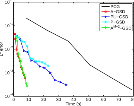
shows the error with respect to computational time for different algorithms. 0 10 20 30 40 50 60 70 80 10−4 10−3 10−2 10−1 100 Time (s) L 2 error PCG A−GSD PU−GSD P−GSD AM+2−GSD
Fig. 14. Comparison between resolution techniques: L2-error versus computational
time (reference discretization)
Arnoldi-type algorithm (A-GSD) leads to significant computational savings compared to PCG but also compared to algorithms P-GSD and PU-GSD, which were proposed in a previous paper [16]. PU-GSD (resp. P-GSD) is a power-type algorithm with deflation and with updating (resp. without updat-ing). We recall that these power-type algorithms are equivalent to a subspace iteration algorithm to build the generalized spectral decomposition. We ob-serve that PU-GSD and P-GSD lead to similar computational times. In fact, the computational time required by the updating step in PU-GSD is balanced by the fact that PU-GSD needs for a lower order of decomposition than P-GSD (the computed modes are more pertinent). We also observe that algorithms
AM+k-GSD and A-GSD lead to similar computational times. Of course, for a
given order of decomposition, AM+k-GSD requires more computational times.
However, this decomposition is more accurate than with A-GSD since the computed modes are more pertinent.
6.6.2 Influence of the dimension of approximation spaces
To go further in the comparison of computational costs, we will analyze the influence of the dimensions P and n of stochastic and deterministic approx-imation spaces. Here, we only compare PCG with the most efficient GSD algorithm, namely the Arnoldi-type algorithm (A-GSD). Four meshes, shown in Figure 15, are used to analyze the influence of n. Meshes 1 to 4 correspond respectively to n = 1150, 1624, 3590 and 6166. To analyze the influence of P , we simply increase the order p of the polynomial chaos expansion of the solution. We will use p = 2, 3 or 4, corresponding to P = 66, 286 or P = 1001 respectively.
Figure 16 (resp. 17) shows the computational times for different p and for the fixed finite element mesh 2 (resp. mesh 4). We can observe than the PCG
(a) mesh 1 : n = 1150
(b) mesh 2 : n = 1624
(c) mesh 3 : n = 3590
(d) mesh 4 : n = 6166
Fig. 15. Different finite element meshes
computational times drastically increase with p while the A-GSD computa-tional times are almost independent of p. More precisely, we notice that when P ≪ n, the computational times required by A-GSD are almost independent of P . This result is clearly observed when we use the fine mesh 4. This is due to the fact that deterministic and stochastic problems are uncoupled. Then, for large n, P has a low influence on computational times, which comes essentially from the resolution of deterministic equations.
Figure 18 (resp. 19) shows the computational times for different n and for a fixed p = 2 (resp. p = 4). We can observe than the PCG computational times drastically increase with n while the A-GSD computational times are almost
0 50 100 150 200 250 300 350 10−4 10−3 10−2 10−1 100 Time (s) L 2 error PCG , p=2 A−GSD , p=2 PCG , p=3 A−GSD , p=3 PCG , p=4 A−GSD , p=4
Fig. 16. Influence of stochastic dimension (variable p) with fixed mesh 2
0 50 100 150 200 250 300 350 400 10−4 10−3 10−2 10−1 100 Time (s) L 2 error PCG , p=2 A−GSD , p=2 PCG , p=3 A−GSD , p=3
Fig. 17. Influence of stochastic dimension (variable p) with fixed mesh 4
independent of n (especially for large P ). This result is clearly observed when we use p = 4 (P = 1001). This is still due to the fact that deterministic and stochastic problems are uncoupled. Then, for large P , n has a low influence on computational times, which comes essentially from the resolution of stochastic equations. 0 20 40 60 80 100 10−4 10−3 10−2 10−1 100 Time (s) L 2 error PCG , mesh 1 A−GSD , mesh 1 PCG , mesh 2 A−GSD , mesh 2 PCG , mesh 3 A−GSD , mesh 3 PCG , mesh 4 A−GSD , mesh 4
Fig. 18. Influence of deterministic dimension (different meshes) with fixed stochastic discretization (p = 2)
0 100 200 300 400 500 600 700 10−4 10−3 10−2 10−1 100 Time (s) L 2 error PCG , mesh 1 A−GSD , mesh 1 PCG , mesh 2 A−GSD , mesh 2 PCG , mesh 3 A−GSD , mesh 3
Fig. 19. Influence of deterministic dimension (different meshes) with fixed stochastic discretization (p = 4)
Finally, Table 1 shows the gains in terms of computational times to reach
a given relative error of 10−2. It also shows the gains in terms of memory
requirements to store the corresponding approximate solution. For the largest P and n, we observe that the computational time with A-GSD is 50 times lower than with PCG and that memory requirements are about 200 times lower. P=66 (p=2) P=286 (p=3) P=1001 (p=4) Tg Mg Tg Mg Tg Mg n=1150 9.3 15.3 15.4 57.3 11.2 133.8 n=1624 8.8 15.9 21.6 60.8 17.2 154.8 n=3590 14.8 16.2 42.6 66.2 33.1 195.7 n=6166 20.2 16.3 51.9 68.3 47.2 215.3 Table 1
Comparison between PCG and A-GSD: computational time gain factor Tg = time(P CG)
time(A−GSD) to reach a relative error of 10−2 and memory gain factor Mg = memory(P CG)
memory(A−GSD) to store the approximate solution
7 Model problem 2: a transient heat diffusion problem
7.1 Formulation of the problem and semi-discretization
We consider a transient heat diffusion equation as a model problem for parabolic stochastic partial differential equations (see Figure 20). The problem reads:
Γ 2 g2 g1 Γ1 Γ 0
Fig. 20. Model problem 2 and associated finite element mesh
find a temperature field u : Ω × (0, T ) × Θ → R such that
c∂tu − ∇ · (κ∇u) = f on Ω × (0, T )
−κ∇u · n = gi on Γi × (0, T ), i = 1, 2
u = 0 on Γ0 × (0, T )
u|t=0 = u0 on Ω (48)
where Ω denotes the spatial domain, (0, T ) the time domain, c and κ the
ma-terial parameters, f the volumic heat source and g1(resp. g2) a normal flux on
a part Γ1 (resp. Γ2) of the boundary. Homogeneous Dirichlet boundary
condi-tions are applied on a part Γ0 of the boundary, which is the complementary
part of Γ1∪ Γ2. For numerical examples, we will take u0 = 0. However, for the
sake of generality, this term is kept in the presentation of the method.
For space discretization, we use four-nodes linear finite elements (see mesh in Figure 20). It classically leads to the following system of stochastic differential
equations in time: find u : (0, T ) × Θ → Rnx such that
M(θ) ˙u(t, θ) + B(θ)u(t, θ) = c(t, θ) (49)
u(0, θ) = u0(θ) (50)
When using a classical time integration scheme, the resulting semi-discretized stochastic problem can formally be written as in equation (1). Let us illus-trate this for the case of a standard backward Euler scheme. We denote by
(0 = t0, t1, . . . , tnt = T ) the time grid. For the sake of simplicity, we
sup-pose that we have a uniform time step δt. Denoting the solution by u(θ) ≡
(u(t1, θ)T, u(t2, θ)T, . . . , u(tnt, θ)
T)T ∈ Rn ⊗ S, with n = n
x × nt, problem
and random vector b are defined by: A= M+ Bδt 0 . . . 0 −M M+ Bδt . .. ... ... . .. . .. 0 0 . . . −M M + Bδt (51) b= c(t1)δt + Mu0 c(t2)δt ... c(tnt)δt (52)
The present model problem is then equivalent to our generic problem (1), whose weak formulation writes (5). For the reference problem, we consider
nx = 1179 and nt = 30.
The generalized spectral decomposition technique can then be directly applied to problem (5). Here, the GSD decomposition (15) reads
u(t, θ) ≈ W(t)Λ(θ) ⇔ u(θ) ≈ WΛ(θ)
where W ≡ (W(t1)T, . . . , W(tnt)
T)T ∈ Rn×M. With the proposed algorithms,
the construction of this decomposition requires the resolution of reduced deter-ministic problems (13) and reduced stochastic problems (11). Of course, this writing is just formal. In practice, those problems are interpreted with re-spect to the initial evolution problem. This interpretation and computational aspects are detailed in appendix C. In particular, it is shown that GSD takes into account initial conditions in a week sense.
7.2 Stochastic modeling and approximation
Material parameters are considered as simple random variables, independent
of space and time. We take c(θ) = ξ1(θ) + ξ2(θ) and κ = ξ3(θ) + ξ4(θ), where
ξ1, . . . , ξ4 ∈ U (0.7, 1.3) 5 are four independent identically distributed uniform
random variables. The volumic heat source is considered as a simple
Gaus-sian random variable, independent of time and space: f = ξ5(θ) ∈ N (1, 0.2).
Normal fluxes are taken as: g1(t, θ) = ξ6(θ)Tt and g2(t, θ) = ξ7(θ)Tt, where
ξ6, ξ7 ∈ N (1, 0.2). The probabilistic content is then represented by m = 7