HAL Id: hal-00412263
https://hal.archives-ouvertes.fr/hal-00412263
Submitted on 15 Apr 2020
HAL is a multi-disciplinary open access
archive for the deposit and dissemination of
sci-entific research documents, whether they are
pub-lished or not. The documents may come from
teaching and research institutions in France or
abroad, or from public or private research centers.
L’archive ouverte pluridisciplinaire HAL, est
destinée au dépôt et à la diffusion de documents
scientifiques de niveau recherche, publiés ou non,
émanant des établissements d’enseignement et de
recherche français ou étrangers, des laboratoires
publics ou privés.
Causal graphical models with latent variables : learning
and inference
Philippe Leray, Stijn Meganck, Sam Maes, Bernard Manderick
To cite this version:
Philippe Leray, Stijn Meganck, Sam Maes, Bernard Manderick. Causal graphical models with latent
variables : learning and inference. Holmes, D. E. and Jain, L. Innovations in Bayesian Networks:
The-ory and Applications, Springer, pp.219-249, 2008, Studies in Computational Intelligence, vol.156/2008,
�10.1007/978-3-540-85066-3_9�. �hal-00412263�
Causal Graphical Models with Latent
Variables: Learning and Inference
Philippe Leray1, Stijn Meganck2, Sam Maes3, and Bernard Manderick2
1 LINA Computer Science Lab UMR6241, Knowledge and Decision Team, Universit´e de Nantes, France philippe.leray@univ-nantes.fr 2 Computational Modeling Lab, Vrije Universiteit Brussel, Belgium
3 LITIS Computer Science, Information Processing and Systems Lab EA4108, INSA Rouen, France
1 Introduction
This chapter discusses causal graphical models for discrete variables that can handle latent variables without explicitly modeling them quantitatively. In the uncertainty in artificial intelligence area there exist several paradigms for such problem domains. Two of them are semi-Markovian causal models and maximal ancestral graphs. Applying these techniques to a problem domain consists of several steps, typically: structure learning from observational and experimental data, parameter learning, probabilistic inference, and, quantita-tive causal inference.
We will start this chapter by introducing causal graphical models without latent variables and then move on to models with latent variables.
We will discuss the problem that each of the existing approaches for causal modeling with latent variables only focuses on one or a few of all the steps involved in a generic knowledge discovery approach. The goal of this chapter is to investigate the integral process from observational and experimental data unto different types of efficient inference.
Semi-Markovian causal models (SMCMs) are an approach developed by (Pearl, 2000; Tian and Pearl, 2002a). They are specifically suited for perform-ing quantitative causal inference in the presence of latent variables. However, at this time no efficient parametrisation of such models is provided and there are no techniques for performing efficient probabilistic inference. Furthermore there are no techniques to learn these models from data issued from observa-tions, experiments or both.
Maximal ancestral graphs (MAGs) are an approach developed by (Richard-son and Spirtes, 2002). They are specifically suited for structure learning in the presence of latent variables from observational data. However, the tech-niques only learn up to Markov equivalence and provide no clues on which additional experiments to perform in order to obtain the fully oriented causal
graph. See Eberhardt et al. (2005); Meganck et al. (2006) for that type of results for Bayesian networks without latent variables. Furthermore, as of yet no parametrisation for discrete variables is provided for MAGs and no tech-niques for probabilistic inference have been developed. There is some work on algorithms for causal inference, but it is restricted to causal inference quanti-ties that are the same for an entire Markov equivalence class of MAGs (Spirtes et al., 2000; Zhang, 2006).
We have chosen to use SMCMs as a final representation in our work, because they are the only formalism that allows to perform causal inference while fully taking into account the influence of latent variables. However, we will combine existing techniques to learn MAGs with newly developed methods to provide an integral approach that uses both observational data and experiments in order to learn fully oriented semi-Markovian causal models.
Furthermore, we have developed an alternative representation for the prob-ability distribution represented by a SMCM, together with a parametrisation for this representation, where the parameters can be learned from data with classical techniques. Finally, we discuss how probabilistic and quantitative causal inference can be performed in these models with the help of the alter-native representation and its associated parametrisation4.
The next section introduces the simplest causal models and their impor-tance. Then we discuss causal models with latent variables. In section 4, we discuss structure learning for those models and in the next section we intro-duce techniques for learning a SMCM with the help of experiments. Then we propose a new representation for SMCMs that can easily be parametrised. We also show how both probabilistic and causal inference can be performed with the help of this new representation.
2 Importance of Causal Models
We start this section by introducing basic notations necessary for the under-standing of the rest of this chapter. Then we will discuss classical probabilistic Bayesian networks followed by causal Bayesian networks. Finally we handle the difference between probabilistic and causal inference, or observation vs. manipulation.
2.1 Notations
In this work, uppercase letters are used to represent variables or sets of vari-ables, i.e. V = {V1, . . . , Vn}, while corresponding lowercase letters are used
4 By the term parametrisation we understand the definition of a complete set of pa-rameters that describes the joint probability distribution which can be efficiently used in computer implementations of probabilistic inference, causal inference and learning algorithms.
to represent their instantiations, i.e. v1, v2 and v is an instantiation of all Vi.
P(Vi) is used to denote the probability distribution over all possible values of
variable Vi, while P (Vi = vi) is used to denote the probability of the
instan-tiation of variable Vi to value vi. Usually, P (vi) is used as an abbreviation of
P(Vi= vi).
The operators P a(Vi), Anc(Vi), N e(Vi) denote the observable parents,
an-cestors and neighbors respectively of variable Viin a graph and P a(vi)
repre-sents the values of the parents of Vi. If Vi ↔ Vj appears in a graph then we
say that they are spouses, i.e. Vi∈ Sp(Vj) and vice versa.
When two variables Vi, Vj are independent we denote it by (Vi⊥⊥Vj), when
they are dependent by (Vi 2Vj).
2.2 Probabilistic Bayesian Networks
Here we briefly discuss classical probabilistic Bayesian networks.
See Figure 1 for a famous example adopted from Pearl (1988) representing an alarm system. The alarm can be triggered either by a burglary, by an earthquake, or by both. The alarm going of might cause John and/or Mary to call the house owner at his office.
Mary Calls John Calls
Alarm Burglary Earthquake P(M=T) 0.01 M T F P(J=T|M) 0.17 0.05 M J P(A=T|M,J) T T T F F T F F 0.76 0.01 0.02 0.00008 P(B=T|A) A T F 0.37 0.00006 A B P(E=T|A,B) T T T F F T F F 0.002 0.37 0.002 0.001
Fig. 1.Example of a Bayesian network representing an alarm system.
In Pearl (1988); Russell and Norvig (1995) probabilistic Bayesian networks are defined as follows:
Definition 1.A Bayesian network is a triple hV, G, P (vi|P a(vi))i, with:
• a directed acyclic graph (DAG) G, where each node represents a variable from V
• parameters: conditional probability distributions (CPD) P (vi|P a(vi)) of
each variable Vi from V conditional on its parents in the graph G.
The CPDs of a BN represent a factorization of the joint probability distri-bution as a product of conditional probability distridistri-butions of each variable given its parents in the graph:
P(v) = Y
Vi∈V
P(vi|P a(vi)) (1)
Inference
A BN also allows to efficiently answer probabilistic queries such as P(burglary = true|Johncalls = true, M arycalls = f alse),
in the alarm example of Figure 1. It is the probability that there was a bur-glary, given that we know John called and Mary did not.
Methods have been developed for efficient exact probabilistic inference when the networks are sparse (Pearl, 1988). For networks that are more com-plex this is not tractable, and approximate inference algorithms have been formulated (Jordan, 1998), such as variational methods (Jordan et al., 1999) and Monte Carlo methods (Mackay, 1999).
Structure Learning
There are two main approaches for learning the structure of a BN from data: score-based learning (Heckerman, 1995) and constraint-based learning (Spirtes et al., 2000; Pearl, 2000).
For score-based learning, the goal is to find the graph that best matches the data by introducing a scoring function that evaluates each network with respect to the data, and then to search for the best network according to this score.
Constraint-based methods are based on matching the conditional indepen-dence relations observed between variables in the data with those entailed by a graph.
However, in general a particular set of data can be represented by more than one BN. Therefore the above techniques have in common that they can only learn upto the Markov equivalence class. Such a class contains all the DAGs that correctly represent the data and for performing probabilistic inference any DAG of the class can be chosen.
2.3 Causal Bayesian Networks
Now we will introduce a category of Bayesian networks where the edges have a causal meaning.
We have previously seen that in general there is more than one probabilistic BN that can be used to represent the same JPD. More specifically, all the members of a given Markov equivalence class can be used to represent the same JPD.
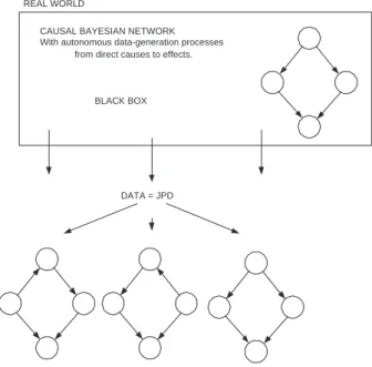
Opposed to that, in the case of a causal Bayesian network (CBN) we assume that in reality there is a single underlying causal Bayesian network that generates the JPD. In Figure 2 we see a conceptual sketch: the box represents the real world where a causal Bayesian network generates the data in the form of a joint probability distribution. Below we see the BNs that represent all the independence relations present in the JPD. Only one of them is the causal Bayesian network, in this case the rightmost.
CAUSAL BAYESIAN NETWORK With autonomous data-generation processes
from direct causes to effects.
BLACK BOX REAL WORLD
DATA = JPD
Fig. 2.Conceptual sketch of how a CBN generates a JPD, that in its turn can be represented by several probabilistic BNs of which one is a CBN.
The definition of causal Bayesian networks is as follows:
Definition 2.A causal Bayesian network is a triple hV, G, P (vi|P a(vi))i,
with:
• a directed acyclic graph (DAG) G, where each node represents a variable from V
• parameters: conditional probability distributions (CPD) P (vi|P a(vi)) of
each variable Vi from V conditional on its parents in the graph G.
• Furthermore, the directed edges in G represent an autonomous causal re-lation between the corresponding variables.
We see that it is exactly the same as Definition 1 for probabilistic Bayesian networks, with the extra addition of the last item.
This is different from a classical BN, where the arrows only represent a probabilistic dependency, and not necessarily a causal one.
Our operational definition of causality is as follows: a relation from variable Cto variable E is causal in a certain context, when a manipulation in the form of a randomised controlled experiment on variable C, induces a change in the probability distribution of variable E, in that specific context (Neapolitan, 2003).
This means that in a CBN, each CPD P (vi|P a(vi)) represents a stochastic
assignment process by which the values of Vi are chosen in response to the
values of P a(Vi) in the underlying domain. This is an approximation of how
events are physically related with their effects in the domain that is being modeled. For such an assignment process to be autonomous means that it must stay invariant under variations in the processes governing other variables Pearl (2000). cloudy rain sprinkler wet lawn cloudy rain wet lawn sprinkler (a) (b)
Fig. 3.(a) A BN where not all the edges have a causal meaning. (b) A CBN that can represent the same JPD as (a).
In the BN of Figure 3(a), these assumptions clearly do not hold for all edges and nodes, since in the underlying physical domain, whether or not it is cloudy is not caused by the state of the variable sprinkler, i.e. whether or not the sprinkler is on.
Moreover, one could want to manipulate the system, for example by chang-ing the way in which the state of the sprinkler is determined by its causes. More specifically, by changing how the sprinkler reacts to the cloudiness. In order to incorporate the effect of such a manipulation of the system into the
model, some of the CPDs have to be changed. However, in a non-causal BN, it is not immediately clear which CPDs have to be changed and exactly how this must be done.
In contrast, in Figure 3(b), we see a causal BN that can represent the same JPD as the BN in (a). Here the extra assumptions do hold. For example, if in the system the state of the sprinkler is caused by the cloudiness, and thus the CPD P (sprinkler|cloudy) represents an assignment process that is an approximation of how the sprinkler is physically related to the cloudiness. Moreover, if the sensitivity of the sprinkler is changed, this will only imply a change in the CPD P (sprinkler|cloudy), but not in the processes governing other variables such as P (rain|cloudy).
Note that CBNs are a subclass of BNs and therefore they allow proba-bilistic inference. In the next section we will discuss what additional type of inference can be performed with them, but first we treat how CBNs can be learned.
Structure Learning
As CBNs are a subset of all BNs, the same techniques as for learning the structure of BNs can be used to learn upto the Markov equivalence class. As mentioned before, for BNs any member of the equivalence can be used.
For CBNs this is not the case, as we look for the orientation of the unique network that can both represent the JPD and the underlying causal influences between the variables. In general, in order to obtain the causal orientation of all the edges, experiments have to be performed, where some variables in the domain are experimentally manipulated and the potential effects on other variables are observed.
Eberhardt et al. (2005) discuss theoretical bounds on the amount of exper-iments that have to be performed to obtain the full oriented CBN. Meganck et al. (2006) have proposed a solution to learning CBNs from experiments and observations, where the total cost of the experiments is minimised by using elements from decision theory.
Other related approaches include Cooper and Yoo (1999) who derived a Bayesian method for learning from an arbitrary mixture of observational and experimental data.
Tong and Koller (2001) provide an algorithm that actively chooses the experiments to perform based on the model learned so far. In this setting they assume there are a number of query variables Q that can be experimented on and then measure the influence on all other variables V \Q. In order to choose the optimal experiment they introduce a loss-function, based on the uncertainty of the direction of an edge, to help indicate which experiment gives the most information. Using the results of their experiments they update the distribution over the possible networks and network parameters. Murphy (2001) introduces a slightly different algorithm of the same approach.
2.4 Causal Inference
Here we will briefly introduce causal inference, we start by pointing out the difference with probabilistic inference, and then move on to discuss an impor-tant theorem related to causal inference.
Observation vs. Manipulation
An important issue in reasoning under uncertainty is to distinguish between different types of conditioning, each of which modify a given probability dis-tribution in response to information obtained.
Definition 3.Conditioning by observation refers to the way in which a probability distribution of Y should be modified when a modeler passively observes the information X = x.
This is represented by conditional probabilities that are defined as follows: P(Y = y|X = x) = P (y|x) = P(Y = y, X = x)
P(X = x) . (2) This type of conditioning is referred to as probabilistic inference. It is used when the modeler wants to predict the behavior of some variables that have not been observed, based on the state of some other variables. E.g. will the patients’ infection cause him to have a fever ?
This can be very useful in a lot of situations, but in some cases the modeler does not merely want to predict the future behavior of some variables, but has to decide which action to perform, i.e. which variable to manipulate in which way. For example, will administering a dose of 10mg of antibiotics cure the patients’ infection ?
In that case probabilistic inference is not the right technique to use, be-cause in general it will return the level of association between the variables instead of the causal influence. In the antibiotics example: if observing the administration of a dose of 10mg of antibiotics returns a high probability of curing the infection, this can be due to (a mix of) several reasons:
• the causal influence of antibiotics on curing the infection, • the causal influence of curing the infection on antibiotics,
• the causal influence of another variable on both antibiotics and curing the infection, or,
• the causal influence of both antibiotics and curing the infection on another variable that we inadvertently condition on (i.e. selection bias).
Without extra information we cannot make the difference between these rea-sons. On the other hand if we want to know whether administering a dose of 10mg of antibiotics will cure the patients’ infection, we will need to isolate the causal influence of antibiotics on curing the infection and this process is denoted by causal inference.
Definition 4.Causal inference is the process of calculating the effect of manipulating some variables X on the probability distribution of some other variables Y .
Definition 5.Conditioning by interventionor manipulation5 refers to
the way the distribution Y should be modified if we intervene externally and force the value of X to be equal to x.
To make the distinction clear, Pearl has introduced the do-operator (Pearl, 2000)6:
P(Y = y|do(X = x)) (3) The manipulations we are treating here are surgical in the sense that they only directly change the variable of interest (X in the case of X = do(x)).
To reiterate, it is important to realize that conditioning by observation is typically not the way the distribution of Y should be modified if we intervene externally and force the value of X to be equal to x, as can be seen next:
P(Y = y|do(X = x)) 6= P (Y = y|X = x) (4) and the quantity on the left-hand side cannot be calculated from the joint probability distribution P (v) alone, without additional assumptions imposed on the graph, i.e. that a directed edge represents an autonomous causal rela-tion as in CBNs.
Consider the simple CBNs of Figure 4 in the left graph P(y|do(x)) = P (y|x)
as X is the only immediate cause of Y , but
P(x|do(y)) = P (x) 6= P (x|y)
as there is no direct or indirect causal relation going from Y to X. The equal-ities above are reversed in the graph to the right, i.e. there it holds that P(y|do(x)) = P (y) 6= P (y|x) and P (x|do(y)) = P (x|y).
X
Y
X
Y
Fig. 4.Two simple causal Bayesian networks.
Next we introduce a theorem that specifies how a manipulation modifies the JPD associated with a CBN.
5 Throughout this chapter the terms intervention and manipulation are used in-terchangeably.
6 In the literature other notations such as P (Y = y||X = x), P
X=x(Y = y), or P(Y = y|X = ˆx) are abundant.
Manipulation Theorem
Performing a manipulation in a domain that is modeled by a CBN, does modify that domain and the JPD that is used to model it. Before introducing a theorem that specifies how a CBN and the JPD that is associated with it must be changed to incorporate the change induced by a manipulation, we will offer an intuitive example.
Example 1. Imagine we want to disable the alarm in the system represented by the CBN of Figure 5(a) by performing the manipulation do(alarm=off ).
This CBN represents an alarm system against burglars, it can be triggered by a burglary, an earthquake or both. Furthermore, the alarm going off might cause the neighbors to call the owner at his work.
alarm burglary earthquake John calls Mary calls do(alarm=off) burglary earthquake John calls Mary calls (a) (b)
Fig. 5. (a) A CBN of an alarm system. (b) The CBN of the alarm system of (a) after disabling the alarm via an external manipulation: do(alarm=off ).
Such a manipulation changes the way in which the value of alarm is being produced in the real world. Originally, the value of alarm was being decided by its immediate causes in the model of Figure 5(a): burglary and earthquake. After manipulating the alarm by disabling it, burglary and earthquake are no longer the causes of the alarm, but have been replaced by the manipulation. In Figure 5(b) the graph of the post-manipulation CBN is shown. There we can see that the links between the original causes of alarm have been severed and that the value of alarm has been instantiated to off.
To obtain the post-manipulation distribution after fixing a set of variables M ⊆ V to fixed values M = m, the factors with the variables in M conditional on their parents in the graph (i.e. their causes in the pre-intervention distribu-tion), have to be removed from the JPD. Formally these are : P (mi|P a(mi))
for all variables Mi ∈ M . This is because after the intervention, it is this
of the variables in M . Furthermore the remaining occurrences of M in the JPD have to be instantiated to M = m.
A manipulation of this type only has a local influence in the sense that only the incoming links of a manipulated variable have to be removed from the model, no factors representing other links have to be modified, except for instantiating the occurrences of the manipulated variables M to m. This is a consequence of the assumption of CBNs that the factors of the JPD represent assignment processes that must stay invariant under variations in the processes governing other variables. Formally, we get from (Spirtes et al., 2000):
Theorem 1.Given a CBN with variables V = V1, . . . , Vn and we perform the
manipulation M = m for a subset of variables M ⊆ V , the post-manipulation distribution becomes: P(v|do(m)) = Y Vi∈V \M P(vi|P a(vi)) M=m (5)
Where |M=m stands for instantiating all the occurrences of the variables M to values m in the equation that precedes it.
3 Causal Models with Latent Variables
In all the above we made the assumption of causal sufficiency, i.e. that for every variable of the domain that is a common cause, observational data can be obtained in order to learn the structure of the graph and the CPDs. Often this assumption is not realistic, as it is not uncommon that a subset of all the variables in the domain is never observed. We refer to such a variable as a latent variable.
We start this section by briefly discussing different approaches to modeling latent variables. After that we introduce two specific models for modeling la-tent variables and the causal influences between the observed variables. These will be the two main formalisms used in the rest of this chapter so we will discuss their semantics and specifically their differences in a lot of detail. 3.1 Modeling Latent Variables
Consider the model in Figure 6(a), it is a problem with observable variables V1, . . . , V6and latent variables L1, L2and it is represented by a directed acyclic
graph (DAG). As this DAG represents the actual problem henceforth we will refer to it as the underlying DAG.
One way to represent such a problem is by using this DAG representation and modeling the latent variables explicitly. Quantities for the observable
V3 V1 V2 V5 V4 V6 L 1 L2 V3 V1 V2 V5 V4 V6 (a) (b) V3 V1 V2 V5 V4 V6 (c)
Fig. 6.(a) A problem domain represented by a causal DAG model with observable and latent variables. (b) A semi-Markovian causal model representation of (a). (c) A maximal ancestral graph representation of (a).
variables can then be obtained from the data in the usual way. Quantities involving latent variables however will have to be estimated. This involves estimating the cardinality of the latent variables and this whole process can be difficult and lengthy. One of the techniques to learn models in such a way is the structural EM algorithm (Friedman, 1997).
Another method to take into account latent variables in a model is by representing them implicitly. With that approach, no values have to be es-timated for the latent variables, instead their influence is absorbed in the distributions of the observable variables. In this methodology, we only keep track of the position of the latent variable in the graph if it would be modeled, without estimating values for it. Both the modeling techniques that we will use in this chapter belong to that approach, they will be described in the next two sections.
3.2 Semi-Markovian Causal Models
The central graphical modeling representation that we use are the semi-Markovian causal models. They were first used by Pearl (2000), and Tian and Pearl (2002a) have developed causal inference algorithms for them. Definitions
Definition 6.A semi-Markovian causal model (SMCM) is an acyclic causal graph G with both directed and bi-directed edges. The nodes in the graph represent observable variables V = {V1, . . . , Vn} and the bi-directed edges
im-plicitly represent latent variables L = {L1, . . . , Ln′}.
See Figure 6(b) for an example SMCM representing the underlying DAG in (a).
The fact that a bi-directed edge represents a latent variable, implies that the only latent variables that can be modeled by a SMCM can not have any parents (i.e. is a root node) and has exactly two children that are both observed. This seems very restrictive, however it has been shown that models with arbitrary latent variables can be converted into SMCMs, while preserving the same independence relations between the observable variables (Tian and Pearl, 2002b).
Semantics
In a SMCM, each directed edge represents an immediate autonomous causal relation between the corresponding variables, just as was the case for causal Bayesian networks.
In a SMCM, a bi-directed edge between two variables represents a latent variable that is a common cause of these two variables.
The semantics of both directed and bi-directed edges imply that SMCMs are not maximal, meaning that not all dependencies between variables are represented by an edge between the corresponding variables. This is because in a SMCM an edge either represents an immediate causal relation or a latent common cause, and therefore dependencies due to a so called inducing path, will not be represented by an edge.
Definition 7.An inducing path is a path in a graph such that each observ-able non-endpoint node is a collider, and an ancestor of at least one of the endpoints.
Inducing paths have the property that their endpoints can not be separated by conditioning on any subset of the observable variables. For instance, in Figure 6(a), the path V1→ V2← L1→ V6is inducing.
Parametrisation
SMCMs cannot be parametrised in the same way as classical Bayesian net-works (i.e. by the set of CPTs P (Vi|P a(Vi))), since variables that are
con-nected via a bi-directed edge have a latent variable as a parent.
For example in Figure 6(b), choosing P (V5|V4) as a parameter to be
associ-ated with variable V5would only lead to erroneous results, as the dependence
with variable V6via the latent variable L2 in the underlying DAG is ignored.
As mentioned before, using P (V5|V4, L2) as a parametrisation and estimating
the cardinality and the values for latent variable L2would be a possible
solu-tion. However we choose not to do this as we want to leave the latent variables implicit for reasons of efficiency.
In (Tian and Pearl, 2002a), a factorisation of the joint probability distri-bution over the observable variables of an SMCM was introduced. Later in this chapter we will derive a representation for the probability distribution represented by a SMCM based on that result.
Learning
In the literature no algorithm for learning the structure of an SMCM exists, in this chapter we introduce techniques to perform that task, given some simplifying assumptions, and with the help of experiments.
Probabilistic Inference
Since as of yet no efficient parametrisation for SMCMs is provided in the literature, no algorithm for performing probabilistic inference exists. We will show how existing probabilistic inference algorithms for Bayesian networks can be used together with our parametrisation to perform that task.
Causal Inference
SMCMs are specifically suited for another type of inference, i.e. causal in-ference. An example causal inference query in the SMCM of Figure 6(a) is P(V6= v6|do(V2= v2)).
As seen before, causal inference queries are calculated via the Manipu-lation Theorem, which specifies how to change a joint probability distribu-tion (JPD) over observable variables in order to obtain the post-manipuladistribu-tion JPD. Informally, it says that when a variable X is manipulated to a fixed value x, the parents of variables X have to be removed by dividing the JPD by P (X|P a(X)), and by instantiating the remaining occurrences of X to the value x.
When all the parents of a manipulated variable are observable, this can always be done. However, in a SMCM some of the parents of a manipulated variable can be latent and then the Manipulation Theorem cannot be directly used to calculate causal inference queries. Some of these causal quantities can be calculated in other ways but some cannot be calculated at all, because the SMCM does not contain enough information.
When a causal query can be unambiguously calculated from a SMCM, we say that it is identifiable. More formally:
Definition 8.The causal effect of variable X on a variable Y is identifiable from a SMCM with graph G if PM1(y|do(x)) = PM2(y|do(x)) for every pair of
SMCMs M1and M2 with PM1(v) = PM2(v) > 0 and GM1 = GM2, where PMi
and GMi respectively denote the probability distribution and graph associated
with the SMCM Mi.
In Pearl (2000), Pearl describes the do-calculus, a set of inference rules and an algorithm that can be used to perform causal inference. More specifically, the goal of do-calculus is to transform a mathematical expression including manipulated variables related to a SMCM into an equivalent expression in-volving only standard probabilities of observed quantities. Recent work has
shown that do-calculus is complete (Huang and Valtorta, 2006; Shpitser and Pearl, 2006).
Tian and Pearl have introduced theoretical causal inference algorithms to perform causal inference in SMCMs (Pearl, 2000; Tian and Pearl, 2002a). However, these algorithms assume the availability of a subset of all the con-ditional distributions that can be obtained from the JPD over the observable variables. We will show that with our representation these conditional distri-butions can be obtained in an efficient way in order to apply this algorithm. 3.3 Maximal Ancestral Graphs
Maximal ancestral graphs are another approach to modeling with latent vari-ables developed by Richardson and Spirtes (2002). The main research focus in that area lies on learning the structure of these models and on representing ex-actly all the independences between the observable variables of the underlying DAG.
Definitions
Ancestral graphs (AGs) are graphs that are complete under marginalisation and conditioning. We will only discuss AGs without conditioning as is com-monly done in recent work (Zhang and Spirtes, 2005b; Tian, 2005; Ali et al., 2005).
Definition 9.An ancestral graph without conditioning is a graph with no directed cycle containing directed → and bi-directed ↔ edges, such that there is no bi-directed edge between two variables that are connected by a directed path.
Definition 10.An ancestral graph is said to be a maximal ancestral graph if, for every pair of non-adjacent nodes Vi, Vj there exists a set Z such that
Vi and Vj are d-separated given Z.
A non-maximal AG can be transformed into a unique MAG by adding some bi-directed edges (indicating confounding) to the model. See Figure 6(c) for an example MAG representing the same model as the underlying DAG in (a). Semantics
In this setting a directed edge represents an ancestral relation in the under-lying DAG with latent variables. I.e. an edge from variable A to B represents that in the underlying causal DAG with latent variables, there is a directed path between A and B.
Bi-directed edges represent a latent common cause between the variables. However, if there is a latent common cause between two variables A and B,
and there is also a directed path between A and B in the underlying DAG, then in the MAG the ancestral relation takes precedence and a directed edge will be found between the variables. V2→ V6 in Figure 6(c) is an example of
such an edge.
Furthermore, as MAGs are maximal, there will also be edges between variables that have no immediate connection in the underlying DAG, but that are connected via an inducing path. The edge V1→ V6 in Figure 6(c) is
an example of such an edge.
These semantics of edges make some causal inferences in MAGs impossible. As we have discussed before the Manipulation Theorem states that in order to calculate the causal effect of a variable A on another variable B, the immediate parents (i.e. the old causes) of A have to be removed from the model. However, as opposed to SMCMs, in MAGs an edge does not necessarily represent an immediate causal relationship, but rather an ancestral relationship and hence in general the modeler does not know which are the real immediate causes of a manipulated variable.
An additional problem for finding the original causes of a variable in MAGs is that when there is an ancestral relation and a latent common cause between variables, that the ancestral relation takes precedence and that the confound-ing is absorbed in the ancestral relation.
Learning
There is a lot of recent research on learning the structure of MAGs from ob-servational data. The Fast Causal Inference (FCI) algorithm (Spirtes et al., 1999), is a constraint based learning algorithm. Together with the rules dis-cussed in Zhang and Spirtes (2005a), the result is a representation of the Markov equivalence class of MAGs. This representative is referred to as a complete partial ancestral graph (CPAG) and in Zhang and Spirtes (2005a) it is defined as follows:
Definition 11.Let [G] be the Markov equivalence class for an arbitrary MAG G. The complete partial ancestral graph (CPAG) for [G], PG, is a graph
with possibly the following edges →, ↔, o−o, o→, such that
1. PG has the same adjacencies as G (and hence any member of [G]) does;
2. A mark of arrowhead (>) is in PG if and only if it is invariant in [G];
and
3. A mark of tail (−) is in PG if and only if it is invariant in [G].
4. A mark of (o) is in PG if not all members in [G] have the same mark.
In the next section we will discuss learning the structure in somewhat more detail.
Parametrisation and Inference
At this time no parametrisation for MAGs with discrete variables exists that represents all the properties of a joint probability distribution, (Richardson and Spirtes, 2002), neither are there algorithms fo probabilistic inference.
As mentioned above, due to the semantics of the edges in MAGs, not all causal inferences can be performed. However, there is an algorithm due to Spirtes et al. (2000) and refined by Zhang (2006), for performing causal inference in some restricted cases. More specifically, they consider a causal effect to be identifiable if it can be calculated from all the MAGs in the Markov equivalence class that is represented by the CPAG and that quantity is equal for all those MAGs. This severely restricts the causal inferences that can be made, especially if more than conditional independence relations are taken into account during the learning process, as is the case when experiments can be performed. In the context of this causal inference algorithm, Spirtes et al. (2000) also discuss how to derive a DAG that is a minimal I -map of the probability distribution represented by a MAG.
In this chapter we introduce a similar procedure, but for a single SMCM instead of for an entire equivalence class of MAGs. In that way a larger class of causal inferences can be calculated, as the quantities do not have to be equal in all the models of the equivalence class.
4 Structure Learning with Latent Variables
Just as learning a graphical model in general, learning a model with latent variables consists of two parts: structure learning and parameter learning. Both can be done using data, expert knowledge and/or experiments. In this section we discuss structure learning and we differentiate between learning from observational and experimental data.
4.1 From Observational Data
In order to learn graphical models with latent variables from observational data a constraint based learning algorithm has been developed by Spirtes et al. (1999). It is called the Fast Causal Inference (FCI) algorithm and it uses conditional independence relations found between observable variables to learn a structure.
Recently this result has been extended with the complete tail augmen-tation rules introduced in Zhang and Spirtes (2005a). The results of this algorithm is a CPAG, representing the Markov equivalence class of MAGs consistent with the data.
Recent work in the area consists of characterising the equivalence class of CPAGs and finding single-edge operators to create equivalent MAGs (Ali and Richardson, 2002; Zhang and Spirtes, 2005a,b). One of the goals of these
advances is to create methods that search in the space of Markov equivalent models (CPAGs) instead of the space of all models (MAGs), mimicking results in the case without latent variables (Chickering, 2002).
As mentioned before for MAGs, in a CPAG the directed edges have to be interpreted as representing ancestral relations instead of immediate causal relations. More precisely, this means that there is a directed edge from Vi to
Vj if Vi is an ancestor of Vj in the underlying DAG and there is no subset of
observable variables D such that (Vi⊥⊥Vj|D). This does not necessarily mean
that Vi has an immediate causal influence on Vj, it may also be a result of
an inducing path between Vi and Vj. For instance in Figure 6(c), the link
between V1and V6is present due to the inducing path V1, V2, L1, V6shown in
Figure 6(a).
Inducing paths may also introduce ↔, →, o→ or o−o between two variables, although there is no immediate influence in the form of an immediate causal influence or latent common cause between the two variables. An example of such a link is V3o−oV4in Figure 7.
A consequence of these properties of MAGs and CPAGs is that they are not very suited for general causal inference, since the immediate causal parents of each observable variable are not available as is necessary according to the manipulation theorem. As we want to learn models that can perform causal inference, we will discuss how to transform a CPAG into a SMCM next. 4.2 From Experimental Data
As mentioned above, the result of current state-of-the-art techniques that learn models with implicit latent variables from observational data is a CPAG. This is a representative of the Markov equivalence class of MAGs. Any MAG in that class will be able to represent the same JPD over the observable variables, but not all those MAGs will have all edges with a correct causal orientation.
Furthermore as mentioned in the above, in MAGs the directed edges do not necessarily have an immediate causal meaning as in CBNs or SMCMs, instead they have an ancestral meaning. If it is your goal to perform causal inference, you will need to know the immediate parents to be able to reason about all causal queries. However, edges that are completely oriented but that do not have a causal meaning will not occur in the CPAG, there they will always be of the types o→ or o−o, so orienting them in correct causal way way suffices. Finally, MAGs are maximal, thus every missing edge must represent a con-ditional independence. In the case that there is an inducing path between two variables and no edge in the underlying DAG, the result of the current learn-ing algorithms will be to add an edge between the variables. Again, although these type of edges give the only correct representation of the conditional inde-pendence relations in the domain, they do not represent an immediate causal relation (if the inducing edge is directed) or a real latent common cause (if the inducing edge is bi-directed). Because of this they could interfere with
causal inference algorithms, therefore we would like to identify and remove these type of edges.
To recapitulate, the goal of techniques aiming at transforming a CPAG must be twofold:
• finding the correct causal orientation of edges that are not completely specified by the CPAG (o→ or o−o), and,
• removing edges due to inducing paths.
In the next section we discuss how these goals can be obtained by per-forming experiments.
5 From CPAG to SMCM
Our goal is to transform a given CPAG in order to obtain a SMCM that corresponds to the underlying DAG. Remember that in general there are four types of edges in a CPAG: ↔, →, o→, o−o, in which o means either a tail mark − or a directed mark >. As mentioned before, one of the tasks to obtain a valid SMCM is to disambiguate those edges with at least one o as an endpoint. A second task will be to identify and remove the edges that are created due to an inducing path.
In the next section we will introduced some simplfying assumptions we have to use in our work. Then we will discuss exactly which information is obtained from performing an experiment. After that, we will discuss the two possible incomplete edges: o→ and o−o. Finally, we will discuss how we can find edges that are created due to inducing paths and how to remove them to obtain the correct SMCM.
5.1 Assumptions
As is customary in the graphical modeling research area, the SMCMs we take into account in this chapter are subject to some simplifying assumptions:
1. Stability, i.e. the independencies in the underlying CBN with observed and latent variables that generates the data are structural and not due to several influences exactly cancelling each other out (Pearl, 2000).
2. Only a single immediate connection per two variables in the underlying DAG. I.e. we do not take into account problems where two variables that are connected by an immediate causal edge are also confounded by a la-tent variable causing both variables. Constraint based learning techniques such as IC* (Pearl, 2000) and FCI (Spirtes et al., 2000) also do not explic-itly recognise multiple edges between variables. However, Tian and Pearl (2002a) presents an algorithm for performing causal inference where such relations between variables are taken into account.
3. No selection bias. Mimicking recent work, we do not take into account latent variables that are conditioned upon, as can be the consequence of selection effects.
4. Discrete variables. All the variables in our models are discrete.
5. Correctness. The CPAG is correctly learned from data with the FCI al-gorithm and the extended tail augmentation rules, i.e. each result that is found is not due to a sampling error or insufficient sample size.
5.2 Performing Experiments
The experiments discussed here play the role of the manipulations discussed in Section 2.3 that define a causal relation. An experiment on a variable Vi, i.e.
a randomised controlled experiment, removes the influence of other variables in the system on Vi. The experiment forces a distribution on Vi, and thereby
changes the joint distribution of all variables in the system that depend di-rectly or indidi-rectly on Vi but does not change the conditional distribution of
other variables given values of Vi. After the randomisation, the associations
of the remaining variables with Viprovide information about which variables
Vi influences (Neapolitan, 2003). To perform the actual experiment we have
to cut all influence of other variables on Vi. Graphically this corresponds to
removing all incoming arrows into Vi from the underlying DAG.
We then measure the influence of the manipulation on variables of interest by obtaining samples from their post-experimental distributions.
More precisely, to analyse the results of an experiment on a variable Vexp,
we compare for each variable of interest Vj the original observational sample
data Dobswith the post-experimental sample data Dexp. The experiment
con-sists of manipulating the variable Vexp to each of its values vexp a sufficient
amount of times in order to obtain sample data sets that are large enough to analyse in a statistically sound way. The result of an experiment will be a data set of samples for the variables of interest for each value i of variable Vexp= i, we will denote such a data set by Dexp,i.
In order to see whether an experiment on Vexp made an influence on
an-other variable Vj, we compare each post-experimental data set Dexp,i with
the original observational data set Dobs (with a statistical test like χ2). Only
if at least one of the data sets is statistically significantly different, we can conclude that variable Vexpcausally influences variable Vj.
However, this influence does not necessarily have to be immediate between the variables Vexpand Vj, but can be mediated by other variables, such as in
the underlying DAG: Vexp→ Vmed→ Vj.
In order to make the difference between a direct influence and a potentially mediated influence via Vmed, we will no longer compare the complete data
sets Dexp,i and Dobs. Instead, we will divide both data sets in subsets based
on the values of Vmed, or in other words condition on variable Vmed. Then
we compare each of the smaller data sets Dexp,i|vmed and Dobs|vmed with
Ao→ B Type 1(a) Type 1(b) Type 1(c)
Exper. exp(A) 6 B exp(A) B exp(A) B
result 6 ∃p.d. path A 99K B ∃p.d. path A 99K B
(length ≥ 2) (length ≥ 2)
Orient. A ↔ B A→ B Block all p.d. paths by
result conditioning on
block-ing set Z:
exp(A)|Z B: A → B exp(A)|Z 6 B: A ↔ B Table 1.An overview of how to complete edges of type o→.
mediating variable, we block the causal influence that might go through that variable and we obtain the immediate relation between Vexpand Vj.
Note that it might seem that if the mediating variable is a collider, this approach will fail, because conditioning on a collider on a path between two variables creates a dependence between those two variables. However, this approach will still be valid and this is best understood with an example: imagine the underlying DAG is of the form Vexp· · · → Vmed← . . . Vj. In this
case, when we compare each Dexp,iand Dobsconditional on Vmed, we will find
no significant difference between both data sets, and this for all the values of Vmed. This is because the dependence that is created between Vexpand Vjby
conditioning on the collider Vmed is present in both the original underlying
DAG and in the post-experimental DAG, and thus this is also reflected in the data sets Dexp,i and Dobs.
In order not to overload that what follows with unnecessary complicated notation we will denote performing an experiment at variable Vi or a set of
variables W by exp(Vi) or exp(W ) respectively, and if we have to condition
on some other set of variables Z on the data obtained by performing the experiment, we denote it as exp(Vi)|Z and exp(W )|Z.
In general if a variable Vi is experimented on and another variable Vj is
affected by this experiment, i.e. has another distribution after the experiment than before, we say that Vj varies with exp(Vi), denoted by exp(Vi) Vj. If
there is no variation in Vj we note exp(Vi) 6 Vj.
Before going to the actual solutions we have to introduce the notion of potentially directed paths:
Definition 12.A potentially directed path (p.d. path) in a CPAG is a path made only of edges of types o→ and →, with all arrowheads in the same direction. A p.d. path from Vi to Vj is denoted as Vi99K Vj.
5.3 Solving o→
Ao−oB Type 2(a) Type 2(b) Type 2(c)
Exper. exp(A) 6 B exp(A) B exp(A) B
result 6 ∃p.d. path A 99K B ∃p.d. path A 99K B
(length ≥ 2) (length ≥ 2)
Orient. A ←oB A→ B Block all p.d. paths by
result (⇒Type 1) conditioning on
block-ing set Z:
exp(A)|Z B: A → B exp(A)|Z 6 B: A ←oB (⇒Type 1)
Table 2.An overview of how to complete edges of type o−o.
For any edge Vio→ Vj, there is no need to perform an experiment at Vj
because we know that there can be no immediate influence of Vj on Vi, so we
will only perform an experiment on Vi.
If exp(Vi) 6 Vj, then there is no influence of Vi on Vj so we know that
there can be no directed edge between Vi and Vj and thus the only remaining
possibility is Vi↔ Vj (Type 1(a)).
If exp(Vi) Vj, then we know for sure that there is an influence of Vi
on Vj, we now need to discover whether this influence is immediate or via
some intermediate variables. Therefore we make a difference whether there is a potentially directed (p.d.) path between Vi and Vj of length ≥ 2, or not. If
no such path exists, then the influence has to be immediate and the edge is found Vi→ Vj (Type 1(b)).
If at least one p.d. path Vi 99K Vj exists, we need to block the influence
of those paths on Vj while performing the experiment, so we try to find a
blocking set Z for all these paths. If exp(Vi)|Z Vj, then the influence has
to be immediate, because all paths of length ≥ 2 are blocked, so Vi→ Vj. On
the other hand if exp(Vi)|Z 6 Vj, there is no immediate influence and the
edge is Vi↔ Vj (Type 1(c)).
A blocking set Z consists of one variable for each p.d. path. This variable can be chosen arbitrarily as we have explained before that conditioning on a collider does not invalidate our experimental approach.
5.4 Solving o−o
An overview of the different rules for solving o−o is given in Table 2.
For any edge Vio−oVj, we have no information at all, so we might need to
perform experiments on both variables.
If exp(Vi) 6 Vj, then there is no influence of Vi on Vj so we know that
there can be no directed edge between Vi and Vj and thus the edge is of the
following form: Vi ←oVj, which then becomes a problem of Type 1.
If exp(Vi) Vj, then we know for sure that there is an influence of Vion
directed path between Vi and Vj of length ≥ 2, or not. If no such path exists,
then the influence has to be immediate and the edge becomes Vi→ Vj.
If at least one p.d. path Vi 99K Vj exists, we need to block the influence
of those paths on Vj while performing the experiment, so we find a blocking
set Z like with Type 1(c). If exp(Vi)|Z Vj, then the influence has to be
immediate, because all paths of length ≥ 2 are blocked, so Vi → Vj. On the
other hand if exp(Vi)|Z 6 Vj, there is no immediate influence and the edge
is of the following form: Vi←oVj, which again becomes a problem of Type 1.
5.5 Removing Inducing Path Edges
In the previous phase only o-parts of edges of a CPAG have been oriented. The graph that is obtained in this way can contain both directed and bi-directed edges, each of which can be of two types. For the directed edges:
• an immediate causal edge that is also present in the underlying DAG • an edge that is due to an inducing path in the underlying DAG. For the bi-directed edges:
• an edge that represents a latent variable in the underlying DAG • an edge that is due to an inducing path in the underlying DAG.
When representing the same underlying DAG, a SMCM and the graph ob-tained after orienting all unknown endpoints of the CPAG have the same connections except for edges due to inducing paths in the underlying DAG, these edges are only represented in the experimentally oriented graph. Definition 13.We will call an edge between two variables Vi and Vj i-false
if it was created due to an inducing path, i.e. because the two variables are dependent conditional on any subset of observable variables.
For instance in Figure 6(a), the path V1, V2, L1, V6 is an inducing path,
which causes the FCI algorithm to find an i-false edge between V1 and V6,
see Figure 6(c). Another example is given in Figure 7 where the SMCM is given in (a) and the result of FCI in (b). The edge between V3 and V4 in
(b) is a consequence of the inducing path through the observable variables V3, V1, V2, V4.
In order to be able to apply a causal inference algorithm we need to remove all i-false edges from the learned structure. The substructures that can indicate this type of edges can be identified by looking at any two variables that a) are connected by an edge, and, b) have at least one inducing path between them. To check whether the immediate connection needs to be present we have to block all inducing paths by performing one or more experiments on an inducing path blocking set (i-blocking set) Zip and block all other open paths
by conditioning on a blocking set Z. Note that the set of variables Zipare the
V1 V2
V3 V4
V1 V2
V3 V4
(a) (b)
Fig. 7.(a) A SMCM. (b) Result of FCI, with an i-false edge V3o−oV4. Given A MAG with a pair of connected variables Vi, Vj,
and a set of inducing paths Vi, . . . , Vj
Action Block all inducing paths Vi, . . . , Vj by performing exper-iments on i-blocking set Zip.
Block all other open paths between Viand Vjby condition-ing on blockcondition-ing set Z.
When performing all exp(Zip)|Z: if (Vi 2Vj): - confounding is real
- else remove edge between Vi, Vj Table 3.Removing i-false edges.
of variables Z are used when looking for independences in the interventional data. If Vi and Vjare dependent, i.e. (Vi 2Vj), under these circumstances then
the edge is correct and otherwise it can be removed.
In the example of Figure 6(c), we can block the inducing path by perform-ing an experiment on V2, and hence can check that V1 and V6do not covary
with each other in these circumstances, so the edge can be removed.
An i-blocking set consists of a collider on each of the inducing paths con-necting the two variables of interest. Here a blocking set Z is a set of variables that blocks each of the other open paths between the two variables of interest.
Table 3 gives an overview of the actions to resolve i-false edges. 5.6 Example
We will demonstrate a number of steps to discover the completely oriented SMCM (Figure 6(b)) based on the result of the FCI algorithm applied on observational data generated from the underlying DAG in Figure 6(a). The result of the FCI algorithm can be seen in Figure 8(a). We will first resolve problems of Type 1 and 2, and then remove i-false edges. The result of each step is explained in Table 4 and indicated in Figure 8.
After resolving all problems of Type 1 and 2 we end up with the structure shown in Figure 8(f), this representation is no longer consistent with the MAG representation since there are bi-directed edges between two variables on a directed path, i.e. V2, V6. However, this structure is not necessarily a
V3 V1 V2 V5 V4 V6 V3 V1 V2 V5 V4 V6 V3 V1 V2 V5 V4 V6 (b) (c) (d) (e) V3 V1 V2 V5 V4 V6 V3 V1 V2 V5 V4 V6 (f) V3 V1 V2 V5 V4 V6 (a)
Fig. 8. (a) The result of FCI on data of the underlying DAG of Figure 6(a). (b) Result of an experiment at V5. (c) Result after experiment at V4. (d) Result after experiment at V3. (e) Result after experiment at V2 while conditioning on V3. (f) Result of resolving all problems of Type 1 and 2.
Exper. Edge Experiment Edge Type
before result after
exp(V5) V5o−oV4 exp(V5) 6 V4 V5←oV4 Type 2(a) V5o→ V6 exp(V5) 6 V6 V5↔ V6 Type 1(a) exp(V4) V4o−oV2 exp(V4) 6 V2 V4←oV2 Type 2(a) V4o−oV3 exp(V4) 6 V3 V4←oV3 Type 2(a) V4o→ V5 exp(V4) V5 V4→ V5 Type 1(b) V4o→ V6 exp(V4) V6 V4→ V6 Type 1(b) exp(V3) V3o−oV2 exp(V3) 6 V2 V3←oV2 Type 2(a) V3o→ V4 exp(V3) V4 V3→ V4 Type 1(b) exp(V2) V2o−oV1 exp(V2) 6 V1 V2←oV1 Type 2(a) V2o→ V3 exp(V2) V3 V2→ V3 Type 1(b) V2o→ V4 exp(V2)|V3 V4V2→ V4 Type 1(c)
Table 4.Example steps in disambiguating edges by performing experiments.
with inducing path V1, V2, V6, so we need to perform an experiment on V2,
blocking all other paths between V1 and V6 (this is also done by exp(V2) in
this case). Given that the original structure is as in Figure 6(a), performing exp(V2) shows that V1 and V6 are independent, i.e. exp(V2) : (V1⊥⊥V6). Thus
the bi-directed edge between V1 and V6 is removed, giving us the SMCM of
Figure 6(b).
6 Parametrisation of SMCMs
As mentioned before, in his work on causal inference, Tian provides an al-gorithm for performing causal inference given knowledge of the structure of an SMCM and the joint probability distribution (JPD) over the observable variables. However, a parametrisation to efficiently store the JPD over the observables is not provided.
We start this section by discussing the factorisation for SMCMs intro-duced in Tian and Pearl (2002a). From that result we derive an additional representation for SMCMs and a parametrisation of that representation that facilitates probabilistic and causal inference. We will also discuss how these parameters can be learned from data.
6.1 Factorising with Latent Variables
Consider an underlying DAG with observable variables V = {V1, . . . , Vn} and
latent variables L = {L1, . . . , Ln′}. Then the joint probability distribution can
be written as the following mixture of products:
P(v) = X {lk|Lk∈L} Y Vi∈V P(vi|P a(vi), LP a(vi)) Y Lj∈L P(lj), (6)
where LP a(vi) are the latent parents of variable Vi and P a(vi) are the
ob-servable parents of Vi.
Remember that in a SMCM the latent variables are implicitly represented by bi-directed edges, then consider the following definition.
Definition 14.In a SMCM, the set of observable variables can be partitioned into disjoint groups by assigning two variables to the same group iff they are connected by a bi-directed path. We call such a group a c-component (from ”confounded component”) (Tian and Pearl, 2002a).
E.g. in Figure 6(b) variables V2, V5, V6belong to the same c-component. Then
it can be readily seen that c-components and their associated latent variables form respective partitions of the observable and latent variables. Let Q[Si]
denote the contribution of a c-component with observable variables Si ⊂ V
to the mixture of products in equation 6. Then we can rewrite the JPD as follows:
P(v) = Y
i∈{1,...,k}
Given a SMCM G and a topological order O, the PR-representation has these properties: 1. The nodes are V , the observable variables of the SMCM. 2. The directed edges that are present in the SMCM are also
present in the PR-representation.
3. The bi-directed edges in the SMCM are replaced by a number of directed edges in the following way:
Add an edge from node Vi to node Vjiff:
a) Vi∈ (Tj∪ P a(Tj)), where Tjis the c-component of G reduced to variables V(j)that contains Vj,
b) except if there was already an edge between nodes Viand Vj. Table 5.Obtaining the parametrised representation from a SMCM.
Finally, Tian and Pearl (2002a) proved that each Q[S] could be calculated as follows. Let Vo1 < . . . < Von be a topological order over V , and let V
(i)= {Vo1, . . . , Voi}, i = 1, . . . , n and V (0)= ∅. Q[S] = Y Vi∈S P(vi|(Ti∪ P a(Ti))\{Vi}) (8)
where Ti is the c-component of the SMCM G reduced to variables V(i), that
contains Vi. The SMCM G reduced to a set of variables V′ ⊂ V is the graph
obtained by removing all variables V \V′ from the graph and the edges that
are connected to them.
In the rest of this section we will develop a method for deriving a DAG from a SMCM. We will show that the classical factorisation Q P (vi|P a(vi))
associated with this DAG, is the same as the one that is associated with the SMCM as above.
6.2 Parametrised Representation
Here we first introduce an additional representation for SMCMs, then we show how it can be parametrised and finally, we discuss how this new representation could be optimised.
PR-representation
Consider Vo1 < . . . < Von to be a topological order O over the observable
variables V , and let V(i)= {V
o1, . . . , Voi}, i = 1, . . . , n and V
(0) = ∅. Then
Table 5 shows how the parametrised (PR-) representation can be obtained from the original SMCM structure.
What happens is that each variable becomes a child of the variables it would condition on in the calculation of the contribution of its c-component as in Equation (8).
V3 V1 V2 V5 V4 V6 V1,V2,V4,V5,V6 V2,V4 V2,V3,V4 (a) (b)
Fig. 9.(a) The PR-representation applied to the SMCM of Figure 6(b). (b) Junction tree representation of the DAG in (a).
In Figure 9(a), the PR-representation of the SMCM in Figure 6(a) can be seen. The topological order that was used here is V1 < V2 < V3 < V4 <
V5< V6 and the directed edges that have been added are V1→ V5, V2→ V5,
V1→ V6, V2→ V6, and, V5→ V6.
The resulting DAG is an I -map (Pearl, 1988), over the observable variables of the independence model represented by the SMCM. This means that all the independencies that can be derived from the new graph must also be present in the JPD over the observable variables. This property can be more formally stated as the following theorem.
Theorem 2.The PR-representation P R derived from a SMCM S is an I-mapof that SMCM.
Proof. Proving that P R is an I -map of S amounts to proving that all inde-pendences represented in P R (A) imply an independence in S (B), or A ⇒ B. We will prove that assuming both A and ¬B leads to a contradiction.
Assumption ¬B: consider that two observable variables X and Y are de-pendent in the SMCM S conditional on some (possible empty) set of observ-able variobserv-ables Z: X 2SY|Z.
Assumpion A: consider that X and Y are independent in P R conditional on Z: X⊥⊥P RY|Z.
Then based on X 2SY|Z we can discriminate two general cases:
1. ∃ a path C in S connecting variables X and Y that contains no colliders and no elements of Z.
2. ∃ a path C in S connecting variables X and Y that contains at least one collider Zi that is an element of Z. For the collider there are three
possibilities:
a) X . . . Ci→ Zi← Cj. . . Y
b) X . . . Ci↔ Zi← Cj. . . Y
c) X . . . Ci↔ Zi↔ Cj. . . Y
1. Transforming S into P R only adds edges and transforms double-headed edges into single headed edges, hence the path C is still present in S and it still contains no collider. This implies that X⊥⊥P RY|Z is false.
2. a) The path C is still present in S together with the collider in Zi, as
it has single headed incoming edges. This implies that X⊥⊥P RY|Z is
false.
b) The path C is still present in S. However, the double-headed edge is transformed into a single headed edge. Depending on the topological order there are two possibilities:
• Ci→ Zi ← Cj: in this case the collider is still present in P R, this
implies that X 2P RY|Z
• Ci ← Zi ← Cj: in this case the collider is no longer present, but
in P R there is the new edge Ci← Cj and hence X 2P RY|Z
c) The path C is still present in S. However, both double-headed edges are transformed into single headed edges. Depending on the topologi-cal order there are several possibilities. For the sake of brievity we will only treat a single order here, for the others it can easily be checked that the same holds.
If the order is Ci< Zi< Cj, the graph becomes Ci → Zi → Cj, but
there are also edges from Ci and Zi to Cj and its parents P a(Cj).
Thus the collider is no longer present, but the extra edges ensure that X 2P RY|Z.
This implies that X⊥⊥P RY|Z is false and therefore we can conclude that P R
is always an I -map of S under our assumptions. ⊓⊔ Parametrisation
For this DAG we can use the same parametrisation as for classical BNs, i.e. learning P (vi|P a(vi)) for each variable, where P a(vi) denotes the parents in
the new DAG. In this way the JPD over the observable variables factorises as in a classical BN, i.e. P (v) =Q P (vi|P a(vi)). This follows immediately from
the definition of a c-component and from Equation (8). Optimising the Parametrisation
Remark that the number of edges added during the creation of the PR-representation depends on the topological order of the SMCM.
As this order is not unique, giving precedence to variables with a lesser amount of parents, will cause less edges to be added to the DAG. This is because added edges go from parents of c-component members to c-component members that are topological descendants.
By choosing an optimal topological order, we can conserve more condi-tional independence relations of the SMCM and thus make the graph more sparse, leading to a more efficient parametrisation.
Note that the choice of the topological order does not influence the cor-rectness of the representation, Theorem 2 shows that it will always be an I -map.
Learning Parameters
As the PR-representation of SMCMs is a DAG as in the classical Bayesian network formalism, the parameters that have to be learned are P (vi|P a(vi)).
Therefore, techniques such as ML and MAP estimation (Heckerman, 1995) can be applied to perform this task.
6.3 Probabilistic Inference
Two of the most famous existing probabilistic inference algorithms for mod-els without latent variables are the λ − π algorithm (Pearl, 1988) for tree-structured BNs, and the junction tree algorithm (Lauritzen and Spiegelhalter, 1988) for arbitrary BNs.
These techniques cannot immediately be applied to SMCMs for two rea-sons. First of all until now no efficient parametrisation for this type of models was available, and secondly, it is not clear how to handle the bi-directed edges that are present in SMCMs.
We have solved this problem by first transforming the SMCM to its PR-representation which allows us to apply the junction tree (JT) inference al-gorithm. This is a consequence of the fact that, as previously mentioned, the PR-representation is an I -map over the observable variables. And as the JT algorithm only uses independencies in the DAG, applying it to an I -map of the problem gives correct results. See Figure 9(b) for the junction tree obtained from the parametrised representation in Figure 9(a).
Note that any other classical probabilistic inference technique that only uses conditional independencies between variables could also be applied to the PR-representation.
6.4 Causal Inference
In Tian and Pearl (2002a), an algorithm for performing causal inference was developed, however as mentioned before they have not provided an efficient parametrisation.
In Spirtes et al. (2000); Zhang (2006), a procedure is discussed that can identify a limited amount of causal inference queries. More precisely only those whose result is equal for all the members of a Markov equivalence class represented by a CPAG.
In Richardson and Spirtes (2003), causal inference in AGs is shown on an example, but a detailed approach is not provided and the problem of what to do when some of the parents of a variable are latent is not solved.
By definition in the PR-representation, the parents of each variable are exactly those variables that have to be conditioned on in order to obtain the factor of that variable in the calculation of the c-component, see Table 5 and Tian and Pearl (2002a). Thus, if we want to apply Tian’s causal inference algorithm, the PR-representation provides all the necessary quantitative in-formation, while the original structure of the SMCM provides the necessary structural information.
7 Conclusions and Perspectives
In this chapter we have introduced techniques for causal graphical modeling with latent variables. We have discussed all classical steps in a modeling pro-cess such as learning the structure from observational and experimental data, model parametrisation, probabilistic and causal inference.
More precisely we showed that there is a big gap between the models that can be learned from data alone and the models that are used in causal inference theory. We showed that it is important to retrieve the fully oriented structure of a SMCM, and discussed how to obtain this from a given CPAG by performing experiments.
As the experimental learning approach relies on randomized controlled experiments, in general it is not scalable to problems with a large number of variables, due to the associated large number of experiments. Furthermore, it cannot be applied in application areas where such experiments are not feasible due to practical or ethical reasons.
For future work we would like to relax the assumptions made in this chap-ter. First of all we want to study the implications of allowing two types of edges between two variables, i.e. confounding as well as a immediate causal relationship. Another direction for possible future work would be to study the effect of allowing multiple joint experiments in other cases than when removing inducing path edges.
Furthermore, we believe that applying the orientation and tail augmenta-tion rules of Zhang and Spirtes (2005a) after each experiment, might help to reduce the number of experiments needed to fully orient the structure. In this way we could extend our previous results (Meganck et al., 2006) on minimising the total number of experiments in causal models without latent variables, to SMCMs. This allows to compare practical results with the theoretical bounds developed in Eberhardt et al. (2005).
SMCMs have not been parametrised in another way than by the entire joint probability distribution, we showed that using an alternative representation, we can parametrise SMCMs in order to perform probabilistic as well as causal inference. Furthermore this new representation allows to learn the parameters using classical methods.
We have informally pointed out that the choice of a topological order, when creating the PR-representation, influences the size and thus the efficiency