HAL Id: hal-01656323
https://hal-mines-paristech.archives-ouvertes.fr/hal-01656323
Submitted on 27 Mar 2018
HAL is a multi-disciplinary open access
archive for the deposit and dissemination of
sci-entific research documents, whether they are
pub-lished or not. The documents may come from
teaching and research institutions in France or
abroad, or from public or private research centers.
L’archive ouverte pluridisciplinaire HAL, est
destinée au dépôt et à la diffusion de documents
scientifiques de niveau recherche, publiés ou non,
émanant des établissements d’enseignement et de
recherche français ou étrangers, des laboratoires
publics ou privés.
Experimental-Numerical Validation Framework for
Micromechanical Simulations
Ante Buljac, Modesar Shakoor, Jan Neggers, Marc Bernacki, Pierre-Olivier
Bouchard, Lukas Helfen, Thilo F. Morgeneyer, François Hild
To cite this version:
Ante Buljac, Modesar Shakoor, Jan Neggers, Marc Bernacki, Pierre-Olivier Bouchard, et al..
Experimental-Numerical Validation Framework for Micromechanical Simulations. Jurica Sorić, Peter
Wriggers, Olivier Allix. Multiscale Modeling of Heterogeneous Structures, 86, Springer, pp.147-161,
2018, Lecture Notes in Applied and Computational Mechanics book series (LNACM),
�10.1007/978-3-319-65463-8_8�. �hal-01656323�
for Micromechanical Simulations
Ante Buljac, Modesar Shakoor, Jan Neggers, Marc Bernacki,
Pierre-Olivier Bouchard, Lukas Helfen, Thilo F. Morgeneyer, and Franc¸ois Hild
Abstract A combined experimental-numerical framework is presented in order to validate computations at the microscale. It is illustrated for a flat specimen with two holes, which is made of cast iron and imaged via in situ synchrotron laminogra-phy at micrometer resolution during a tensile test. The region in the reconstructed volume between the two holes is analyzed via Digital Volume Correlation (DVC) to measure displacement fields. Finite Element (FE) simulations, whose mesh is made consistent with the studied material microstructure, are driven by measured Dirichlet boundary conditions. Damage levels and gray level residuals for DVC measurements and FE simulations are assessed for validation purposes.
1 Introduction
The prediction of forming processes and in-service life of metals and alloys raises important issues for ductile fracture, which have led researchers to investigate
ad-Ante Buljac · Jan Neggers · Franc¸ois Hild
LMT, ENS Paris-Saclay / CNRS / Universit´e Paris-Saclay, 61 avenue du Pr´esident Wilson 94235 Cachan cedex, France
Ante Buljac · Thilo F. Morgeneyer
MINES ParisTech, PSL Research University, Centre des Mat´eriaux, CNRS UMR 7633, BP 87, 91003 Evry, France
Modesar Shakoor, Marc Bernacki, Pierre-Olivier Bouchard
MINES ParisTech, PSL - Research University, CEMEF - Centre de mise en forme des mat´eriaux, CNRS UMR 7635, CS 10207 rue Claude Daunesse 06904 Sophia Antipolis Cedex, France Lukas Helfen
ANKA/Institute for Photon Science and Synchrotron Radiation Karlsruhe Institute of Technology (KIT), D-76131 Karlsruhe, Germany
Lukas Helfen
European Synchrotron Radiation Facility (ESRF), F-38043 Grenoble, France
vanced damage models. A first type of damage models, which is known as macro-scopic postulates [1, 2, 3], is used to predict not only damage inception but also the softening and transition to fracture. Due to their macroscopic nature, they are known to have limited predictive capabilities and are usually calibrated and applied for spe-cific loading conditions. For applications such as material forming, where loading may be complex and non proportional, these limitations become problematic [4, 5]. Microscopic models [6, 7] are an alternative where the macroscopic response is derived from averaged microscale calculations. This scale transition may be purely analytical [6] or performed via computations on ideal microstructures [7]. The predictive capacities of such models are also limited for arbitrary loading con-ditions [4, 5] because of restrictive assumptions used in their derivations [6, 7]. Further, the calibration of these models is challenging since they usually require ad-vanced identification techniques [8, 9, 10]. It is worth noting that some damage vari-ables such as porosity can now be observed experimentally thanks to X-ray imaging techniques [11, 12, 13, 14]. Inclusions and voids can be studied individually based on manual [13, 15] or automatic [14] procedures.
Simulations allow experimentally observed quantities such as porosity and num-ber of fractured/debonded inclusions to be related to internal variables such as plas-tic strain and stress-based criteria. These microscale computations are usually driven with idealistic microstructures, constitutive behavior, and simplified kinematic or static boundary conditions that do not capture local strain and stress states that in-clusions and voids are subjected to [11, 16, 17, 14]. The principal aim of the present work is to develop reliable simulations at the microscale using validated models to describe the three steps of ductile damage (i.e., nucleation, growth and coalescence). The first step then consists of developing an experimental-numerical framework, which enables numerical models to be probed with respect to experimental data.
The material of interest is nodular graphite cast iron made of a ferritic matrix, graphite nodules, and no significant initial porosity. Upon loading, ductile fracture is caused by nodule/matrix debonding, void growth and coalescence [18, 19, 20]. Literature data [18, 21, 22, 19] show that the nodules can be modeled as voids since their stress-carrying capacity is very small in tension. Such hypothesis will be made herein. One of the present challenges is to test this type of assumption with local error estimators (i.e., at the microscale). It will also allow microscopic models to be developed in order to better capture the final stages of failure via calibrated criteria associated with different mechanisms [23, 24].
The framework followed herein, which was first applied to another test case [25], quantitatively compares experimental bulk data with 3D computations. It consists of the following steps (Figure 1):
• X-ray laminography, which is a non-destructive 3D imaging technique for later-ally extended 3D objects [26, 27, 28, 29, 30], to acquire radiographs and sub-sequently reconstruct 3D volumes of different steps of a mechanical test. By post-processing such bulk data, the morphology of the two-phase microstructure can be revealed and its changes can be analyzed.
• Digital volume correlation (DVC) to measure 3D displacement fields [31, 32, 33, 34]. Small interrogation volumes are independently registered in the considered
Region of Interest (ROI). The only information that is kept is the mean displace-ment assigned to each analyzed Zone of Interest (ZOI) center. In the following, FE-based approaches [35] will be considered. Registrations are performed over the whole ROI using FE discretizations. Such DVC approaches can be directly linked with numerical simulations of mechanical tests [36, 37, 38]. In particular, DVC measurements serve as Dirichlet boundary conditions to the Finite Element (FE) computations at the microscale.
• FE simulations to explicitly model the actual morphology of cast iron thanks to laminography data (see e.g., Refs. [39, 40]). The Level-Set (LS) procedure [41, 42], which is used herein, enables interfaces to be described in FE simulations under large deformations and complex topological events [43, 44, 45]. It is worth noting that regularity [46] and conservation [47] issues have to be handled with care.
• FE computations are run with an elastoplastic law to describe the nonlinear be-havior of the ferritic matrix. The nodules are modeled as elastic media with very low Young’s modulus.
• Comparisons between experiments (i.e., DVC measurements) and 3D FE compu-tations driven by measured displacements (i.e., DVC-FE) are performed for dis-placement fields and, more importantly, gray level residuals, which were shown to be very powerful error estimators [25].
• The change of the mean volume fraction of pores is also compared by analyzing the reconstructed volumes and the predictions with DVC-FE.
C8-DVC ρDVC C8/T4 interp. FE simulations {p0} uC8 T4-DVC Laminography data ρFE I0 T4 mesh generation T4 mesh uT4 udi F F uC8 uT4 ρDVC ρFE
- displacement elds obtained by DVC / DVC-FE - gray level residual elds obtained by DVC / DVC-FE - reference and deformed reconstructed
gray level volume //
100 µm
I0
, It
I0, It
Fig. 1 Schematic representation of the methods used in the present chapter for validating numer-ical simulations at the microscale (after Ref. [25])
The chapter is structured as follows. The experimental setup and laminography are first discussed. Digital Volume Correlation is summarized next. Uncertainty quantifications are performed. FE computations including the microstructure mesh-ing procedure are then described. Last, the results from both methods are compared relatively via kinematic field subtractions and absolutely by computing gray level residuals. The predictions of the damage state are also confronted with experimen-tal evidence.
2 Experimental and numerical framework
2.1 Experiments
The studied material is commercial nodular graphite cast iron (serial code: EN-GJS-400). Figure 2(a) shows the sample geometry, which is inspired by Ref. [48]. The holes have been machined via Electrical Discharge Machining (EDM). The load is manually applied to the sample by controlling the global relative displacement via screw rotation. F F x 14 9 6 2 4 1,50 0 0,50 0 2 0 5 R1 1,200 6 8 (a) (b)
Fig. 2 (a) Sample geometry with the scanned region between pin holes; (b) section of the recon-structed volume with ROI position
After applying each loading step, a set of radiographs is acquired while the sam-ple is rotated about the laminographic axis (i.e., parallel to the specimen thick-ness direction). This axis is inclined with respect to the X-ray beam direction by an angle θ ≈ 60 ◦. The series of radiographs is then used to reconstruct 3D volumes via filtered-back projection [49]. A GPU-accelerated implementation of this algorithm [50] has been utilized herein. The reconstructed volume size is
1600 × 1600 × 1600 voxels (each voxel has a physical length of 1.1 µm). After scanning the undeformed state (0) three times, 12 additional scans are performed upon stepwise loading. The last scan corresponds to the final crack.
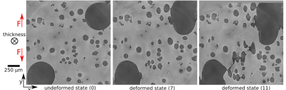
The scanned zone encompasses the two holes. The selected ROI for DVC and FE calculations mainly focuses on the ligament between the two holes (Figure 2(b)). The two machined holes are 500 µm in diameter and the nodule population, which is assumed to behave as voids in the FE computations, has a characteristic diameter of 60 µm. It is considered as secondary void population, which can be observed at micrometer resolutions. Figure 3 shows mid-thickness sections of the reconstructed volume for three different load stages. Classical void coalescence mechanisms are accompanied by sheet coalescence between the two machined holes in the last load-ing step (deformed state (11)).
undeformed state (0) deformed state (7) deformed state (11) x y F F thickness 250 µm
Fig. 3 Mid-thickness section of the reconstructed volume for three different loading steps
2.2 Digital Volume Correlation
Global DVC, which is used herein, is an extension of global 2D DIC [51, 52]. Re-constructed volumes are described by discrete gray level fields of spatial (voxel) coordinate x. DVC consists in registering the gray levels I0in the reference
configu-ration with those of the deformed volume Itsuch that their conservation is obtained
I0(x) = It[x + u(x)] (1)
where u is the Lagrangian displacement field. In experiments gray level conser-vation (1) is never satisfied in laminography due to acquisition noise and recon-struction artifacts [53]. Therefore the gray level residual ρ(x) = I0(x) − It[x + u(x)]
is globally minimized by considering its L2-norm with respect to kinematic un-knowns, which parameterize the measured displacement field. For global DVC, the whole ROI is considered and the global residual Φc2
Φc2({u}) =
∑
ROI
is minimized with respect to the unknown degrees of freedom upgathered in the
column vector {u} when the displacement field is written as u(x, {u}) =
∑
p
upΨΨΨp(x) (3)
where ΨΨΨp(x) are selected displacement fields associated with the parameterization
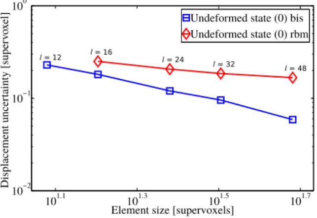
of u(x, {u}). Finite element shape functions are of particular interest since they pro-vide direct links between measured displacement fields and numerical simulations. DVC based on hexahedral finite elements with trilinear shape functions [35] is uti-lized herein. Only a part of the reconstructed volume, which is referred to as DVC ROI, is considered (Figure 2(b)). To keep large ROI sizes, the reconstructed volumes are coarsened (i.e., each 8 neighboring voxels are averaged to form one supervoxel). The measurement uncertainties are quantified by registering two volumes of the unloaded sample (0) with (coined “rbm”) and without (i.e., “bis”) rigid body mo-tion (RBM) applied between acquisimo-tions. Noise and reconstrucmo-tion artifacts make these two volumes non identical. The corresponding displacement fields account for laminography and DVC effects on the measurement uncertainties [54]. The measurement uncertainties are assessed by the standard deviation of displacement fields. Figure 4 shows the standard displacement uncertainties for different element sizes `. Decreasing the element size induces an increase of the displacement un-certainty [55, 56]. The element size used hereafter is set to ` = 16 supervoxels and corresponds to a standard displacement uncertainty of 0.25 supervoxel. This level is the limit below which the estimated displacement levels are no longer trustworthy.
101.1 101.3 101.5 101.7 10−2
10−1
100
Element size [supervoxels]
Displace ment unce rtaint y [super v o x
el] Undeformed state (0) bis Undeformed state (0) rbm
l = 16
l = 24
l = 32 l = 48 l = 12
Fig. 4 Standard displacement uncertainties as functions of the element size ` expressed in super-voxels for two different acquisitions of the reference configuration
Successful DVC registrations were achieved for the first 9 incremental calcula-tions (i.e., registracalcula-tions between step n − 1 and step n). The measured displacement
fields will serve as DVC-FE boundary conditions. The measured displacement fields are interpolated for each loading step onto the FE mesh of the ROI using the shape functions of the DVC mesh).
2.3 Simulations
To perform microscale FE simulations the numerical framework discussed in Refs. [44, 57, 46, 58, 47] is followed. The ROI selected for the FE simulations has to belong to all DVC ROIs for each analyzed loading step and to be made as large as possi-ble [25]. To model the experimental microstructure standard image processing op-erations are carried out [59, 60], namely, smoothing the data, applying a gray value threshold to separate matrix and voids, and then converting these binary data into signed distance function. The latter is interpolated onto a first mesh of uniform size of 10 µm of the FE ROI via trilinear interpolation. The corresponding signed dis-tance function is then regularized with a parallel reinitialization algorithm [46], and used to locate the interfaces [25, 47]. An adaption step is added to control the local maximum curvature of the interface [25, 58]. These different steps are exemplified in Figure 5 for a 2D laminography section. The final mesh has a size of 10 µm close to matrix/void interfaces and 50 µm at a distance of 100 µm from any interface with a linear transition. As shown in Figure 5 the FE discretization of the microstructure is very close to the experimental observation.
The graphite nodules are modeled as zones with very low Young’s modulus [18, 21, 22, 19, 25], while the ferritic matrix is considered as an elastoplastic medium with power law hardening
σ0(p) = σy+ K pn (4)
where p is the equivalent plastic strain, σythe initial yield stress, K the plastic
modu-lus and n the hardening exponent. The properties of the matrix (Table 1) are deduced from tensile experiments on pure ferrite [21].
Table 1 Elastoplastic properties of the ferritic matrix
E(GPa) ν σy(MPa) K (MPa) n
210 0.30 290 382 0.35
The satisfaction of equilibrium equations is obtained with a mixed velocity-pressure formulation solved with P1+/P1 elements to avoid locking [61]. The non-linear behavior of the matrix requires Newton-Raphson schemes to be implemented locally and globally [62]. An updated Lagrangian scheme is used to handle large deformations. Further, large distortions and possible flip of elements are avoided with automatic mesh motion and adaption [47].
Filters and signed distance transform
Trilinear interpolation from image to mesh
and reinitialization Mesh generation and adaption (a) (b) (d) (c) (e) (f) thickness
F
F
250 µmFig. 5 Image immersion and meshing. (a) Initial laminography 2D section. (b) Signed distance function computed thanks to image processing. (c) Signed distance function interpolated and reini-tialized on the FE mesh [46]. (d) Conforming FE mesh generated and adapted to interfaces and local maximum curvature, (e) Zoom on the FE mesh. (f) Comparison between initial laminogra-phy 2D section and interfaces in the final FE mesh (in white)
3 Results
The numerical results using DVC-FE are illustrated in Figure 6. This computation considers 100 voids meshed with ≈ 1 million elements. Void growth and equivalent plastic strains develop as more load is applied.
(a) (b) (c) (d)
F
F
250 µm thicknessFig. 6 ROI calculation results using DVC-FE showing the 3D meshed voids and the equivalent plastic strain on sections when: (a) u = 0 (undeformed state), (b) u = 83.4 µm, (c) u = 192.2 µm, (d) u = 320.8 µm
3.1 Error estimators
Relative displacement comparisons are first reported. Measured displacement fields (via DVC) are applied to the boundaries of the FE ROI. They are also available within the whole ROI. Thus, DVC and DVC-FE displacement fields can be interpo-lated on the same mesh and directly compared as reported in Figure 7. The main dif-ferences are concentrated around debond zones between the matrix and the nodules, while those close to the boundaries are mostly zero. The fact that the differences become significantly larger than the displacement uncertainty is a first indication of model error.
The errors in terms of gray level residuals are now discussed. For each pair of consecutive loading steps, the volume reconstructed for the second step can be de-formed back with the measured or computed displacement field. This corrected vol-ume can be compared voxelwise with the volvol-ume of the first step. With a newly developed tetrahedral-DVC code [63, 38] FE computations with tetrahedral meshes can be imported in the reconstructed volumes frame where the displacement fields
Fig. 7 Mid-section normal to z-direction showing absolute difference between DVC and DVC-FE displacement fields. The displacement difference is expressed in supervoxels
(1 supervoxel ←→ 2.2 µm) x
y
F F
are interpolated voxelwise. The deformed volume It(x) is corrected by the computed
displacement field uFE(x), i.e., It(x + uFE(x)) is obtained. The gray level residuals,
namely, differences between the volume of the reference configuration I0(x) and
the corrected deformed volume It(x + u(x)) are assessed for DVC and FE
com-putations. Quantitative and local error measurements are evaluated for DVC and DVC-FE procedures. Figure 8 shows the standard deviation of residual fields that are normalized by the dynamic range of the volume (i.e., 256 gray levels). The DVC residuals remain close to those observed in the uncertainty analysis for which no strains occurred. Therefore the DVC results are deemed trustworthy.
Displacement [mm] 10.2 47.0 83.4 117.7 152.3 192.2 238.1 280.3 320.8 Standard deviation [%]2.4 2.6 2.8 3 3.2 3.4 3.6 DVC DVC-FE DVC uncert. bis
Fig. 8 Standard deviation for the dimensionless gray level residual fields for all loading steps. For comparison purposes, the dashed line corresponds to the uncertainty analysis for the so-called “bis” case (see Subsection 2.2)
The errors produced by the micromechanical models inside the DVC-FE domain also remain low and slightly increase at later loading steps (from ≈ 15% initially to ≈ 20% in last loading step). However they are always higher than the DVC residuals. This observation confirms model errors that become more significant as coalescence sets in. Figure 9 confirms that these differences between DVC-FE simulations and experiments are mostly concentrated around interfaces.
100 200 300 50 100 150 200 0 20 40 60 80 x y (a) DVC 100 200 300 50 100 150 200 0 20 40 60 80 x y (b) DVC-FE
Fig. 9 Absolute gray level differences at the z midsection after correction with DVC (a) and DVC-FE (b) displacements for the ninth loading step
3.2 Damage analysis
Damage predictions of DVC-FE are qualitatively compared studying the x-midsection of the ROI with experimental images in Figure 10. Since measured boundary
condi-(a) (b) (c) (d) thickness
F
F
250 µmFig. 10 ROI (blue line) calculation results using DVC-FE comparing the numerical matrix/void interface (white line) with experimental images for the x-midsection. (a) u = 0 (undeformed state), (b) u = 83.4 µm, (c) u = 192.2 µm, (d) u = 320.8 µm
tions are expected to follow experimental images at the spatial resolution of DVC, the matrix/void interfaces in the simulation (in white in the figure) are superim-posed. The interfaces are very accurately meshed on average and tracked during the simulation up to the last loading step. Quantitatively void growth is defined by
f =void volume
ROI volume , void growth = f f0
(5)
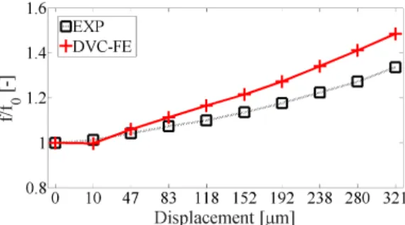
where f0is the initial void volume fraction. Void growth plots are shown in
Fig-ure 11 in which the ‘EXP’ curve is obtained in processed laminography volumes (i.e., images with smooth signed distance functions as shown in Figure 5(b)).
Fig. 11 Void volume change observed experimentally and predicted within the present framework
The numerical results show a small decrease of porosity p at the first loading step. This is not observed experimentally. This first loading step is bigger than the subsequent ones, which asks for extensive remeshing in the computations. Conse-quently interfaces are slightly smoothened and void volume can be diffused. For the other loading steps, void growth is overestimated numerically. This may be due to the fact that nodules are considered as very soft media in the computations, while in reality only the voids grow after nodule/matrix interface debonding (Figure 10).
4 Discussion
Although the results using DVC-FE look very promising, several issues need to be addressed. There still are gaps between FE-DVC and DVC results (see Figures 9 and 10). This gap increases when reaching the final loading steps. Similarly, the displacement difference (Figure 7) is significantly higher than the displacement un-certainty reported in Figure 4. The differences are mainly concentrated around ma-trix/nodule interfaces. This observation calls for better models of the nodules and interface debonding. Further, the increase of the error at later loading steps proves the inability of the constitutive law used for the ferritic matrix to fully capture the acceleration of void growth and subsequent coalescence. Better calibrated and more
advanced plasticity models may be considered at the microscale to better capture the multiscale plastic flow. These additional developments will extensively rely on DVC-FE and its ability to provide experimentally measured boundary conditions for micromechanical simulations. The extension of Integrated-DVC to 4D analyses [38] will be utilized to conduct inverse analyses based on these error measurements and calibrate material parameters at the microscale.
Acknowledgements This work was performed within the COMINSIDE project funded by the French Agence Nationale de la Recherche (ANR-14-CE07-0034-02 grant). We also acknowledge the European Synchrotron Radiation Facility for provision of beamtime at beamline ID15, experi-ment ME 1366. It is also a pleasure to acknowledge the support of BPI France (“DICCIT” project), and of the Carnot M.I.N.E.S institute (“CORTEX” project). M. Kuna and L. Zybell from IMFD, TU Freiberg, are thanked for materials supply and machining as well as for scientific discussions.
References
1. L. Kachanov, Bull. SSR Acad. Sci., Division of Technical Sciences (in Russian) 8, 26 (1958) 2. Y. Rabotnov, On the Equations of State for Creep (McMillan, New York (USA), 1963), pp.
307–315
3. J. Lemaitre, A Course on Damage Mechanics (Springer-Verlag, Berlin (Germany), 1992) 4. T.S. Cao, E. Maire, C. Verdu, C. Bobadilla, P. Lasne, P. Montmitonnet, P.-O. Bouchard,
Com-put. Mat. Sci. 84, 175 (2014)
5. T.S. Cao, C. Bobadilla, P. Montmitonnet, P.-O. Bouchard, J. Mat. Proc. Technol. 216, 385 (2015)
6. A. Gurson, ASME J. Eng. Mat. Techn. 99, 2 (1977)
7. A. Needleman, V. Tvergaard, J. Mech. Phys. Solids 32(6), 461 (1984) 8. M. Geers, R. De Borst, T. Peijs, Compos. Sci. Tech. 59, 1569 (1999) 9. D. Claire, F. Hild, S. Roux, C. R. M´ecanique 330, 729 (2002) 10. S. Roux, F. Hild, Exp. Mech. 48(4), 495 (2008)
11. L. Babout, Y. Br´echet, E. Maire, R. Foug`eres, Acta Mat. 52(15), 4517 (2004)
12. P.-O. Bouchard, L. Bourgeon, H. Lachap`ele, E. Maire, C. Verdu, R. Forestier, R. Log´e, Mat. Sci. Eng. A 496(1-2), 223 (2008)
13. T. Ueda, L. Helfen, T.F. Morgeneyer, Acta Mat. 78, 254 (2014)
14. F. Hannard, T. Pardoen, E. Maire, C. Le Bourlot, R. Mokso, A. Simar, Acta Mat. 103, 558 (2016)
15. T. Morgeneyer, T. Taillandier-Thomas, A. Buljac, L. Helfen, F. Hild, J. Mech. Phys. Solids 96, 550 (2016)
16. T. Morgeneyer, J. Besson, H. Proudhon, M. Starink, I. Sinclair, Acta Mat. 57(13), 3902 (2009) 17. S. Tang, A.M. Kopacz, S. Chan O’Keeffe, G.B. Olson, W.K. Liu, J. Mech. Phys. Solids 61(11),
2108 (2013)
18. M.J. Dong, C. Prioul, D. Franc¸ois, Metall. Mat. Trans. A 28(11), 2245 (1997) 19. G. H¨utter, L. Zybell, M. Kuna, Eng. Fract. Mech. 144, 118 (2015)
20. Z. Tomiˇcevi´c, J. Kodvanj, F. Hild, European Journal of Mechanics - A/Solids 59, 140 (2016) 21. K. Zhang, J. Bai, D. Franc¸ois, Int. J. Solids Struct. 36(23), 3407 (1999)
22. N. Bonora, A. Ruggiero, International Journal of Solids and Structures 42(5-6), 1401 (2005) 23. G. H¨utter, L. Zybell, U. M¨uhlich, M. Kuna, Comput. Mat. Sci. 80, 61 (2013)
24. G. H¨utter, L. Zybell, M. Kuna, Int. J. Solids Struct. 51(3-4), 839 (2014)
25. A. Buljac, M. Shakoor, J. Neggers, L. Helfen, M. Bernacki, P.-O. Bouchard, T.F. Morgeneyer, F. Hild, Computational Mechanics (2017). DOI 10.1007/s00466-016-1357-0
26. L. Helfen, A. Myagotin, P. Pernot, M. DiMichiel, P. Mikul´ık, A. Berthold, T. Baumbach, Nucl. Inst. Meth. Phys. Res. B 563, 163 (2006)
27. L. Helfen, T. Morgeneyer, F. Xu, M. Mavrogordato, I. Sinclair, B. Schillinger, T. Baumbach, Int. J. Mat. Res. 2012(2), 170 (2012)
28. V. Maurel, L. Helfen, F. N’Guyen, A. K¨oster, M. Di Michiel, T. Baumbach, T. Morgeneyer, Scripta Mat. 66, 471 (2012)
29. D. Bull, S. Spearing, I. Sinclair, L. Helfen, Compos. Part A 52, 62 (2013)
30. P. Reischig, L. Helfen, A. Wallert, T. Baumbach, J. Dik, Apply. Phys. A 111, 983 (2013) 31. B. Bay, T. Smith, D. Fyhrie, M. Saad, Exp. Mech. 39, 217 (1999)
32. T. Smith, B. Bay, M. Rashid, Exp. Mech. 42(3), 272 (2002)
33. M. Bornert, J. Chaix, P. Doumalin, J. Dupr´e, T. Fournel, D. Jeulin, E. Maire, M. Moreaud, H. Moulinec, Inst. Mes. M´etrol. 4, 43 (2004)
34. E. Verhulp, B. van Rietbergen, R. Huiskes, J. Biomech. 37(9), 1313 (2004) 35. S. Roux, F. Hild, P. Viot, D. Bernard, Comp. Part A 39(8), 1253 (2008)
36. J. Rannou, N. Limodin, J. R´ethor´e, A. Gravouil, W. Ludwig, M. Ba¨ıetto, J. Buffi`ere, A. Combescure, F. Hild, S. Roux, Comp. Meth. Appl. Mech. Eng. 199, 1307 (2010) 37. A. Bouterf, S. Roux, F. Hild, J. Adrien, E. Maire, Strain 50(5), 444 (2014)
38. F. Hild, A. Bouterf, L. Chamoin, F. Mathieu, J. Neggers, F. Pled, Z. Tomiˇcevi´c, S. Roux, Adv. Mech. Simul. Eng. Sci. 3(1), 1 (2016)
39. Y. Zhang, C. Bajaj, B.S. Sohn, Comput. Meth. Appl. Mech. Eng. 194(48-49), 5083 (2005) 40. P.G. Young, T.B.H. Beresford-West, S.R.L. Coward, B. Notarberardino, B. Walker, A.
Abdul-Aziz, Phil. Trans. A 366(1878), 3155 (2008)
41. S. Osher, J.A. Sethian, J. Comput. Phys. 79(1), 12 (1988)
42. R. Kimmel, D. Shaked, N. Kiryati, A.M. Bruckstein, Comput. Vis. Image Underst. 62(3), 382 (1995)
43. N. Sukumar, D. Chopp, N. Mo¨es, T. Belytschko, Comput. Meth. Appl. Mech. Eng. 190(46-47), 6183 (2001)
44. E. Roux, M. Bernacki, P.-O. Bouchard, Comput. Mat. Sci. 68, 32 (2013)
45. D.L. Quan, T. Toulorge, E. Marchandise, J.F. Remacle, G. Bricteux, Comp. Meth. Appl. Mech. Eng. 268, 65 (2014)
46. M. Shakoor, B. Scholtes, P.-O. Bouchard, M. Bernacki, Appl. Math. Model. 39(23-24), 7291 (2015)
47. M. Shakoor, P.-O. Bouchard, M. Bernacki, Int. J. Num. Meth. Eng. (2016). DOI 10.1002/nme.529
48. A. Weck, D. Wilkinson, Acta Materialia 56(8), 1774 (2008)
49. A. Myagotin, A. Voropaev, L. Helfen, D. H¨anschke, T. Baumbach, IEEE Trans. Image Process. 22(12), 5348 (2013)
50. M. Vogelgesang, T. Farago, T.F. Morgeneyer, L. Helfen, T. dos Santos Rolo, A. Myagotin, T. Baumbach, J. Synchrotron Rad. 23, 1254 (2016)
51. G. Besnard, F. Hild, S. Roux, Exp. Mech. 46, 789 (2006) 52. F. Hild, S. Roux, Exp. Mech. 52(9), 1503 (2012)
53. F. Xu, L. Helfen, T. Baumbach, H. Suhonen, Optics Exp. 20, 794 (2012) 54. T. Morgeneyer, L. Helfen, H. Mubarak, F. Hild, Exp. Mech. 53(4), 543 (2013)
55. N. Limodin, J. Rthor, J. Adrien, J. Buffire, F. Hild, S. Roux, Exp. Mech. 51(6), 959 (2011) 56. H. Leclerc, J. P´eri´e, F. Hild, S. Roux, Mech. & Indust. 13, 361 (2012)
57. E. Roux, M. Shakoor, M. Bernacki, P.-O. Bouchard, Model. Simul. Mat. Sci. Eng. 22(7), 075001 (2014)
58. M. Shakoor, M. Bernacki, P.-O. Bouchard, Eng. Fract. Mech. 147, 398 (2015)
59. J. Schindelin, I. Arganda-Carreras, E. Frise, V. Kaynig, M. Longair, T. Pietzsch, S. Preibisch, C. Rueden, S. Saalfeld, B. Schmid, J.Y. Tinevez, D.J. White, V. Hartenstein, K. Eliceiri, P. Tomancak, A. Cardona, Nature Meth. 9(7), 676 (2012)
60. C.A. Schneider, W.S. Rasband, K.W. Eliceiri, Nature Meth. 9(7), 671 (2012)
61. D. Boffi, F. Brezzi, L.F. Demkowicz, R.G. Dur´an, R.S. Falk, M. Fortin, Mixed Finite Ele-ments, Compatibility Conditions, and Applications, Lecture Notes in Mathematics, vol. 1939 (Springer Berlin Heidelberg, Berlin, Heidelberg, 2008)
62. R.H. Wagoner, J.L. Chenot, Metal Forming Analysis (Cambridge University Press, 2001)
63. H. Leclerc, J. Neggers, F. Mathieu, S. Roux, F. Hild, Correli 3.0.
IDDN.FR.001.520008.000.S.P.2015.000.31500, Agence pour la Protection des Programmes, Paris (France) (2015)