HAL Id: tel-01952827
https://tel.archives-ouvertes.fr/tel-01952827
Submitted on 12 Dec 2018HAL is a multi-disciplinary open access archive for the deposit and dissemination of sci-entific research documents, whether they are pub-lished or not. The documents may come from teaching and research institutions in France or abroad, or from public or private research centers.
L’archive ouverte pluridisciplinaire HAL, est destinée au dépôt et à la diffusion de documents scientifiques de niveau recherche, publiés ou non, émanant des établissements d’enseignement et de recherche français ou étrangers, des laboratoires publics ou privés.
geotechnical engineering within the framework of
micropolar theory
Jiangxin Liu
To cite this version:
Jiangxin Liu. Numerical investigations of the strain localization in geotechnical engineering within the framework of micropolar theory. Civil Engineering. École centrale de Nantes, 2018. English. �NNT : 2018ECDN0005�. �tel-01952827�
Jiangxin
LIU
JURYPrésident : MILLET Olivier
Rapporteurs : SHAO Jianfu, Professeur des Universités, Université des Sciences et Technologies de Lille 1 LAOUAFA Farid, Ingénieur (HDR), INERIS
Examinateurs : MILLET Olivier, Professeur des Universités, Universités de la Rochelle PAPON Aurélie, Maître de conférences, INSA Toulouse
Directeur de thèse : YIN Zhenyu, Maître de conférences (HDR), Ecole Centrale de Nantes Co-directeur de thèse : HICHER Pierre-Yves, Professeur Émérite, Ecole Centrale de Nantes
Mémoire présenté en vue de lʼobtention
du grade de Docteur de lʼEcole Centrale de Nantes Sous le label de l’UNIVERSITÉ BRETAGNE LOIRE
École doctorale : Sciences pour l'Ingénieur
Discipline : Génie Civil
Unité de recherche : Institut de recherche en génie civil et mécanique
Soutenue le 22 Mars 2018
Etude numérique de la localisation des déformations en
géotechnique dans le cadre de la théorie micropolaire
I
II
This research was motivated, supervised and strongly supported by my advisors Dr. Zhenyu YIN and Prof. Pierre-Yves HICHER. Their insight, encouragement, dedication, and great personality helped me throughout this research. I am greatly thankful for both of them.
Moreover, I would like to thank the faculty who contributed to this in accepting to serve in my PhD committee, Prof. Olivier MILLET, Prof. Jianfu SHAO, Dr. LAOUAFA Farid and Dr. Aurélie PAPON; I appreciate their help and fruitful discussions. I would like to express sincere thanks to my language teacher SHIMU, who always encourages me to speak French and corrects my grammar mistakes in my manuscripts. I would like also to thank the Chinese friends Zheng LI, Jian LI, Yinfu JIN, Chaofa ZHAO, Zexiang WU, Jie YANG…, for their valuable discussions and cooperations. The help and care from Ran ZHU, Zhuang JIN, Huang WANG and Kexin YIN are also worth appreciating. Special thanks for Prof. Wenxiong HUANG for his valuable discussions. I would like to thank my officemates Benoit, George and Reda for their support and patience.
I feel very much indebted to my parents, my sisters and my wife for their love, support and endurance. I also thank my daughter Amira who makes me a caring, patient and persistent man.
Last, I want to appreciate the friendship between China and France, and I would acknowledge the financial support from China Scholarship Council.
III
Most of the progressive failures of geotechnical structures are associated with the strain localization phenomenon, which is generally accompanied by strength softening. Many experimental observations show that significant rearrangements and rotations of particles occur inside the shear bands. The aim of this thesis is to investigate numerically the strain localization phenomena of granular materials. Considering the mesh dependency problems in finite element analysis caused by strain softening within the classical continuum framework, a sand model based on critical-state has been formulated within the framework of the micropolar theory, taking into account the micro rotations, and implemented into a finite element code for two dimensional problems. Then, the simulations of the shear band in biaxial tests are comprehensively studied in terms of onset, thickness, orientation, etc. At the same time, the efficiency of the micropolar approach, as a regularization technique, is discussed. This is followed by an instability analysis using the second-order work based on the micropolar continuum theory. Finally, for a wider application in simulating failures in geotechnical engineering, the 2D model has been extended to 3D model. Based on the entire study, both the 2D and 3D model demonstrate obvious regularization ability to relieve the mesh dependency problems and to reproduce reasonably the shear bands in geostructures.
Key words: Granular soils, shear band, finite element method, mesh dependency, micropolar theory,
IV
La plupart des défaillances des structures géotechniques sont associées aux phénomènes de localisation des déformations, qui s'accompagnent toujours d'un adoucissement de la résistance. De nombreuses observations expérimentales montrent que d’importants réarrangements et rotations de particules se produisent à l'intérieur des bandes de cisaillement. Cette thèse vise à étudier numériquement les phénomènes de localisation des déformations dans les matériaux granulaires. Considérant les problèmes de dépendance au maillage dans l'analyse par éléments finis dans le cadre de la modélisation continue classique, un modèle de sable basé sur l'état critique a été formulé dans le cadre de la théorie micropolaire. Un code d'élément pour les problèmes bidimensionnels a été développé dans ce cadre. Ensuite, les simulations d’essais biaxiaux ont permis d’étudier en profondeur les caractéristiques des bande de cisaillement en termes d'apparition, d'épaisseur et d'orientation, etc… Dans le même temps, l'efficacité de l'approche micropolaire, en tant que technique de régularisation, a été discutée. L'analyse de l'instabilité dans un continuum micropolaire basé sur le travail du second ordre a également été effectuée. Enfin, pour une application plus large dans la simulation des défaillances en ingénierie géotechnique, le modèle 2D a été étendu à un modèle 3D. Sur la base de l'étude, les modèles 2D et 3D ont démontré leurs capacités de régularisation pour éviter les problèmes de dépendance au maillage et reproduire raisonnablement la bande de cisaillement dans les géostructures.
Mots-clés: Sol granulaire, bande de cisaillement, méthode des éléments finis, dépendance au
i
Acknowledgments... II Abstract ... III Résume ... IV Table content ... i List of figures ... v
List of tables ... xiii
General introduction ... 1
Introduction générale ... 3
Chapter 1 Literature Survey ... 5
1.1 Introduction ... 5
1.2 Strain localization phenomena ... 6
1.2.1 Engineering scale: collapse of geotechnical structures ... 6
1.2.2 Model scale: strain localization in model tests ... 9
1.2.3 Laboratory sample scale: strain localization in specimens ... 12
1.3 Mechanisms of strain localization ... 14
1.4 Theories and methods of describing strain localization ... 17
1.4.1 Experimental investigations ... 17
1.4.2 Constitutive models and theories ... 25
1.4.3 Numerical analysis ... 27
1.4.4 Non–localized regularization approaches ... 31
1.5 Application of micropolar theory in geotechnical engineering... 46
1.5.1 Different polarized constitutive models and the applications ... 46
1.5.2 Internal length scale and micropolar shear modulus ... 48
1.6 Conclusions ... 51
Chapter 2 Finite Element Implementation of the Micropolar SIMSAND Model ... 52
ii
2.2.1 Description of SIMSAND model... 53
2.2.2 Extension to the micropolar SIMSAND model ... 56
2.2.3 Summary of model parameters ... 59
2.3 Finite element implementation ... 61
2.3.1 Formulations of UEL ... 61
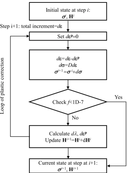
2.3.2 Integration algorithm-cutting plane method ... 68
2.3.3 Numerical validations ... 73
2.4 Verification of the micropolar model with plane strain tests results ... 76
2.5 Numerical simulations of shear bands in biaxial tests ... 80
2.5.1 Mesh dependency of the simulated results by classical SIMSAND model ... 81
2.5.2 Mesh independency of the simulated results by micropolar SIMSAND model ... 84
2.6 Application of the micropolar model in simulating retaining wall ... 86
2.6.1 Mesh dependency of the simulated results by classical SIMSAND model ... 87
2.6.2 Mesh independency of the simulated results by micropolar SIMSAND model ... 90
2.7 Conclusions ... 93
Chapter 3 Numerical Analysis of Shear Band ... 94
3.1 Introduction ... 94
3.2 Numerical investigation of shear band by micropolar approach ... 94
3.2.1 Mechanical response ... 94
3.2.2 Shear band inclination ... 95
3.2.3 Shear band thickness and shear band identifications ... 97
3.2.4 Shear band evolution ... 100
3.2.5 Influence of internal length on the simulated results ... 101
3.2.6 Influences of the micropolar shear modulus ... 106
3.3 Some other advantages of the micropolar approach ... 112
3.4 Proposition of the regularization effectiveness ratio—lc⁄le ... 117
3.5 Influencing factors on shear band and regularization effectiveness ratio ... 124
iii
3.5.3 Influence of several key parameters ... 128
3.6 Conclusions ... 133
Chapter 4 Second-Order Work Criterion in Micropolar Theory ... 135
4.1 Introduction ... 135
4.2 Mathematical implications of instability ... 136
4.2.1 Material instability ... 136
4.2.2 Structural instability ... 139
4.2.3 Second-order work framework ... 141
4.3 Formulations of second-order work in micropolar theory ... 142
4.3.1 General equation of second-order work ... 142
4.3.2 Second-order work in classical continuum theory based FE analysis ... 143
4.3.3 Second-order work in micropolar theory based FE analysis ... 143
4.4 Discussions of second-order work in FE analysis by simulating a biaxial test ... 144
4.4.1 Second-order work behind the mechanical response ... 145
4.4.2 Comparisons of second-order work from classical model and polarized model ... 146
4.4.3 Mesh dependency analysis of classical model by the second-order work ... 148
4.4.4 Mesh independency analysis of micropolar model by the second-order work ... 150
4.4.5 Discussions of the contribution of micro rotations to the second-order work ... 153
4.5 Application of the second-order work in the analysis of a retaining wall ... 155
4.6 Conclusions ... 157
Chapter 5 Extension of the micropolar model from 2D to 3D ... 159
5.1 Introduction ... 159
5.2 Framework of the 3D micropolar theory ... 159
5.2.1 Equilibrium formulations ... 159
5.2.2 Kinematics formulations ... 163
5.2.3 Force stress and moment stress of a micropolar continuum ... 166
5.2.4 Constitutive equations for a micropolar elasticity ... 167
iv
5.3.2 Kinematics equations ... 169
5.3.3 Finite element discretization ... 169
5.4 FE implementation of the 3D critical state–based micropolar model ... 172
5.5 Numerical simulations and discussions ... 175
5.5.1 Element validation ... 175
5.5.2 Boundary value problems in plane strain condition ... 178
5.5.3 Boundary value problems in a real 3D condition ... 185
5.6 Conclusions ... 188
Conclusions and Perspectives ... 190
Conclusions ... 190
Perspectives... 191
Appendix A: Numerical Pathological Solutions ... 192
Ill-posedness of static loading problems ... 192
Ill-posedness of dynamic loading problems ... 193
Appendix B: Mesh Dependency Problem within Classical Continuum Theory ... 195
Appendix C: Full Formulations of Micropolar Theory ... 198
Equilibrium equations ... 200 Static equilibrium ... 200 Dynamic equilibrium ... 202 Kinematics equations ... 204 Constitutive laws ... 206 Elastic models ... 206 Elastoplastic models... 207
Appendix D: Brief Introduction of UMAT and Validation ... 209
Introduction of UMAT ... 209
Verification of UMAT ... 210
Appendix E: Calibration with Optimization Method ... 214
v
List of figures
Figure 1-1 Uneven settlement and the collapse of buildings: (a) Tower of Pisa; (b) residential
buildings in Shanghai ... 6
Figure 1-2 Collapse of typical geotechnical structures: (a) landslide in San Salvador; (b) slide of a high embankment; (c) collapse of the excavation surface; (d) failure of a retaining wall ... 7
Figure 1-3 Major types of failure of slope: (a) rotational landslide; (b) translational landslide; (c) block slide ... 8
Figure 1-4 Centrifuge and typical centrifuge modellings. (a) Centrifuge machine (b) Dike model (c) Uneven settlement (d) Street pile wall ... 10
Figure 1-5 Progressive failure of retaining wall by geo-hazard tank model: (a) initial state; (b) formation of first shear band; (c) formation of several shear band; (d) collapse of soil ... 11
Figure 1-6 Soil failure under footing by geo-hazard tank model: (a) initial state; (b) formation of the triangle area under footing; (c) laterally uplift outward; (d) formation of slide surface ... 12
Figure 1-7 Apparatus and specimens: (a) triaxial test; (b) biaxial test ... 14
Figure 1-8 Stress and strain of the specimen in triaxial or biaxial test ... 15
Figure 1-9 Investigations of shear band with computed tomography technique: (a) observation of Desrues; (b) observation of Alshibli; (c) observation of Bésuelle ... 19
Figure 1-10 DEM simulations of shear band in: (a) biaxial test; (b) simple shear test ... 29
Figure 1-11 Standard procedure of Finite Element Analysis ... 30
Figure 1-12 One-dimensional viscoplastic model for example ... 33
Figure 1-13 Spatial average: (a) profiles of micro strain and average strain along a segment with point x in the center of a representative volume; (b) sketch of the representative volume with the center point x; (c) the representative volume near the surface of the body; (d) the weighting function for non-local averaging integral and its relation to the internal length scale l ... 36
Figure 1-14 Typical evolution of plastic strain distribution in strain localization of softening materials ... 39 Figure 1-15 Separation between micro-rotation and macro-rotation in 2D space and their effect in the
vi
Figure 2-1 Principle of critical-state-based nonlinear hardening model for sand ... 56
Figure 2-2 Subroutine interface of UEL ... 62
Figure 2-3 Flow chart of the UEL ... 63
Figure 2-4 Element of 2D micropolar continuum: (a) 8-node plane element; (b) integration points .. 64
Figure 2-5 Illustration of correction phase of cutting plane algorithm ... 70
Figure 2-6 Flow chart of iteration procedure of the cutting plane algorithm ... 72
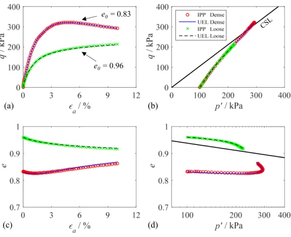
Figure 2-7 Comparisons between IPP and UEL in simulating biaxial drained tests ... 75
Figure 2-8 Comparisons between IPP and UEL in simulating biaxial undrained tests ... 75
Figure 2-9 Comparison between experimental and simulated shear band for very dense sand under 100 kPa confining pressure at 10% axial strain: (a) experimental biaxial test; (b) simulated results with the micropolar model ... 78
Figure 2-10 Comparisons between the simulated solutions and experimental data for medium dense F-75 sand: (a) axial strain versus principle stress ratio; (b) axial strain versus volumetric strain 79 Figure 2-11 Comparisons between the simulated solutions and experimental data for very dense F-75 sand: (a) axial strain versus principle stress ratio; (b) axial strain versus volumetric strain ... 80
Figure 2-12 Shear bands of four different mesh sizes using the classical model: (a) mesh 10×20; (b) mesh 15×30; (c) mesh 20×40; (d) mesh 30×60 ... 82
Figure 2-13 Load–displacement of four different mesh sizes using the classical model ... 82
Figure 2-14 Shear band orientation of different meshes (a) mesh 10×20 1=52.69°; (b) mesh 15×30 2=57.65°; (c) mesh 20×40 3=60.15° ... 83
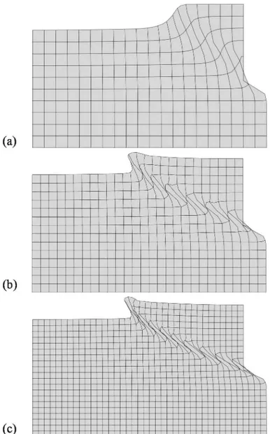
Figure 2-15 Shear bands of four different mesh sizes using the micropolar model: (a) mesh 10×20; (b) mesh 15×30; (c) mesh 20×40; (d) mesh 30×60 ... 84
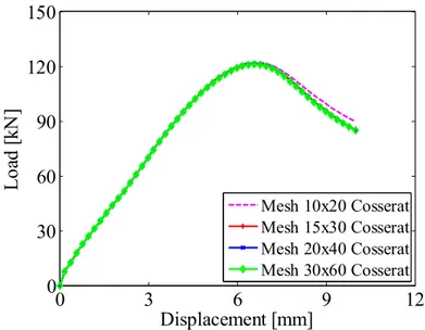
Figure 2-16 Load–displacement of four different mesh sizes based on micropolar model ... 85
Figure 2-17 Shear band orientation of different mesh: (a) mesh 10×20 1=53.10°; (b) mesh 15×30 2=53.22°; (c) mesh 20×40 3=53.22°; (d) mesh 30×60 4=53.22° ... 86
Figure 2-18 A small scale retaining wall model in passive condition ... 87
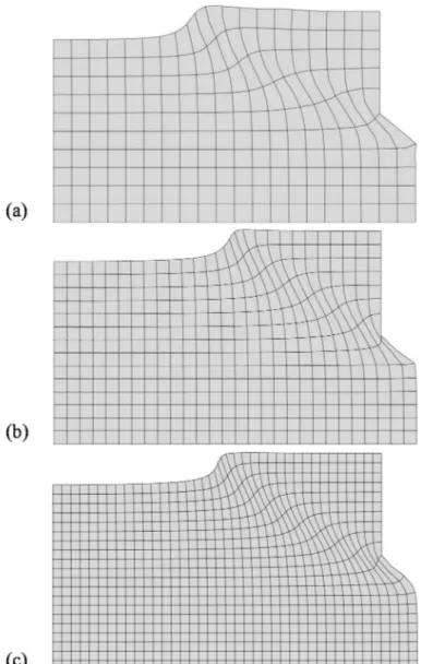
Figure 2-19 The deformation of different meshes by classical model: (a) mesh 20×10; (b) mesh 28×14; (c) mesh 40×20; ... 88
vii
mesh 28×14; (c) mesh 40×20; ... 89
Figure 2-21 The void ratio for different meshes by micropolar model: (a) mesh 20×10; (b) mesh 28×14; (c) mesh 40×20; ... 89
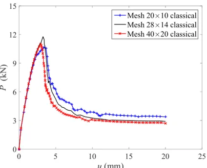
Figure 2-22 Passive load-displacement curves of the retaining wall from classical model ... 90
Figure 2-23 The deformation of different meshes by micropolar model: (a) mesh 20×10; (b) mesh 28×14; (c) mesh 40×20; ... 91
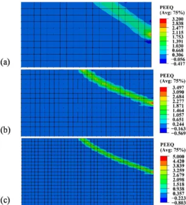
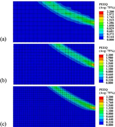
Figure 2-24 The equivalent plastic strain for different meshes by micropolar model: (a) mesh 20×10; (b) mesh 28×14; (c) mesh 40×20; ... 92
Figure 2-25 The void ratio for different meshes by micropolar model: (a) mesh 20×10; (b) mesh 28×14; (c) mesh 40×20; ... 92
Figure 2-26 Passive load-displacement curves of the retaining wall from micropolar model ... 93
Figure 3-1 Comparisons of load–displacement curves of four different mesh sizes between classical model and micropolar model ... 95
Figure 3-2 Volumetric strain versus shear strain ... 96
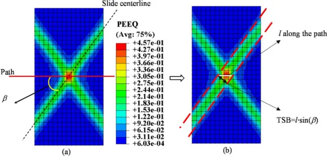
Figure 3-3 Identification of shear band thickness by equivalent plastic strain: (a) selected path and shear band orientation; (b) calculation of the shear band thickness ... 98
Figure 3-4 Shear band thickness identified by different variables ... 99
Figure 3-5 Normalized shear band thickness of four different mesh sizes ... 100
Figure 3-6 Evolution of a shear band ... 100
Figure 3-7 Influence of internal length scale lc on load–displacement curves ... 101
Figure 3-8 Influence of internal length scale lc on shear band orientation: (a) lc = 1 mm, 1 = 55.9°; (b) lc = 1.5 mm, 2 = 54.2°; (c) lc = 2 mm, 3 = 53.2° ... 102
Figure 3-9 Normalized shear band thickness of different lc: (a) based on plastic strain along the selected horizontal path; (b) based on normalized plastic strain along the selected horizontal path ... 103
Figure 3-10 Relationship between thickness of shear band and micro structural size ... 105
Figure 3-11 Normalized shear band thickness versus mean grain size or internal length scale ... 105
viii
Figure 3-14 Influence of micropolar shear modulus Gc on shear band orientation: (a) Gc = 0.5G,
1=53.22°; (b) Gc = 1.0G, 2=53.22°; (c) Gc = 2.0G, 3=53.22° ... 108
Figure 3-15 Influence of micropolar shear modulus Gc on shear band thickness ... 109
Figure 3-16 Influence of micropolar shear modulus Gc on shear strain ... 110
Figure 3-17 Influence of micropolar shear modulus Gc on shear stress ... 110
Figure 3-18 Influence of micropolar shear modulus Gc on micro-curvature ... 111
Figure 3-19 Influence of micropolar shear modulus Gc on micro-moment ... 111
Figure 3-20 Evolution of shear band based on the particles’ rotations: (a) shear band onset corresponding to axial strain 2.5%; (b) corresponding to axial strain 3%; (c) fully formed shear band corresponding to axial strain 5% ... 112
Figure 3-21 Shear bands for different discretization obtained from the classical model for loose materials: (a) mesh 10×20; (b) mesh 15×30; (c) mesh 20×40; (d) mesh 30×60 ... 114
Figure 3-22 Load–displacement curves for different discretization based obtained from the classical model for loose materials ... 114
Figure 3-23 Load–displacement curves of each element from the classical simulation: (a) elements located on the horizontal profile; (b) local–displacement curves of each element ... 115
Figure 3-24 Diffusion mode for different discretization obtained from the micropolar model for loose materials: (a) mesh 10×20; (b) mesh 15×30; (c) mesh 20×40; (d) mesh 30×60 ... 116
Figure 3-25 Load–displacement curves for different discretization based on micropolar model for loose materials ... 116
Figure 3-26 Load–displacement curves of each element from the Cosserat simulation: (a) elements located on the horizontal profile; (b) local–displacement curves of each element ... 117
Figure 3-27 Shear bands for different discretization by the micropolar model with lc = 1 mm: (a) 10×20 mesh; (b) 15×30 mesh; (c) 20×40 mesh; (d) 30×60 mesh ... 120
Figure 3-28 Load–displacement curves for different discretization using the micropolar model: lc = 1 mm ... 121
Figure 3-29 Shear bands for different discretization by the micropolar model with lc = 1.5mm: (a) mesh 10×20; (b) mesh 15×30; (c) mesh 20×40; (d) mesh 30×60 ... 121
ix
... 122 Figure 3-31 Shear bands for different discretization by the micropolar model with lc = 2mm: (a) mesh
10×20; (b) mesh 15×30; (c) mesh 20×40; (d) mesh 30×60 ... 122 Figure 3-32 Load–displacement curves for different discretization by micropolar model: lc=2mm . 123
Figure 3-33 Shear bands for different discretization by the micropolar model with lc = 2.25mm: (a)
mesh 10×20; (b) mesh 15×30; (c) mesh 20×40; (d) mesh 30×60 ... 123 Figure 3-34 Load–displacement curves for different discretization by micropolar model: lc=2.25mm
... 124 Figure 3-35 Influence of confining pressure on the load-carrying capacity ... 126 Figure 3-36 Influence of confining pressure on shear band thickness: (a) based on plastic strain; (b) based on normalized plastic strain ... 126 Figure 3-37 Influence of initial density on the load carrying capacity ... 127 Figure 3-38 Influence of density on shear band thickness: (a) based on plastic strain; (b) based on normalized plastic strain ... 128 Figure 3-39 Influence of critical friction angle u on the load carrying capacity ... 129
Figure 3-40 Influence of critical friction angle u on shear band thickness: (a) based on plastic strain; (b)
based on normalized plastic strain ... 130 Figure 3-41 Influence of strength parameter np on the load carrying capacity ... 131
Figure 3-42 Influence of strength parameter np on shear band thickness: (a) based on plastic strain; (b)
based on normalized plastic strain ... 131 Figure 3-43 Influence of deformation parameter nd on the load carrying capacity ... 133
Figure 3-44 Influence of deformation parameter nd on shear band thickness: (a) based on plastic strain;
(b) based on normalized plastic strain ... 133 Figure 4-1 Order of instability criteria during loading history for non-symmetric constitutive matrices ... 139 Figure 4-2 Definition of particles in contact ... 144 Figure 4-3 Second-order work behind the mechanical response ... 145 Figure 4-4 Comparisons of the results from classical SIMSAND model and the polarized model .. 146
x
4 mm; (b) vertical displacement of 4.5 mm; (c) vertical displacement of 5 mm; (d) vertical
displacement of 5.8 mm ... 147
Figure 4-6 Evolution of the second-order work in the micropolar continuum: (a) vertical displacement of 5.5 mm; (b) vertical displacement of 6 mm; (c) vertical displacement of 7 mm; (d) vertical displacement of 10mm ... 148
Figure 4-7 Instability regions identified by second-order work of different meshes in classical continuum: (a) mesh 10×20; (b) mesh 15×30; (c) mesh 20×40; (d) mesh 30×60 ... 149
Figure 4-8 Comparisons of different meshes in a classical continuum: (a) mechanical responses; (b) evolutions of the second-order work ... 150
Figure 4-9 Instability regions identified by second-order work of different meshes in micropolar continuum: (a) mesh 15×30; (b) mesh 20×40; (c) mesh 30×60 ... 151
Figure 4-10 Comparisons of different meshes in a micropolar continuum: (a) mechanical responses; (b) evolutions of the second-order work ... 152
Figure 4-11 Contribution of the grains rotations to the second-order work ... 153
Figure 4-12 Selecting an element for local analysis of the components of the second-order work .. 154
Figure 4-13 Components of the second-order work of a local element ... 154
Figure 4-14 Components of the global second-order work ... 155
Figure 4-15 Failure zone of the soil mass behind the wall identified by the vanishing of the second-order work of different mesh sizes in a classical continuum: (a) mesh 20×10; (b) mesh 28×14; (c) mesh 40×20 ... 156
Figure 4-16 Failure zone identified by the vanishing of the second-order work of different mesh sizes in a micropolar continuum: (a) mesh 20×10; (b) mesh 28×14; (c) mesh 40×20 ... 156
Figure 5-1 Forces stresses and couple stresses acting on a micro polar portion ... 160
Figure 5-2 Deformation of a micro polar continuum... 164
Figure 5-3 Stress components acting on a 3D micro polar continuum ... 167
Figure 5-4 Element of 3D micro polar continuum: (a) 20-node solid element; (b) integration points ... 170
xi
Figure 5-7 Comparisons between IPP and 3D UEL in simulating biaxial drained ... 177
Figure 5-8 Comparisons between IPP and 3D UEL in simulating biaxial undrained ... 177
Figure 5-9 Shear bands of three different mesh sizes using the 3D classical model: (a) mesh 10×20×1; (b) mesh 15×30×1; (c) mesh 20×40×1 ... 179
Figure 5-10 Load–displacement of three different mesh sizes using the 3D classical model ... 179
Figure 5-11 Shear bands of four different mesh sizes using the3D micropolar model: (a) mesh 10×20×1; (b) mesh 15×30×1; (c) mesh 20×40×1; (d) mesh 30×60×1 ... 180
Figure 5-12 Load–displacement of four different mesh sizes using the3D micro polar model ... 181
Figure 5-13 Influence of internal length scale lc on shear band thickness: (a) lc = 0mm; (b) lc = 1mm; (c) lc = 1.5mm; (c) lc = 2mm; ... 182
Figure 5-14 Influence of internal length scale lc on load–displacement curves ... 182
Figure 5-15 Shear bands of three different mesh sizes using the 2D classical model: (a) mesh 10×20; (b) mesh 15×30; (c) mesh 20×40 ... 183
Figure 5-16 Comparisons of load–displacement curves between 2D and 3D classical SIMSAND model... 184
Figure 5-17 Shear bands of four different mesh sizes using the 2D micro polar model: (a) mesh 10×20; (b) mesh 15×30; (c) mesh 20×40; (d) mesh 30×60 ... 184
Figure 5-18 Comparisons of load–displacement curves between 2D and 3D micropolar SIMSAND model... 185
Figure 5-19 Boundary conditions and final schematic of the model ... 186
Figure 5-20 Shear bands in 3D foundations using classical model ... 186
Figure 5-21 Load-displacement of three different meshes using the classical model ... 187
Figure 5-22 Shear bands in 3D foundations using micropolar model ... 187
Figure 5-23 Load-displacement of three different meshes using the micropolar model ... 188
Figure 5-24 Comparisons of the mechanical property between classical and Cosserat simulations . 188 Figure B-1 Uniaxial tension test of a bar ... 195
Figure B-2 Softening response in stress-strain ... 196
xii
Figure C-2 Micropolar plane element: (a) ideal stress distribution of a micro polar element; (b)
considering the slight difference caused by micro size... 201
Figure C-3 Symmetric part and the skew symmetric part of the shear stress in micro polar theory . 202 Figure C-4 Cube micro element and spin inertia ... 203
Figure C-5 Bending curvatures and couple stresses of a micropolar element ... 205
Figure C-6 Shear strains in micropolar theory ... 205
Figure D-1 Subroutine interface of UMAT ... 210
Figure D-2 Flowchart of UMAT ... 210
Figure D-3 Comparisons between IPP and UMAT in simulating triaxial drained test ... 212
Figure D-4 Comparisons between IPP and UMAT in simulating triaxial undrained test ... 212
Figure D-5 Comparisons between IPP and UMAT in simulating biaxial drained test ... 213
Figure D-6 Comparisons between IPP and UMAT in simulating biaxial undrained test ... 213
Figure E-1 Particle size distribution of F-75 sand ... 214
Figure E-2 Calibration of parameters with isotropic compression and triaxial drained tests of F-75 sand: (a) one isotropic compression test; (b) five different triaxial drained tests with different confining pressure ... 216
xiii
Table 1-1 Summary of micropolar constitutive models and applications ... 46
Table 2-1 Material parameters used to simulating the biaxial tests ... 76
Table 3-1 shear band inclinations with different initial density ... 97
Table 3-2 shear band patterns for three different internal length scales ... 103
Table 3-3 Shear band thickness in biaxial tests from experiments and simulations ... 104
Table 3-4 Different combinations of internal length lc and element size le ... 119
Table E-1 Optimized values of constitutive parameters ... 215
1
General introduction
The aim of this thesis is to investigate numerically the strain localization phenomena in geotechnical structures with the finite element method. In order to overcome the serious mesh dependency problems of the numerical solutions in the post-bifurcation regime and to reproduce reasonably the shear band, a sand model based on critical-state has been formulated within the framework of micropolar theory and implemented into a finite element code. The micropolar theory was selected as the regularization method, because we consider that it has more physical meaning than other regularization theories. That is to say, compared to other regularization approaches, the micropolar theory is able to take into account the independent rotations of the particles. The thesis is divided into five chapters followed by general conclusions and perspectives. The outline is as follows:
Chapter 1 presents a comprehensive review of the strain localization phenomena in natural or artificial geo-structures and laboratory tests. The, with the aim of explaining the strain localization phenomena, various research methods and theories including the finite element method were summarized. Considering the mesh dependency problems in models based on the classical continuum theory, several regularization theories, e.g. non-local theory, high-gradient theory, micropolar theory, were discussed. According to their advantages or disadvantages, the micropolar theory was selected and used at last.
In chapter 2, a detailed introduction of the micropolar theory is presented, followed by a brief description of a sand model based on critical-state. Then, the full formulations of the model within the framework of micropolar theory have been derived. Based on the polarized model, FE implementations and validations have been conducted by fitting a series of laboratory element tests. The capability of micropolar approach in dealing with mesh dependency problems has also been presented by simulating a biaxial test and a retaining wall.
In chapter 3, the shear band in biaxial tests is numerically investigated in terms of onset, thickness and orientation, etc. For the purposes of validation, shear band thickness was also compared with the experimental outcomes. Furthermore, an effective regularization ratio in the micropolar model was proposed and discussed. At last, the influences of all the conditions, such as
2
confining pressures, initial void ratios, internal length, model parameters, on shear band patterns and the effective ratio have been discussed.
In chapter 4, the strain localization problems were discussed from an energy point of view. Because the driving force behind failures is believed to be the instability, the second-order work proposed by Hill (1958) was newly defined according to the micropolar model and used herein to investigate the difference between the classical model and the micropolar model. The mesh-independency using the micropolar model was also revealed by comparing second-order work for different cases.
In chapter 5, with an intent for more wide application in simulating the failures in geotechnical engineering, the 2D micropolar model has been extended to a 3D one. The implementation and numerical simulations were performed in detail. Furthermore, both the 2D and 3D model have demonstrated powerful regularization ability to relieve the mesh dependency problems and reasonably reproduce the shear band in structures.
Finally the general conclusions and perspectives summarized the thesis and proposed some perspectives and open questions for future developments.
Besides of these, some mathematical derivations of the mesh dependency problems and the pathological solutions can be found in the Appendices. The parameters used in current manuscript by fitting an isotropic compression test and a series of triaxial tests were also calibrated and summarized in the Appendices.
3
Introduction générale
Cette thèse vise à étudier numériquement les phénomènes de localisation des déformations en géotechnique par la méthode des éléments finis. Afin de traiter les sérieux problèmes de dépendance au maillage des solutions numériques dans le régime post-bifurcation et de reproduire raisonnablement le développement des bande de cisaillement, un modèle de sable basé sur l'état critique a été formulé dans le cadre de la théorie micropolaire et implémenté dans un code aux éléments finis. Le choix de cette méthode de régularisation s’appuie sur le fait qu’elle a un sens physique plus parqué que d’autres approches de régularisation. C'est-à-dire, par rapport à d'autres approches de régularisation, la théorie micropolaire est capable de prendre en compte les rotations indépendantes des particules. La thèse est divisée en cinq chapitres suivis des conclusions générales et des perspectives et est structurée comme suit.
Dans le chapitre 1, une synthèse détaillée des phénomènes de localisation des déformations au sein de géo-structures naturelles ou artificielles et d'échantillons de laboratoire a été réalisée. Puis, dans le but d'expliquer les phénomènes de localisation des déformations, une série de méthodes de recherche et de théories incluant la méthode des éléments finis a été résumée. Etant donnés les problèmes de dépendance au maillage dans les modèles basés sur la théorie du continuum classique, plusieurs approches de régularisation, telles que la théorie non locale, la théorie du gradient élevé, la théorie micropolaire, ont été présentées. Sur la base des discussions sur les avantages et les inconvénients de ces différentes théories, l'approche micropolaire a finalement été sélectionnée.
Au chapitre 2, la théorie micropolaire a été illustrée en détail. Un modèle élastoplastic pour les sables, basé sur l'état critique a été retenu et les formulations complètes du modèle dans le cadre de la théorie micropolaire ont été dérivées. Ce modèle polarisé a été implémenté dans un code de calcul aux éléments finis et des validations ont été réalisées en s'appuyant sur une série d'essais élémentaire de laboratoire. La capacité de l'approche micropolaire dans le traitement des problèmes de dépendance au maillage a également été présentée.
Dans le chapitre 3, la bande de cisaillement dans les essais biaxiaux ont été numériquement étudiée en termes d'amorcé de la localisation, d'épaisseur et d'orientation des bandes, etc... A des fins de validation, l'épaisseur de la bande de cisaillement a également été comparée à celles obtenues
4
dans les expériences. De plus, un ratio de régularisation efficace dans le modèle micropolaire a été proposé et discuté. Enfin, les influences de différentes conditions d'essai, telles que la pression de confinement et l'indice des vides initial, sur les caracteristiques des bandes de cisaillement obtenues numériquement et sur la valeur du rapport de régularisation ont été discutées. De même l'influence de la longueur interne et celle des paramètres du modèle ont été examinées.
Au chapitre 4, les problèmes de localisation des déformations ont été discutés d'un point de vue énergétique. Parce que l'instabilité matérielle est considéré comme étant le moteur des défaillances structurales, le travail du second ordre proposé par Hill (1958) a été redéfini dans le cadre du modèle micropolaire et utilisé ici pour analyser et comprendre les différences entre le modèle classique et le modèle micropolaire. L'indépendance du maillage à l'aide du modèle micropolaire a également été en évidence en étudiant le travail du second ordre pour différents cas de chargement.
Dans le chapitre 5, avec comme objectif une application plus large dans la simulation des défaillances en ingénierie géotechnique, le modèle micropolaire 2D a été étendu à un modèle 3D. La mise en œuvre et les simulations numériques ont été présentées en détail pour illustrer les capacités de cette modélisation. Comme le modèle 2D et le modèle 3D a démontré une capacité de régularisation puissante pour soulager les problèmes de dépendance au maillage et reproduire raisonnablement les bandes de cisaillement dans les structures géotechnique.
Le mémoire se terminé par des conclusions générales reprenant les avancées scientifiques principales obtenues au cours de ce travail de ce thèse et des perspectives et questions ouvertes pour des développements futurs.
Certaines dérivations mathématiques des problèmes de dépendance au maillage et des solutions pathologiques sont présentées en annexe. L'étalonnage des paramètres du modèle de comportement utilisés dans le manuscrit sur la base d'une série d'essais triaxiaux est également présenté en annexe.
5
Chapter 1 Literature Survey
1.1 Introduction
Natural and artificial geotechnical structures play an essential role in our lives. Granular soils, whether as the main construction materials or the foundation of geotechnical structures, determine, to an extent, their failure mechanisms. Many disasters that affect our lives are linked to geotechnical failures, such as landslides, slope instability of high embankments or dams, collapse of excavated tunnel surfaces, and uneven settlement of buildings and roads. Most geotechnical hazards can be identified as examples of progressive failure caused by the occurrence and development of severe strain localization. Accordingly, this phenomenon, as it pertains to geotechnical engineering, has long been an important and extensively researched topic.
Although strain localization has long been observed at the scales of both geotechnical structures and laboratory experiments, systematic studies designed to observe and analyze shear banding in geomaterials have been undertaken only during the past decades (Desrues and Viggiani, 2004). Based on the monitoring or observation of strain localization phenomena, the mechanism underpinning strain localization has become clearer. Although a macroscopic occurrence, its origin lies in the material microstructure. A variety of theories and methods have been proposed with the aim of describing and explaining these phenomena against the backdrop of geotechnical engineering, for example, equilibrium theories, discontinuity theories, bifurcation theories, and different constitutive models. Occasionally, these models have been enhanced using a range of regularization approaches, which have chiefly been adopted for post-failure analysis. With the help of a suitable theory and constitutive model, the typical strain localization with shear band can be reproduced via numerical simulations. The shear banding invariably refers to failure surface inclination, shear banding thickness, and the global bearing capacity of structures during the overall failure process.
In this chapter, a detailed synthesis of strain localization phenomena from natural or artificial geo-structures to laboratory tests was first summarized. Then, the mechanism of strain softening of granular material or structures was discussed. As an intent of explaining the strain localization phenomena, a series of research methods and theories was reviewed. Shear band, the main specific
6
feature of strain localization phenomena, was focused on in terms of its onset, inclination, thickness, etc. Next, the advantages and disadvantages of numerical methods were discussed. Considering the deficiencies of FEM in modelling strain localization problem, several main regularization approaches, such as viscosity theory, non-local theory, high-gradient theory and micropolar theory, are naturally introduced. According to the properties of each regularization technique, the micropolar theory was favored in the present manuscript at last. Therefore, the applications of micropolar theory in geotechnical engineering and its internal length scale parameters have been comprehensively summarized and discussed.
1.2 Strain localization phenomena
1.2.1 Engineering scale: collapse of geotechnical structures
The collapse of natural or artificial geotechnical structures, when attributable to their excessive shear strain localization, has a number of possible factors. It has been found that accumulation of plastic strain resulted in the instability of structures.
Figure 1-1 Uneven settlement and the collapse of buildings: (a) Tower of Pisa; (b) residential buildings in Shanghai Interestingly, we start this section by the picture of Leaning Tower of Pisa in Italy in Figure 1-1 (a) and its comparison in Figure 1-1 (b). The Leaning Tower of Pisa, relating to the uneven
7
deformation of foundation, is a very famous example in geotechnics. The collapse of a 13-story residential building under construction in Shanghai, China, in 2009 is also an example of excessive leaning, while it is a disaster. The Leaning Tower’s uneven settlement is attributable to the self-heterogeneous nature of the materials in the foundation. For the 13-story building, by contrast, temporary excavation (unloading) adjacent to the structure on one side, together with temporary spoils piles (loading) on the other, caused slightly uneven settlement of the building that then induced an excess of external unbalanced forces sufficient to shear the pile foundations, causing global slope stability failure and ultimately collapse. We can imagine that if the uneven displacement of a building constructed on a soil foundation were not monitored and controlled as soon as possible, it would no doubt transition from a state similar to that of the famous Leaning Tower to a final collapsed condition, just as this obscure residential building did. The building’s state would change from the onset of inhomogeneous deformation to, ultimately, total collapse, a process that could be identified as progressive failure caused by the development of shear strain localization.
Figure 1-2 Collapse of typical geotechnical structures: (a) landslide in San Salvador; (b) slide of a high embankment; (c) collapse of the excavation surface; (d) failure of a retaining wall
8
Besides the uneven settlement of buildings, certain other geotechnical failures can also be identified as instances of such failure, such as landslides, erosion of high embankments or dams, the collapse of the excavated surface of a tunnel, and the failure of a retaining wall. Figure 1-2 illustrates such eventualities: (a) a landslide on a mountain slope after a 2001 earthquake in San Salvador (http://kids.britannica.com/kids/article/landslide/433121); (b) the break-up of a high embankment; (c) the collapse of a tunnel under construction in Inner Mongolia, China, 2010 (http://
www.chinadaily.com.cn/china/2010-03/20/content_9616414.htm); (d) the slide of backfilled soils
behind a retaining wall in the U.S. city of San Antonio (http://www.retainingwallexpert.com/artman2
/publish/Wall_Failures/Retaining_Wall_Failure_-_San_Antonio_TX.shtml). The term landslide is
used to refer to a wide variety of processes that result in the downward and outward movement of slope-forming materials, including rock, soil, or artificial fill or a combination of all of these. The
failures of all these structures, then, can be explained by defining them as landslides. The key factor that causes a landslip to occur is instability of the slope, whether steep or shallow. Many geological factors (such as type of rock, grain size, and steepness of slope) influence a particular location’s susceptibility to landslide. When the gravitational force reaches a certain threshold (which varies according to location, rock type, and so on), the slope fails and a landslide occurs. Whether this outcome is sudden or slow, it always undergoes the same progressive process. Although many possible causes may be acting independently or in tandem to cause a landslide, certain key events are likely to trigger them: volcanic or earthquake activity, heavy rain, isostatic rebound (melting of glacial ice, which causes land to rise), and human activity such as mining or construction.
9
Although instability can cause a structure to fail in many ways, this section will be restricted to the phenomenon of the collapse of several typical geotechnical structures at an engineering scale. Other mechanisms will be discussed and studied in subsequent sections. According to the classification of the U.S. Geological Survey, the two most common types of slide are rotational and translational landslides, as shown in Figure 1-3. In fact, what links different geological failures is the common phenomenon of severe rotational and translational deformation of materials in the strain-localized region. The failures of structures are closely related to the grain conditions inside the strain localized regions. That is to say the rotations and rearrangements of grains located in the local failure regions affect greatly the global mechanical response, which will be discussed in detail in the following chapters.
1.2.2 Model scale: strain localization in model tests
Work on model walls began in 1954 with Roscoe, as reported by Schofield (1968). Those who have continued his work have conducted, and recorded on radiographs, many model wall tests (active or passive) (Arthur, 1962; James, 1965; Lucia, 1966; May, 1967; Adeosun, 1968; Bransby, 1968; Lord, 1969; Smith, 1972; Milligan, 1974). These follow-ups were performed at Cambridge University between 1962 and 1974. The researchers’ main purpose was to obtain high-quality strain measurements inside the sand mass using the X-ray method, but not to study the shear band (Leśniewska, 2000). Their work provided subsequent researchers with abundant data concerning numerous shear bands, contributing significantly to the study of strain localization.
Later on, increasing numbers of researchers conducted model test series to investigate the failures of geotechnical structures. Considering the stress-dependent behavior of soil, centrifuge has proven to be a highly suitable and powerful technique for investigating several types of practical problems in geotechnics. Many measuring and test techniques in experimental geotechnics have been developed and applied by Allersma and his team, who designed and built a small geo-centrifuge at the geotechnical laboratory (Allersma, 1994b, a, 2002). Furthermore, several projects have been modeled correctly in the centrifuge, such as those simulating the instability of dykes and embankments, land subsidence, the instability of street pile walls, the collapse of steep cuttings, and so on.
10
In Figure 1-4, (a) is the centrifuge developed by TU Delft, while (b), (c), and (d) represent the modeling of the instability of a dyke and the uneven settlement and collapse of a street pile wall (http://hgballersma.net/tudweb). From the model tests undertaken by TU Delft, strain localization phenomena can easily be observed.
Figure 1-4 Centrifuge and typical centrifuge modellings. (a) Centrifuge machine (b) Dike model (c) Uneven settlement (d) Street pile wall
As well as centrifuge modeling, other model tests have also been performed by many researchers, such as the tank model conducted as part of the British Geological Survey. Figure 1-5 shows the reconstruction of a typical geo-hazard, retaining wall failure, using a tank model in 2013 (https://www.youtube.com/watch?v=MS4H_u0ARpo). A retaining wall is intended to safeguard the buildings constructed above the soil behind it. This can be observed where roads, railways, or other excavations have been built that cut into the land. The failure of such a wall can be used to explain the familiar hazard process in ground engineering. Figure 1-5 demonstrates the entire progressive failure process of a retaining wall. With the rotation of the wall around its toe, the first main shear
11
band appears before the right-side region of the shear band begins to slide downward and outward; then, the retaining wall moves to a certain extent and secondary shear bands form in the previous sliding region. This is followed by the collapse of the soils behind the wall as well as the construction above it.
Figure 1-5 Progressive failure of retaining wall by geo-hazard tank model: (a) initial state; (b) formation of first shear band; (c) formation of several shear band; (d) collapse of soil
Recently, Lluís (2017) demonstrated for educational purposes the progressive failure process of soil under rigid footing. From his video recording, we can also observe the entire formation process of the strain localization phenomenon. Initially, only the soils immediately beneath the footing begin to sink. With the footing’s increasing penetration into the soils, those beneath the footing form a triangular shape because of the frictional constraint between the rough base of the footing and the soil. At the same time, the soil around the triangular area is subjected to pressure and slide outward along an inclined surface. Finally, the soil at both sides of the footing is significantly uplifted laterally, leading to the occurrence of instability. The shapes of the failure (shear band) under ultimate loading conditions are displayed in image (d). The failure is accompanied by the appearance of failure shear bands and considerable bulging of a sheared mass of sand. This type of failure was designated as general shear failure by Terzaghi (1943). However, the surfaces are in theory sliding
12
surfaces rather than, as in reality, sliding shear bands of finite thickness. It should be noted that two other failure types can occur: local shear failure and punching shear failure.
Figure 1-6 Soil failure under footing by geo-hazard tank model: (a) initial state; (b) formation of the triangle area under footing; (c) laterally uplift outward; (d) formation of slide surface
1.2.3 Laboratory sample scale: strain localization in specimens
In the laboratory, strain localization is usually reproduced using shear bands formed in specimens during loading. This is done in the direct shear test, simple shear test, hollow cylinder, triaxial test, and biaxial test, for example. It is a narrow zone of intense shearing strain, usually plastic in nature, which develops during severe deformation of ductile materials. Sample tests of shear bands have been conducted by many researchers, e.g. Vardoulakis (1980), Desrues (1990), Han and Drescher (1993), and Alshibli et al. (2002). Strain localization phenomena can be clearly observed in their studies. As examples, soil specimens (overconsolidated clay and dense sand) of triaxial and biaxial tests are shown in Figure 1-7; the pictures on the left are of triaxial and biaxial apparatuses operated
13
by Tang (2007) and Alshibli (1996), respectively. The next two pictures represent the deformed specimens in various states. In these tests, the specimens are usually compressed and then sheared by increasing the axial strain. For the triaxial test, after an axial–symmetric compression test, the sample was initially cylindrical in shape; because the researchers attempted to preserve symmetry during the test, the cylindrical shape was maintained for a short time and the deformation was homogeneous. But at extreme loading, two crossed shear bands formed and the subsequent deformation was strongly localized. For the biaxial test, conducted on dense Ottawa sand, we can also observe that the uniform deformation of the specimen was broken at an early stage by the first inclined shear band after only a small axial deformation. With the increasing axial strain, the second shear band appeared and formed two clear crossed (X-shaped) shear bands. In general, it is easy to discern that shear bands are narrow zones of finite thickness and a certain orientation, which have been studied by many researchers via experimental and numerical means. In addition, strain localization should be held responsible for a reduction in global bearing strength. This section is limited to a discussion of the strain localization phenomenon. Shear bands will be investigated in detail in subsequent parts.
Researchers have also found that shear bands inside dense or overconsolidated specimens in triaxial tests are highly complex. In contrast, the bands formed easily, early, and clearly in biaxial tests. As well as the macro-observation of the strain localization phenomenon in the laboratory, micro-observations have also been performed by many groups. Recently, with the latest discrete grain scale Volumetric Digital Image Correlation (V-DIC) method developed by 3S-R in Grenoble, the translations and substantial rotations of grains in shear strain–localized regions have been confirmed by Viggiani et al. (2010).
14
Figure 1-7 Apparatus and specimens: (a) triaxial test; (b) biaxial test
1.3 Mechanisms of strain localization
At the macroscopic level of observation, a shear band may be described as a zone of intense deformation bounded by two discontinuity planes with a finite thickness. This phenomenon may be caused by geometrical effects (shape and boundary conditions of the body can augment the bifurcation conditions of the interior (Dietsche and Willam, 1997) or by material effects (heterogeneity and local defects). Taking the sample test as an example, the mechanism of strain localization can be discussed in terms of its onset, development, and causes. Shear bands—the typical sign of strain localization—are usually found in the specimens in triaxial or biaxial tests on
15
overconsolidated soil or dense sand. In these tests, the specimen is usually compressed first, before being sheared to the point of failure. During the shearing stage, initially the strength increases and the total volume decreases with the growing axial strain, which corresponds to Stage 1 as shown in Figure 1-8. After a short period of homogeneous deformation, the specimen begins to dilate, accompanied by the appearance of the shear band. The dilatancy of granular materials in strain-localized regions results in an increase of global volume. At the same time, the bearing strength reaches an apex just after the onset of the shear band, then reduces gradually. This process is illustrated in Stage 2 in Figure 1-8. With the further increase of axial strain, the increased volume, caused by dilatancy, and the decreased load capacity, mainly caused by failure, stop changing and tend to a terminal steady state, respectively, which corresponds to Stage 3 in Figure 1-8.
Although many factors, such as grain size, grain shape, grain surface roughness, confining pressure, boundary condition, initial imperfections, initial density, and so on, have been proven to affect the formation of the shear band (Alsaleh, 2004), the forms (thickness and orientation) of said band and the trend of the mechanical response are generally similar. Accordingly, the influences of these different factors will not be discussed in this section.
Figure 1-8 Stress and strain of the specimen in triaxial or biaxial test
As most granular materials share the same strain-softening behavior, we can be in no doubt that the softening behavior of soil or sand can result in the global softening phenomenon for a specimen, greatly influencing shear band formation. However, it is worth noting that the softening behavior is
D evi at ori c s tre ss V o lum et ri c s tra in Axial strain
.
.
.
.
1 2 316
not a necessary factor as regards the onset and development of shear bands (de Borst et al., 1993). From a physical point of view, we can explain the strain localization phenomenon, which is accompanied by a reduction of bearing strength, as follows: “Because a specimen composed of granular particles always has intrinsic heterogeneity and different boundary restraints on its borders, the stress distribution will be non-uniform and the strain distribution will also not be homogeneous. When the sample is loaded, some local regions will be first to reach their strength limit and start to rupture; and thus the local strength reduces with further deformation and is not sufficient to resist the previous loadings. At the same time, local imperfection results in a reduction of the global bearing capacity. Then, to keep the force balanced, the additional burden will be transferred and shared by the neighboring soil regions. This will continue until the internal resistance can balance the external load. If the latter does not happen, the strain-localized regions will continually spread and develop in a certain direction until the formation of complete shear bands, which will divide the sample into a certain number of independent parts before the final collapse of the structure. During this process, failure occurs in certain regions and spreads to their surroundings, which is also a progressive balancing process. With the reduction of global bearing capacity, the parts outside the strain-localized regions unload for the sake of equilibrium.”
The strain-localized and other regions have very different deformation gradients. Accordingly, we may conclude that the failure of a sample or structure is a progressive process, in the course of which the strain localization phenomenon is often accompanied by a significant reduction of the load bearing capacity. Vardoulakis (1998) also explained the softening phenomenon from a micro point of view; in his opinion, reduction of coordination number and grain column buckling produce macroscopic softening of materials inside the localized zone. For equilibrium reasons, the material outside the localized zone is unloaded. He also pointed out that the modeling of localized deformation in geomaterials is quite a challenging task, because of the mathematical difficulties that are generally encountered while dealing with the behavior of non-associated and softening materials. Finally, to accurately predict the development of failure and prevent geotechnical hazards, the study of this progressive kinematic process is of great importance and significance in the real world.
17
1.4 Theories and methods of describing strain localization
1.4.1 Experimental investigations
1.4.1.1 Techniques for observing the shear band
As is widely known, investigations into the shear localization phenomenon have been fruitful, thanks to the unrelenting efforts of those who have done before. The most valuable experimental contributions to the understanding of shear banding have been those that have measured, in one way or another, the full extent of deformation in a specimen, which is the only means by which test results can be adequately interpreted (Viggiani et al., 2010) .
Full-field analysis of the strain localization phenomenon in sand began in the 1960s in Cambridge, which was followed by the work of several groups, including 3S-R in Grenoble (Desrues, 1984, 1990; Bésuelle and Rudnicki, 2004; Viggiani et al., 2004; Desrues et al., 2010; Viggiani et al., 2010). In the 1960s X-ray radiography was first used to measure 2D strain fields in sand, and from the early 1980s X-ray tomography was used by a few groups working in geomechanics. Thereafter, the advent of X-ray micro-tomography, as used by Oda and his colleagues (Oda et al., 1982; Oda et al., 1997; Oda &Kazama, 1998) , allowed researchers to study the mechanics of granular media (in 3D) at the grain level, which would not have been possible with the previous standard X-ray tomography images. However, the images taken by Oda were obtained after the fact, and the evolution of the entire deformation process was ignored. Because of the deficiencies of X-ray micro-tomography, in-situ X-ray tomography was proposed, which could scan and record throughout the entire loading process. Now, highly accurate strain-filed evolution measurement techniques have been developed and used widely, including false relief stereo photogrammetry (FRS) and computed tomography (CT) as proposed by 3S-R in Grenoble, France (Desrues et al., 2007) , and the digital image processing technique developed by Shao (2006). These new techniques enable full tracking of strain localization from onset to complete formation of shear band. In recent work, the researchers in 3S-R have also applied the 3D Volumetric Digital Image Correlation (V-DIC) method to a sequence of X-ray tomography images taken during their tests. Furthermore, they proposed a grain-scale
18
V-DIC that permits the characterization of the full kinematics (i.e., 3D displacements and rotations) of all the individual grains in a specimen.
In terms of the study of strain localization, the focus has mainly been on the onset and propagation of the shear band, its thickness and orientation, and the influences of key factors, such as mean grain size, confining pressure, initial density, and so on, on its formation.
1.4.1.2 Onset of shear band
For many years, the received wisdom on the onset of shear bands was that they occurred and developed only in dense sand and overconsolidated soils. This was because we cannot always discern bands in loose specimens with the naked eye. Years later, Leśniewska (2000) gave two explanations for the invisible shear bands of loose sand: “First, tests performed on loose samples were often terminated before the peak friction angle had been attained. This occurred because such samples were investigated in the same range of deformation as their dense counterparts (usually about 5% of axial strain), whereas they required higher strains to achieve the peak friction angle. If the tests had been taken further, it is likely that shear bands would have been observed. The second explanation related to the technical observation. In general, no appropriate equipment existed at that time to record shear bands, which are somewhat faint in the case of loose samples.”
In order to provide a better understanding of physical mechanics of shear bands, Hicher and Wahyudi (1994) conducted a series triaxial tests with normal consolidated clay. In their study, the influences of testing factors such as boundary conditions, sample dimensions, over-consolidation ratio were examined. With the use of scanning and transmission electron microscopes, they also managed to observe the failures at the particle level, which showed a strong reorientations of the particles along the sliding surfaces, indicating that large displacements and rotation took place in the strain localized regions. Desrues et al. (1996) showed the entire pattern of faint localizations within dense and loose sand using computed tomography. Then Finno et al. (1997) found shear bands in all their loose samples with the help of stereo photogrammetry. Later, they were also confirmed by Alshibli et al. (2000b, 2010) and Bésuelle et al. (2007), who used computed tomography in the 3D condition as shown in Figure 1-9. Although imperfection (as a kind of discontinuity) can be regarded as a factor in the initiation of strain localization, it has been proven not to be the most essential one.
19
After years of attempts to guarantee the homogeneity of the stress–strain state within the specimen (uniform deposition of sand samples; enlarged, polished, and lubricated end platens; elimination of load eccentricities), researchers came to gradually accept that at a certain load level, the uniformity of the stress–strain state was always lost. Strain localization seems to be an inevitable aspect of all kinds of granular materials, regardless of the type used in the experiment. In fact, experimental types and the initial conditions affect the onset of the shear band. Results have shown that the onset of a shear band comes earlier in biaxial than in triaxial tests, and that the denser the specimen, the more easily the band appears. Furthermore, a reduction of the specimen size or its slenderness will result in the retardation of the band’s onset (Desrues, 2004).
Figure 1-9 Investigations of shear band with computed tomography technique: (a) observation of Desrues; (b) observation of Alshibli; (c) observation of Bésuelle
1.4.1.3 Inclination of shear band
Turning to the orientation of the shear band, its inclined angle in relation to the principal stresses or strains is invariably considered. Three main equations are always used to predict the inclination. The
20
first classical solution for shear band inclination in frictional materials subjected to plane strain condition is known as the Mohr–Coulomb solution. According to the Mohr–Coulomb criterion, the inclination angle of the shear band is given by Eq. (1.1). C is the angle measured from the direction
of the minimum principal effective stresses, is the mobilized angle of internal friction defined by Eq. (1.4) for cohesion-free materials, and 1and 3 are major and minor principal stresses,
respectively. The second classical solution was proposed by Roscoe (1970) in the form of Eq. (1.2).
R is the angle between the shear band and the direction of the minor principal strain increment d3; is the dilation angle at failure, which is defined by Eq. (1.5); d1p and
3
p
d are major and minor plastic principal strains, respectively. Seemingly, the solutions given by Mohr–Coulomb and Roscoe represent an upper bound and a lower limit, respectively (Vardoulakis, 1980). In the case of associated plasticity, the mobilized friction angle equals the dilatancy angle, meaning that the Mohr– Coulomb and Roscoe equations coincide. However, the non-associated plastic flow rule has been proven to be more reasonable for describing the behaviors of granular materials. Later, based on experimental observations, Arthur et al. (1977) proposed an intermediate solution for shear band inclination, as shown in Eq. (1.3). Shortly thereafter, Vardoulakis (1980) validated Arthur’s solution using the bifurcation theory, whereas Vermeer (1982) used compliance methods to derive an expression for the shear band inclination angle that agreed well with the solutions suggested by Arthur et al. and Vardoulakis. As may be observed, if associated plasticity is adopted, the solution obtained by Arthur’s equation will be the same as those garnered from the Mohr–Coulomb or Roscoe equations. In most articles, the shear band inclination is within a range between the Mohr–Coulomb and Roscoe solutions.
45 2 C (1.1) 45 2 R (1.2) 45 4 2 C R A (1.3) 1 3 1 3 max sin (1.4) 1 3 1 3 sin p p p v p p p d d d d d d d (1.5)
21
In fact, for many years no agreement could be reached between the experimental inclinations published by different authors. Some were closer to Mohr–Coulomb, some were closer to Roscoe, and others lay in between. Lade et al. (1996), who studied shear band formation via triaxial extension tests, investigated three different sands and found that in all cases, the Coulomb inclination was clearly favored. Alshibli and Sture (2000), meanwhile, conducted a comprehensive experimental study to investigate the effects of specimen density, confining pressure, and sand type on the stress– strain and stability behavior of sand tested under the plane strain condition. Different from the conclusion of Lade et al. (1996), all their experimental investigations showed that the Mohr– Coulomb solution overestimated the shear band inclination, whereas Roscoe’s prediction was closer to the mark. Another team, Saada et al. (1999), reported that the inclination of shear bands in sand appears to depend on the effective angle of friction and that of dilation in a combination defined by Arthur et al. (1977) and Vardoulakis (1980). Elsewhere, Finno et al. (1997) concluded that the measured shear band orientation in plane strain tests on loose, fine-grained, water-saturated sand in drained or undrained conditions, lay between the Coulomb and Arthur et al. solutions. That said, Vardoulakis et al. (1978) also found that the measured shear band inclination was extremely sensitive to boundary conditions and that loose specimens were more sensitive than dense ones. Similarly, Oda and Kazama (1998) later argued that difficulties were inherent in determining shear band inclination in their plane-strain tests, because the bands were not perfectly straight in the vertical sections of the sample; rather, they were generally curved. Thus, in their opinion, the inclination angle is not necessarily a material constant, but rather a variable sensitive to certain boundary conditions. The experimental results gained by Viggiani and Desrues (2004) also demonstrated that the shear band pattern depends on boundary conditions and the slenderness of the specimen. Various patterns of shear zones were observed, including even parallel and crossing zones. They claimed that the shear zone reflection at rigid boundaries was a typical mode of propagation in short specimens.
1.4.1.4 Thickness of shear band
Shear band thickness is another important aspect of shear banding in the research into strain localization. Based on direct experimental observations, Roscoe (1970) found that the width of shear bands is about 10 times the average grain diameter (or mean grain size) d50, a figure that was verified