HAL Id: hal-03155804
https://hal.archives-ouvertes.fr/hal-03155804
Submitted on 2 Mar 2021
HAL is a multi-disciplinary open access archive for the deposit and dissemination of sci-entific research documents, whether they are pub-lished or not. The documents may come from teaching and research institutions in France or abroad, or from public or private research centers.
L’archive ouverte pluridisciplinaire HAL, est destinée au dépôt et à la diffusion de documents scientifiques de niveau recherche, publiés ou non, émanant des établissements d’enseignement et de recherche français ou étrangers, des laboratoires publics ou privés.
CFD-based evolutionary algorithm for the realization of
target fluid flow distribution among parallel channels
Min Wei, Yilin Fan, Lingai Luo, Gilles Flamant
To cite this version:
Min Wei, Yilin Fan, Lingai Luo, Gilles Flamant. CFD-based evolutionary algorithm for the realization of target fluid flow distribution among parallel channels. Chemical Engineering Research and Design, Elsevier, 2015, 100, pp.341-352. �10.1016/j.cherd.2015.05.031�. �hal-03155804�
Wei, M., Fan, Y., Luo, L., & Flamant, G. (2015). CFD-based evolutionary algorithm for the realization of 1
target fluid flow distribution among parallel channels. Chemical Engineering Research and Design, 100, 2
341–352. https://doi.org/10.1016/j.cherd.2015.05.031 3
4 5
CFD-based Evolutionary Algorithm for the Realization of Target Fluid Flow
6
Distribution among Parallel Channels
7
Min WEIa, Yilin FANa, Lingai LUOa*, Gilles FLAMANTb
8
a Laboratoire de Thermocinétique de Nantes, UMR CNRS 6607, Polytech' Nantes – Université de Nantes, La
9
Chantrerie, Rue Christian Pauc, BP 50609, 44306 Nantes Cedex 03, France
10
b Laboratoire Procédés, Matériaux et Energie Solaire (PROMES), UPR CNRS 8521, 7 rue du Four Solaire,
11
66120 Font-Romeu Odeillo, France
12 13
Abstract 14
In energy and process systems, the bad fluid flow distribution (flow maldistribution) is one of the main 15
causes of performance deterioration, equipment dysfunction, safety defaults, product quality degradation, 16
reduced lifetime and over-cost. Flow equidistribution among numerous parallel channels is a classical goal, 17
but is not always the optimal option according to a given objective and constraints. Target flow distribution 18
(uniform or non-uniform) is far more difficult to achieve because it requires the precise control of flow-rate 19
in given time for every channel. There is no such attempt in the existing literature. 20
In this study, a CFD-based evolutionary algorithm is developed to optimize the topology of an inserted 21
perforated baffle, for the realization of target flow distribution among parallel channels. Several 2D 22
numerical examples with different circuit geometries and different target curves are studied and compared. 23
Results show that the optimized distribution curves obtained by performing the evolutionary algorithm are 24
in good agreement with the target curves, with acceptable increase in pressure drop. This optimality 25
algorithm may be easily applied to different working conditions. In this sense, the proposed algorithm is 26
robust, effective, general and flexible, showing its promising application in various engineering fields 27
dealing with fluid distribution problem. 28
29
Keywords: 30
Flow maldistribution; Evolutionary algorithm; Perforated baffle; Target curve; Parallel channels; CFD 31
32
1. Introduction
1
The management of heat and mass transfer by fluid flow is a key issue for the design, the operation and the 2
optimization of many industrial processes and energy conversion systems (Luo, 2013). Delivering precise 3
and specified amounts of fluid in a given time and to the needed place in a fluid network is generally a 4
desirable objective, but remains a crucial challenge. Flow maldistribution is one of the main causes of 5
performance deterioration, equipment dysfunction, productivity reduction, product quality degradation, 6
safety defaults, reduced lifetime and over cost of energy and process systems. Particularly for multi-tubular 7
equipment in energy and process engineering, such as for heat exchangers (Fleming, 1967; Chiou, 1978; 8
Lalot et al., 1999; Jiao et al., 2003; Wen and Li, 2004; Luo et al., 2007; Fan et al., 2008), fluidized beds 9
(Maharaj et al., 2007; Ong et al., 2009), chemical reactors (Ponzi and Kaye, 1979; Heibel et al., 2001; 10
Kobayashi et al., 2004; Wada et al., 2006; Inoue et al., 2007) or solar receivers (Chiou, 1982; Jones, 1987; 11
Wang and Wu, 1990), flow distribution property of one or different fluids among a bundle of parallel 12
channels usually plays an important role for the achievement of their expected efficiency. To realize the 13
optimal flow distribution pattern of process equipment for a given application is an effective action of 14
hydrodynamic control for process intensification. 15
Most of studies in the literature consider flow maldistribution as uneven flow distribution among parallel 16
channels. Hence, flow equidistribution is a classical goal and many studies, either empirical or relevant to 17
some kind of shape optimization, have been devoted to improve the flow distribution uniformity (e.g. Lalot 18
et al., 1999; Commenge et al., 2002; Jiao et al., 2003; Luo et al., 2007; Rebrov et al., 2007; Fan et al., 2008; 19
Saber et al., 2010; Yue et al., 2010; Tondeur et al., 2011; Kumaran et al., 2013; Guo et al., 2014; 20
Al-Rawashdeh et al., 2014; etc.). Different types of flow equalization devices are proposed to create flow 21
equidistribution, as summarized in Rebrov et al. (2011) and in Luo et al. (2015b). 22
However, the diversity of processes requires potentially many variations on the objective and under certain 23
circumstances flow equidistribution is not necessarily the optimal distribution option. Researches on 24
non-uniform but target flow distribution are relatively fewer and less recognized. Boerema et al. (2013) 25
studied a multi-tubular solar receiver used in the concentrated solar power (CSP) plant, which absorbs 26
concentrated solar radiation and transfers solar heat to a heat transfer fluid that circulates inside the tubes. 27
They observed that the heat transfer fluid is preferably to be distributed unequally than uniformly among 28
the parallel tubes due to the highly non-uniform distribution of solar irradiation on the receiver, so as to 29
reduce the surface peak temperature and to extend the lifetime. Four kinds of tubular billboard design 30
were investigated, including multi-diameter or multi-pass configurations, but a general method to realize 31
the desired flow distribution subject to certain non-uniform heat flux radiation is still lacking. Milman et al. 32
(2012) studied a tubular crossflow steam condenser which converts steam in the tube side from its gaseous 33
to the liquid state by exchanging heat with the cooling fluid surrounding the tubes. They noticed that if 34
steam is uniformly distributed among parallel tubes, the unequal heat removal due to the crossflow of 35
cooling fluid will cause already sub-cooled condensate in some columns on the side of cooling fluid 36
entrance whereas uncondensed steam existing in some columns on the other side. The optimal steam 37
distribution in this case should guarantee that the condensation ends synchronously at the outlet of tubes, 38
which implies certain degree of non-uniformity. The design of tubular condenser with variable channel 39
lengths is usually proposed in industry. However, costly trial-and-error tests are requested and a simple and 40
practical method for the realization of target non-uniform flow distribution is needed. 41
The above examples reveal the necessity of non-uniform but target fluid flow distribution in heat 42
exchangers. We believe that similar problem also exists in other multi-tubular process equipment such as 43
reactors, catalytic monoliths or micro heat sinks for cooling of electronic devices. The problem may be 44
generalized as follows: for multi-tubular process equipment comprising of a number of parallel channels (or 1
tubes) with identical geometry and dimension, there exists an optimal flow distribution among these 2
channels so that best efficiency could be achieved subject to corresponding operating conditions. Flow 3
equidistribution is optimal for some ideal conditions (uniform heat flux for solar receiver; countercurrent 4
flow for steam condenser). But in most cases when actual operating condition deviates from the ideal one, 5
the optimal flow distribution is non-uniform and may be described as a target curve. Once the optimal flow 6
distribution curve is determined, the question behind is how to realize this target curve by a simple but 7
practical method?
8
The existing literature survey indicates that flow equidistribution may be achieved through many 9
approaches, either cost-effective or expansive. However, it is far more difficult to achieve the target flow 10
distribution because it requires not simply the homogenization of fluid flow but the precise control of 11
flow-rate for every channel to meet its target value. In fact, the flow equidistribution is just a special, and 12
perhaps the simplest case of target flow distribution with flat (straight) target curve. To the best of our 13
knowledge, rare investigations were reported in the open literature to propose practical methods for 14
non-uniform but target fluid flow distribution. 15
As a generalization and extension of our earlier work on flow equidistribution (Luo et al., 2015a, b), this 16
paper presents the development of a Computational Fluid Dynamics (CFD)-base evolutionary algorithm to 17
realize the target flow distribution among parallel channels. The basic idea is to install a thin perforated 18
baffle at the distributing manifold and to optimize the size and distribution of orifices, in order to reach the 19
target flow-rate in every downstream channel. With respect to our earlier work (Luo et al. 2015b), the 20
present work also concerns the geometry optimization of perforated baffle, but brings the following major 21
advances: 22
• A general solution is provided for the realization of non-uniform target flow distribution which 23
includes theoretically all kinds of possible forms, but not limited to flow equidistribution. 24
• The investigation takes the integral flow network into account, including the distributor, parallel 25
channels and the collector, but is not limited to an individual fluid flow distributor. 26
• The optimization criterion is directly linked to the flow-rate passing through each channel instead 27
of that in orifices, to meet the higher requirement raised by the non-uniform feature of target 28
curve. This improvement may bring more effective adjustment of flow-rate in each channel, leading 29
to more satisfying optimized results. 30
In the rest of this paper, we shall firstly introduce in the principle of the proposed evolutionary algorithm 31
and the optimization procedure. Then several numerical cases on different geometries of equipment and 32
different target distribution curves will be presented and discussed. Finally, main conclusions and 33
perspectives will be summarized. 34
35
2. CFD-based evolutionary algorithm
36
We will describe in detail in this section the basic principles and steps of the CFD-based evolutionary 37
algorithm with 2D examples. To simplify the numerical algorithm, we assume steady Newtonian fluid flow 38
in this study. 39
2.1. Parameter definition 40
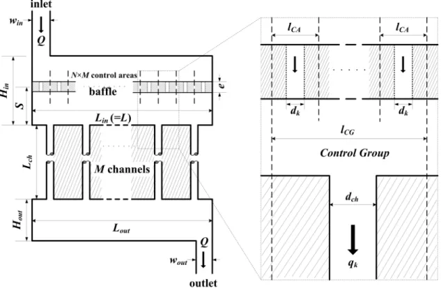
Figure 1 shows a representative schematic view of a multi-tubular equipment to tackle the problem of 1
target flow distribution among parallel channels. The 2D fluid domain consists of 3 sections: inlet 2
distributor, parallel channel array, and outlet collector. The inlet distributor has a single inlet tube of width 3
win, and a distributing manifold of Lin in length and Hin in height. Connected to the distributing manifold are
4
M parallel straight channels of identical width dch and length Lch, evenly spaced between the axis of one
5
channel and another. For convenience of description, they are indexed by k from 1 to M from left to right. 6
The endpoints of parallel channels are connected to the collector, which comprises of a collecting manifold 7
of Lout in length and Hout in height, and a single outlet tube of width wout. Note that the location of the inlet
8
tube (or outlet tube) with respect to the distributing (or collecting) manifold can be on the edge (Fig. 4b), in 9
the middle (Fig. 4a) or at any arbitrary position. 10
11
Fig. 1. Representative 2D schematic view of a multi-tubular equipment with insertion of a perforated baffle. 12
13
A perforated baffle with thickness e is put forward to be installed inside the distributing manifold. The 14
length of the baffle (L) equals to the length of the distributing manifold (Lin), and the distance S between
15
the perforated baffle and the inlets of parallel channels is an adjustable parameter subject to optimization 16
(Luo et al., 2015b). The baffle is divided into M virtual control groups of identical length (lCG), also indexed
17
by k from 1 to M, each control group corresponding to a channel. As a result, the length of control group 18
equals to the pitch between two channels. 19
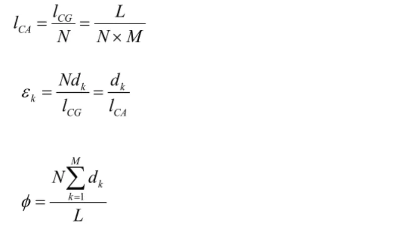
M L
lCG = (1)
20
In kth control group, there exists a number (N) of virtual control areas of identical length (lCA). Each control
21
area has one orifice of width dk arranged in the middle. Then following geometric relations can be easily
22 obtained: 23 M N L N l l CG CA = = × (2) 24 k k k CG CA Nd d l l
ε
= = (3) 25 1 M k kN d
L
φ
=
∑
= (4) 26where εk is defined as the local porosity in the kth control group, which is equal to the local porosity in each
27
control area of the kth control group, Φ the global porosity of the baffle. 28
When a certain fluid with constant mass flow-rate of Q is supplied to the inlet tube, it will subsequently 29
pass through the orifices of the baffle, the parallel channels and finally reach the outlet tube. We annotate 30
the flow-rate passing through the kth channel as qk and its target value as q’k. Based on mass conservation,
31
we obtain: 32
∑
∑
= = = = M k k M k k q q Q 1 ' 1 (5) 1 M Q q = (6) 2where
q
is the mean mass flow-rate of all parallel channels. 32.2. Basic principles 4
To realize the target flow distribution, the evolutionary algorithm is designed to adjust the size distribution 5
of perforated orifices so that the mass flow-rate in each parallel channel approaches its target value. As 6
explained in Fig. 2, the width of orifices in kth control group dk is varied simultaneously by comparing the
7
actual flow-rate qk and its target value q’k in the kth channel. More precisely, if qk is higher than q’k, the size
8
of the orifices dk becomes smaller to reduce the flow-rate passing through the kth channel. Otherwise, if qk
9
is lower than q’k, dk should become larger to increase the downstream fluid flux. According to the repetitive
10
nature of the variation process, an automatic iteration program is developed to realize the iterative 11
procedure until the objective is achieved. 12
13
Fig. 2. Basic principles of the evolutionary algorithm. 14
15
In this study, we follow the variation rule as presented in Eq. (7) from t to t+1 iteration, which introduces a 16
proportional relationship between the variation of dk and the departure of qk from its target q’k.
17 , , , , 1 , k t k t k t k t k t
q
q
d
d
d
q
γ
+′ −
∆
=
−
=
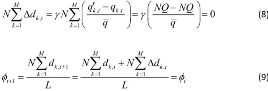
(7) 18γ is a relaxation factor introduced to control the speed of variation. Following this variation rule, it can be 19
observed that although the local porosity εk changes from one iteration to the next, the global porosity of
20
the baffle Φ is kept constant. 21 , , , 1 1
0
M M k t k t k t k kq
q
NQ NQ
N
d
N
q
q
γ
γ
= =′ −
−
∆
=
=
=
∑
∑
(8) 22 , +1 , , 1 1 1 1 M M M k t k t k t k k k t tN d
N d
N
d
L
L
φ
= = =φ
++
∆
=
∑
=
∑
∑
=
(9) 23To avoid the potential possibility of overlap among the orifices, we assume that the boundary of control 24
area and control group is fixed and the size of perforated orifices cannot overstep the boundary of control 25
area during iterations. This implies: 26 1 k k CA d l
ε
= ≤ (10) 272.3. Numerical implementation 1
The evolutionary procedure is described in detail using the flow chart shown in Fig. 3. 2
(1) Input the initial data such as the size and initial geometry of multi-tubular equipment, the 3
general operational conditions (the ambient temperature, operational pressure, with or 4
without heat transfer, etc.), the physical characteristics of working fluid (fluid nature, total inlet 5
flow-rate, density, viscosity, etc.) and the target flow distribution curve. 6
(2) Definition of the parameters relative to the perforated baffle, such as the location and 7
thickness of baffle, the parameter N and the global porosity of the baffle. 8
(3) Mesh generation of the whole simulation domain. Structured mesh is preferable for easy 9
modification of simulation domain boundary. 10
(4) Calculation of the exact flow field at steady state, by solving the Navier-Stokes equations. 11
(5) Calculation of the mass flow-rate qk passing through each parallel channel; modification of the
12
baffle configuration by comparing qk to q’k, according to the variation rule presented in Eq. (7).
13
(6) Regeneration of the mesh for updated simulation domain; recalculation of the exact flow field. 14
(7) Check the stable tolerance of the algorithm. If the tolerance is satisfied, then the evolutionary 15
procedure is terminated. If not so, the procedure goes back to Step 3 for recurrence. The result 16
is considered to be stable when the size variation at t step Δdk,t is smaller than one cell size of
17
the mesh. This also implies that the values of qk and q’k are very close.
18
(8) Exportation of results, including the final configuration of perforated baffle, the values of mass 19
flow-rate in every channel and the total pressure drop. 20
The degree of closeness between the target curve and the final flow distribution curve obtained by 21
performing the evolutionary algorithm is quantified by the deviation factor (DF) defined as follow: 22 2 1
1
DF
1
M k k k kq q
M
=q
−
′
=
′
−
∑
(11) 23The two curves qk and q’k coincide completely when values of DF approach 0. Note that Eq. (11) for flow
24
deviation factor is a generalized form of flow maldistribution factor widely used to indicate the degree of 25
non-uniformity in which
q
is replaced by q’k. Meanwhile, a dimensionless flow-rate ratio is also26
introduced for each channel: 27 D k k q q q q − = (12) 28 29
Fig. 3. Flow chart of the algorithm. 30
31
2.4. Calculation of flow field by CFD method 32
An essential step of the evolutionary algorithm is the calculation of exact flow field. This generally involves 1
solving Navier-Stokes equations by CFD methods. The equation for conservation of mass or continuity 2 equation is: 3 ( ) 0u t
ρ
ρ
∂ + ∇ ⋅ = ∂ (13) 4The momentum conservation equation is described by: 5
( )
u(
uu)
p( )
g F tρ
ρ
ρ
∂ + ∇ ⋅ = −∇ + ∇ ⋅ ∏ + + ∂ (14) 6Where u is the velocity, p is the static pressure,
ρ
g and F are the gravitational body force and 7external body forces,
∏
is the stress tensor which is given by: 8(
T)
2 3 u u uIµ
∏ = ∇ + ∇ − ∇ ⋅ (15) 9where μ is the molecular viscosity, I is the unit tensor. 10
The energy equation is: 11
( )
E(
u E p(
)
)
(
T)
: u QH tρ
ρ
λ
ρ
∂ + ∇ ⋅ + = ∇ ⋅ ∇ + ∏ ∇ + ∂ (16) 12where E is the internal energy,
λ
is the thermal conductivity, and QH includes the heat of chemical13
reaction, radiation and any other volumetric heat sources. 14
To predict turbulent flow pattern, additional turbulence models should be employed. It should be noted 15
that the proposed evolutionary algorithm is somewhat independent of the CFD code used for the 16
calculation of flow fields, regardless whether it is based on finite volume method, finite element method or 17
more advanced techniques such as lattice Boltzmann method (Wang et al., 2010, 2014). 18
Having presented the basic principles and the procedure of the CFD-based evolutionary algorithm, its 19
effectiveness on the realization of target flow distribution will be tested with different geometries of 20
equipment and different target curves. It should be noted that numerical tests carried out in this study did 21
not consider the thermal effect but concentrated on fluid flow. However, the algorithm developed is 22
suitable for conditions with heat transfer, by taking into account the thermal effect in the CFD calculation. 23
24
3. Simulation and results
25
In this section, the simulation and results of several 2D cases are presented to show the feasibility of the 26
proposed evolutionary algorithm. Two geometries of multi-tubular equipment are studied: one symmetric 27
case with middle inlet and outlet (Fig. 4a); another asymmetric case with diagonal inlet and outlet (Fig. 4b). 28
Various target curves are tested, including flat curve, ascending curve, descending curve and step-like 29
curve. 30
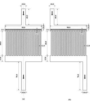
Figure 4 shows the geometry and detail dimensions of studied multi-tubular equipment. The width of the 31
inlet and outlet tube is 10 mm. The length (Lin) of the distributing manifold is 90 mm and the height (Hin) is
15 mm. Identical dimensions are used for the collecting manifold (Lout=90 mm; Hout=15 mm). There are
1
fifteen parallel straight channels (M=15) with identical width (wch) of 2 mm and length (lch) of 60 mm. Note
2
that the unique difference between two tested geometries is the position of inlet and outlet tubes, i.e. in 3
the middle as axisymmetrical geometry (Fig. 4a) or in diagonal as nonaxisymmetrical geometry (Fig. 4b). 4
5
Fig. 4. Geometry and dimensions of studied multi-tubular equipment (unit: mm). (a) middle inlet-outlet; (b) diagonal inlet-outlet. 6
7
The thickness (e) of the perforated baffle is 3 mm and the distance (S) between the baffle and the inlet of 8
parallel channels is 3.5 mm. The baffle is divided into 30 control areas (N=2), the length (lCA) of each control
9
area thus being 3 mm. The initial sizes of orifices are proposed as identical and equal to 1 mm, the global 10
porosity (Φ) being 33%. Recall that according to Eq. (9), the global porosity (Φ) of the baffle is kept constant 11
during iterations. 12
The working fluid used is water with density of 998.2 kg∙m-3 and viscosity of 1.003×10⁻³ kg∙m-1∙s-1. The inlet
13
velocity of fluid is set to be 0.1 m∙s-1, the corresponding Re number being 1000. The Re numbers in parallel
14
straight channels range between 40 and 120. The operational pressure is fixed at 101325 Pa. In this study, 15
simulations are performed under steady state, incompressible and isothermal condition without heat 16
transfer. For simplification, gravity effect is neglected. 17
Fluid flow field in the fluid domain is calculated using a commercial code FLUENT (version 12.1.4). The fluid 18
flow is calculated by the COUPLED method for pressure-velocity coupling, and second-order upwind 19
differential scheme is applied for discretization of momentum and standard method for pressure. Constant 20
velocity normal to the boundary of inlet surface is given and the boundary condition of outlet is set as 21
pressure-outlet with zero static pressure. Adiabatic wall condition is applied and no slip occurs at the wall. 22
The solution is considered to be converged when 1) sums of the normalized residuals for control equations 23
are all less than 1×10⁻⁶and 2) the mass flow-rate at each channel is constant from one iteration to the next
24
(less than 0.5% variation). 25
Structured mesh is generated using software ICEM (version 12.1) to build up the geometry model. 26
Generally, one millimeter is divided into 20 segments to create square elemental cells. The influence of 27
mesh density on the effectiveness of the evolutionary algorithm will be shown in later subsection with 28
numerical example. At each optimization step, MATLAB is used to take the computed flow field results from 29
FLUENT, perform calculations of the coordinates of simulation domain and pass the data required to ICEM 30
to regenerate the mesh for the updated geometry. 31
3.1. Middle inlet-outlet geometry 32
Two target curves will be tested for the middle inlet-outlet geometry. The first is a flat curve implying 33
uniform flow distribution while the second one is an ascending curve representing non-uniform flow 34
distribution. These target curves can be described by the formulas below: 35
(
1,2,...,15)
′ = = = k Q q q k M (17) 36(
)
2(
)
1
196
1,2,...,15
3955
−
+
′ =
=
kk
q
Q
k
(18) 373.1.1. Flat target curve
1
Figure 5 shows the flow-rate ratio of each channel under different conditions. When no baffle is stalled in 2
the distributing manifold, the fluid tends to go preferentially into the channels facing the inlet tube. The 3
flow distribution among parallel channels is obviously not uniform (maximum value of Dqk is 58%). The flow
4
distribution is symmetrical about the central 8th channel due to the axisymmetry of the geometry. The
5
insertion of a uniformly perforated baffle (initial baffle) serves as an additional flow resistance to improve 6
the uniformity to some extent, but still way off the target curve (maximum value of Dqk is 23%). By running
7
the proposed evolutionary algorithm to adjust the sizes of orifices, uniform flow distribution among parallel 8
channels can be achieved as shown by contour of velocity magnitude in Fig. 6, indicated by the almost flat 9
optimized distribution curve (maximum value of Dqk is -1.4%).
10
Figure 7 shows the evolution of DF values and the total pressure drop as a function of optimization steps. 11
The step -1 represents the empty distributing manifold without baffle and the step 0 stands for the initial 12
configuration of the baffle with identical size of orifices (same notations hereafter). It can be observed that 13
the DF value reduces from 0.209 to 0.009 after 3 optimization steps, while the total pressure drop increases 14
from 21.2 Pa to 24.0 Pa. This case study implies that the proposed evolutionary algorithm is efficient for 15
fluid flow homogenization. More details on the performance of evolutionary algorithm for uniform flow 16
distribution, especially the effects of the baffle location, the initial size distribution of orifices and the global 17
porosity can be found in our earlier work (Luo et al., 2015b). 18
19
Fig. 5. Flow distribution among parallel channels (middle inlet-outlet geometry; flat target curve). 20
21
Fig. 6. Contours of velocity magnitude (middle inlet-outlet geometry; flat target curve). 22
23
Fig. 7. Deviation factor (DF) and pressure drop (Δp) as a function of optimization step (middle inlet-outlet geometry; flat target 24
curve). 25
26
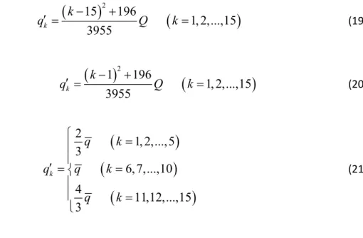
3.1.2. Ascending target curve
27
An ascending target curve is also introduced to test the objective of non-uniform flow distribution, and the 28
optimization results are shown in Fig. 8. Unlike the flat target curve case, the flow flux in channels 1-9 29
should be reduced while those in channels 10-15 should be raised to approach the target values. This raises 30
a higher requirement to the optimization algorithm because a simple action of homogenization is not 31
sufficient. It can be observed from Fig. 8 that using the proposed evolutionary algorithm, the ascending 32
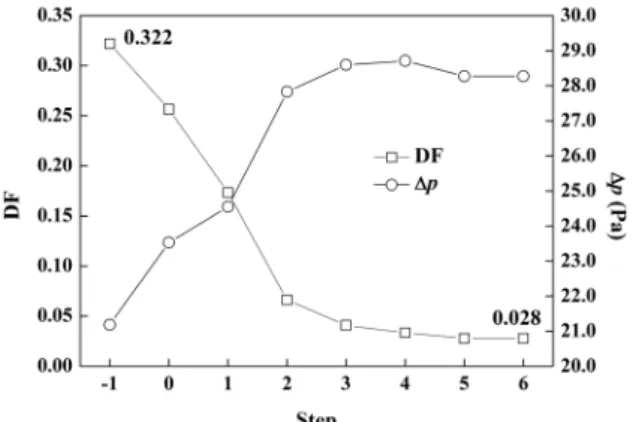
target curve can be largely approached. The value of DF reduces from 0.322 to 0.028 after 6 optimization 33
steps while the total pressure drop increases from 21.19 Pa to 28.27 Pa, as shown in Fig. 9. Compared to 34
the flat target curve case, the optimization procedure is a bit longer and higher pressure drop is generated. 35
However, 33% increase in pressure drop is generally acceptable compared to the 91.3% reduction in DF. 36
This case study indicates that the proposed CFD-based evolutionary algorithm is capable of realizing target 37
asymmetrical flow distribution for an axisymmetrical geometry. 38
39
Fig. 8. Flow distribution among parallel channels (middle inlet-outlet geometry; ascending target curve). 40
1
Fig. 9. Deviation factor (DF) and pressure drop (Δp) as a function of optimization step (middle inlet-outlet geometry; ascending 2
target curve). 3
4
3.2. Diagonal inlet-outlet geometry 5
Three patterns of target curve are tested for the diagonal inlet-outlet geometry, including a descending 6
curve, an ascending curve and a step-like curve. These target curves can be described by the formulas 7 below: 8
(
)
2(
)
15
196
1,2,...,15
3955
−
+
′ =
=
kk
q
Q
k
(19) 9(
)
2(
)
1
196
1,2,...,15
3955
−
+
′ =
=
kk
q
Q
k
(20) 10(
)
(
)
(
)
2 1,2,...,5 3 6,7,...,10 4 11,12,...,15 3 = ′ = = = k q k q q k q k (21) 113.2.1. Descending target curve
12
Unlike the middle inlet-outlet case, the initial flow distribution curve of the diagonal inlet-outlet geometry 13
(without baffle) is nonaxisymmetric and irregular, due to the inherent nonaxisymmetry of the geometry 14
tested. As shown in Fig. 10, the flow-rate achieves the highest value in channel 2 and then decreases 15
rapidly to the lowest in channel 5. After that, a monotonous increase of flow-rate appears till the channel 16
15 which is the farthest channel from the inlet tube. The insertion of perforated baffle of uniform-sized 17
orifices would improve the distribution uniformity, but does not much alter the global shape of the 18
distribution curve. It seems that the uniform perforated baffle is not efficient to achieve non-uniform flow 19
distribution in a nonaxisymmetrical structure. By performing the proposed evolutionary algorithm however, 20
a good agreement can be reached between the optimized distribution curve and the target. 21
22
Fig. 10. Flow distribution among parallel channels (diagonal inlet-outlet geometry; descending target curve). 23
24
As shown in Fig. 11, the value of DF is reduced by 95.1% from 0.350 to 0.017 in 8 optimization steps, at the 25
cost of 29.8% increase in pressure drop (from 25.58 Pa to 33.20 Pa). In fact, higher pressure drop is 26
generally inevitable to change the normal distribution to a target curve. The evolutionary algorithm may 27
propose an optimal structure with balanced energy cost and the achievement of distribution target. 28
Fig. 11. Deviation factor (DF) and pressure drop (Δp) as a function of optimization step (diagonal inlet-outlet geometry; descending 1
target curve). 2
3
3.2.2. Ascending target curve
4
Right now, an ascending curve is considered to be the target. The flow distribution curves for initial shape 5
(without baffle) and for uniform perforated baffle are the same as described for the descending target 6
curve case. By comparing the initial distribution curve and the target curve (Fig. 12), it can be observed that 7
great reduction in flow-rate is required for channels 1-3 facing the inlet tube while the fluxes in other 8
channels are relatively closer to their target values. 9
10
Fig. 12. Flow distribution among parallel channels (diagonal inlet-outlet geometry; ascending target curve). 11
12
It can also be observed from Fig. 12 that the optimized distribution curve and the target curve are largely 13
matched while noticeable discrepancy may be found for channels 1-2. This is mainly due to the mesh 14
density, i.e. the minimum amount of geometry change is one mesh cell. In this study, one millimeter is 15
divided into 20 segments (0.05 mm for a cell) for a compromise between accuracy and computational time. 16
With this density, the value of DF decreases from 0.331 to about 0.028 in 7 steps but can not be reduced 17
further, as shown in the left part of Fig. 13. Higher mesh density is favorable for a subtle modification of 18
baffle geometry thus has positive effect on the realization of target flow distribution. As shown in the right 19
part of Fig. 13, the value of DF could be further reduced from 0.028 to 0.018 in three steps when the size of 20
single cell is decreased from 0.05 mm to 0.02 mm. Nevertheless, higher mesh density augments the 21
computational burden and raises higher requirement on the precision of fabrication method. 22
23
Fig. 13. Deviation factor (DF) and pressure drop (Δp) as a function of optimization step, influence of mesh density (diagonal 24
inlet-outlet geometry; descending target curve). 25
26
3.2.3. Step-like target curve
27
The two target curves studied above are both gradual, and this time a step-like target curve is introduced to 28
test the effectiveness of the proposed algorithm. The step-like curve is mathematically described in Eq. (21). 29
Graphically, 15 parallel channels are classified into low flow-rate group (channels 1-5), middle flow-rate 30
group (channels 6-10) and high flow-rate group (channels 11-15). Uniform flow distribution is required 31
among channels of the same group but the ratio of high and low flux is 2. 32
33
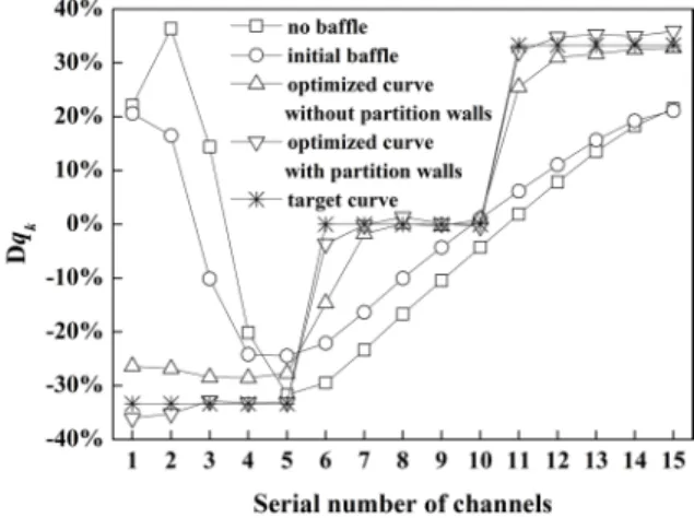
Fig. 14. Flow distribution among parallel channels, effect of partition walls (diagonal inlet-outlet geometry; step-like target curve). 34
35
By examining the optimized curve (shown by marker ∆) in Fig. 14, it can be observed that the step-like 36
target curve (shown by marker *) can be satisfied only in tendency. The fluid fluxes in channels 6 and 11 37
can not rise to their target values while those in channels 1-5 are higher than the set value. This is because 38
when a flow-rate jump is required from one channel to its neighbor, i.e. from channel 5 (10) to channel 6 1
(11), high velocity gradient exists so that a transversal flow flux is inevitable at the remixing area between 2
the perforated baffle and the channel inlets. As a result, the flow-rate in the first channel of step (channel 6 3
and channel 11) is difficult to reach its target value. 4
If a more satisfying optimized distribution curve is expected, a practical solution that can be easily 5
employed is adding partition walls between the baffle and the channel inlets, to avoid the transitional flow 6
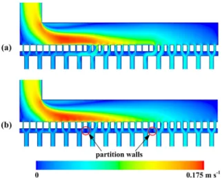
flux. A comparative test is then carried out. As shown in Fig. 15b, two partition walls are installed in the 7
middle of channels 5 and 6, and of channels 10 and 11, respectively. Other numerical parameters are kept 8
unchanged. In this situation, the optimization objective is to realize uniform flow distribution in three 9
separated groups isolated from each other. The optimized curve of the improved method (shown by 10
marker ∇) is also shown in Fig. 14. It can be observed that the optimized flow fluxes in channels 6 and 11 11
are closer to their target values, implying a good accordance between the optimized curve and the target 12
curve. 13
14
Fig. 15. The effect of parathion walls on the flow field. (a) without partition walls; (b) with partition walls. 15
16
The effect of partition walls on the controlled flow distribution is shown in Fig. 16. It can be observed that 17
the value DF can be further reduced from 0.052 to 0.019 by adding partition walls with a negligible increase 18
in total pressure drop. This case study indicates that when target flow-rate gradient is important between 19
two neighboring channels, adding partition walls to avoid the transitional flux is an effective solution, as 20
shown in Fig. 15. 21
22
Fig. 16. Deviation factor (DF) and pressure drop (Δp) as a function of optimization step, effect of partition walls (diagonal 23
inlet-outlet geometry; step-like target curve). 24
25
3.3. The configurations of the optimized perforated baffle 26
Figure 17 shows the dimension distribution of orifices on the optimized perforated baffle subject to 27
different target curves. A dimensionless diameter ratio (Ddk) is introduced for each orifice for comparison:
28
D
k kd
d
d
d
−
=
(22) 29where d is the average diameter of all orifices. 30
31
Fig. 17. Optimal dimensions of orifices for different target curves. (a) middle inlet-outlet geometry; (b) diagonal inlet-outlet 32
geometry. 33
Obviously, the optimal dimensions of orifices are very different from one case to another. For each case, it 1
can be observed that the dimension distribution of orifices is roughly related to the difference between the 2
initial distribution curve and the target distribution curve. This is logic since it is the basic principle of the 3
evolutionary algorithm for optimization. However, quantitative relationships seem difficult to be obtained 4
at this stage because of various interactions of fluid flows before and after they passing through the orifices, 5
especially for cases of non-uniform target curves. 6
7
4. Discussion and conclusions
8
A CFD-based evolutionary algorithm is proposed for the realization of target flow distribution among 9
parallel channels. The algorithm adjusts the size of orifices on the perforated baffle inserted in the 10
distributing manifold so as to approach the target flow flux in every parallel channel. The effectiveness of 11
the proposed evolutionary algorithm is tested by several 2D examples with different geometries 12
(axisymmetric or nonaxisymmetric) and different target curves (uniform or non-uniform). Results show that 13
for most of the cases, the optimized distribution curve rapidly reached by the algorithm is in good 14
agreement with the target curve. The application of the algorithm is rather wide and promising. It can 15
provide simple and practical solution for various engineering fields dealing with fluid distribution problem. 16
The influence of mesh density on the optimization results is analyzed through one special case. Generally, 17
refined mesh (higher density) is favorable for more accurate calculation and more subtle modification of 18
the baffle geometry. However, it raises higher requirements on computational facilities and the fabrication 19
precision. Progressively refinement technique may be used to save the computation time. For practical 20
applications of the algorithm in real engineering, the smallest cell size could be determined considering the 21
fabrication precisions and tolerable deviation from the target curve. 22
The case study of “step-like” target curve shows that adding partition walls is effective to eliminate the 23
transversal flux due to high flow-rate gradient between neighboring parallel channels. Hence this action can 24
be considered as a useful complementary to the proposed algorithm. Under extreme operating conditions, 25
partition walls may be installed for every “control group”. The orifices in each control group functions as a 26
“static valve” to adjust the desired flow-rate in the corresponding straight channel. 27
The perforated baffle may also be installed in the collecting manifold as additional resistance to adjust the 28
fluid flow distribution. However, a preliminary test shows that the downstream control may not be as 29
efficient as upstream control so it is not recommended. An alterative solution is to adjust the dimension of 30
the inlet/outlet opening of every parallel channel as a supplemental hydraulic resistance. The optimized 31
distribution of openings plays the role of integrated perforated baffle, leading to the target flow 32
distribution among parallel channels. A systematic study on this method is one of the directions of our 33
future work. 34
It should be noted that the efficiency of the proposed algorithm depends largely on simulated flow field 35
while there is always a departure from the reality. Experimental validation of the proposed algorithm is also 36
our ongoing work. This concerns the simulation and optimization of 3D objects, their fabrication and 37
characterization. The extension of the heuristic algorithm for 3D applications is in principle straightforward 38
and some guidelines can be found in Ref. (Luo et al., 2015b). 39
Finally, we shall return to the notion of “flow maldistribution”. Flow maldistibution is usually considered as 40
equivalent to non-uniform (uneven, inhomogeneous, etc.) flow distribution, meaning the common 41
phenomenon of flow-rate difference among the different channels of multi-tubular equipment. The 42
implication of this term is that any deviation from the uniform is considered as bad (mal)distribution. Under 1
real operating conditions however, the optimal flow distribution is usually not uniform but obeys certain 2
trend subject to a defined optimization objective and constraints. As a result, the notion of “flow 3
maldistribution” should be addressed in a broader context than uneven flow distribution: any flow
4
distribution that differs from the optimal distribution is referred as maldistribution. According to this new 5
definition, the parameter that indicates the departure between a certain distribution and its optimal shape, 6
i.e. the factor DF defined in Eq. (11), should be named as the general “maldistribution factor (MF)”. 7
The proposed evolutionary algorithm for the realization of target distribution is just a small step to tackle 8
the flow maldistribution problem within its general framework. But behind all these, the deeper question is 9
“what kind of flow distribution is the optimal”? This involves the determination of the “target curve” for a 10
process device or system, based on the defined objective function and constraints. This is also our on-going 11 work. 12 13 Acknowledgement 14
This work is partially financed by the French CNRS within the project AAP-Energie 2012 of INSIS. One of the 15
authors M. Min WEI would like to thank the “Région Pays de la Loire” for its partial financial support to his 16
PhD study. 17
Notations
1
d average diameter of all orifices m
dch diameter of parallel channels m
dk diameter of orifices m
Ddk dimensionless diameter ratio -
DF deviation factor -
Dqk dimensionless flow-rate ratio -
e thickness of the perforated baffle m
E internal energy per unit mass J kg-1
F external body force kg m s-2
g gravitational acceleration m s-2
Hin length of distributing manifold m
Hout length of collecting manifold m
I unit tensor -
lCA length of control area m
lCG length of control group m
L length of baffle m
Lch length of parallel channels m
Lin length of inlet tube m
Lout length of outlet tube m
M number of parallel channels -
N number of control areas in each control group -
p pressure Pa
q
mean mass flow-rate among parallel channels kg s-1k
q mass flow-rate through channel k kg s-1
k
q′ objective mass flow-rate through channel k kg s-1
Q total inlet mass flow-rate kg s-1
QH external heat transfer flux J kg-1 s-1
S distance between baffle and parallel channels m
t time step -
T temperature K
u velocity m s-1
win width of inlet tube m
wout width of outlet tube m
Greek symbols 2
γ
relaxation factor - ε local porosity -λ
thermal conductivity W m-1 K-1 µ viscosity kg m-1 s-1∏
stress tensor - ρ density kg m-3 Φ global porosity - Subscriptsk channel and orifice index
References
1
Al-Rawashdeh, M., Yu, F., Patil, N.G., Nijhuis, T.A., Hessel, V., Schouten, J.C., Rebrov, E.V., 2014. 2
Designing flow and temperature uniformities in parallel microchannels reactor. AIChE Journal 60(5), 3
1941-1952. 4
Boerema, N., Morrison, G., Taylor, R., Rosengarten, G., 2013. High temperature solar thermal 5
central-receiver billboard design. Solar Energy, 97, 356-368. 6
Chiou, J.P., 1978. Thermal performance deterioration in crossflow heat exchanger due to the flow 7
nonuniformity. ASME Journal of Heat Transfer, 100, 580-587. 8
Chiou, J.P., 1982. The effect of nonuniform fluid flow distribution on the thermal performance of solar 9
collector. Solar Energy, 29(6), 487-502. 10
Commenge, J., Falk, L., Corriou, J., Matlosz, M., 2002. Optimal design for flow uniformity in microchannel 11
reactors. AIChE Journal, 48(2), 345-358. 12
Fan, Y., Boichot, R., Goldin, T., Luo, L., 2008. Flow distribution property of the constructal distributor and 13
heat transfer intensification in a mini heat exchanger. AIChE Journal, 54(11), 2796-2808. 14
Fleming, R.B., 1967. The effect of flow distribution in parallel channels of counter-flow heat exchangers. 15
Advances in Cryogenic Engineering, 12, 352-362. 16
Guo, X., Fan, Y., Luo, L., 2014. Multi-channel heat exchanger-reactor using arborescent distributors: A 17
characterization study of fluid distribution, heat exchange performance and exothermic reaction. Energy, 69, 18
728-741. 19
Heibel, A.K., Scheenen, T.W.J., Heiszwolf, J.J., Van As, H., Kapteijn, F., Moulijn, J.A., 2001. Gas and liquid 20
phase distribution and their effect on reactor performance in the monolith film flow reactor. Chemical 21
Engineering Science, 56(21-22), 5935-5944. 22
Inoue, T., Schmidt, M.A., Jensen, K.F., 2007. Microfabricated Multiphase Reactors for the Direct Synthesis 23
of Hydrogen Peroxide from Hydrogen and Oxygen. Industrial and Engineering Chemistry Research, 46(4), 24
1153-1160. 25
Jiao, A., Zhang, R., Jeong, S.K., 2003. Experimental investigation of header configuration on flow 26
maldistribution in plate-fin heat exchanger. Applied thermal engineering, 23(10), 1235-1246. 27
Jones, G.F., 1987. Consideration of the heat-removal factor for liquid-cooled flat-plate solar collectors. Solar 28
Energy, 38(6), 455-458. 29
Kobayashi, J., Mori, Y., Okamoto, K., Akiyama, R., Ueno, M., Kitamori, T., Kobayashi, S., 2004. A 30
Microfluidic Device for Conducting Gas-Liquid-Solid Hydrogenation Reactions. Science, 304, 1305-1308. 31
Kumaran, R.M., Kumaraguruparan, G., Sornakumar, T., 2013. Experimental and numerical studies of 1
header design and inlet/outlet configurations on flow mal-distribution in parallel micro-channels. Applied 2
Thermal Engineering, 58, 205-216. 3
Lalot, S., Florent, P., Lang, S., Bergles, A., 1999. Flow maldistribution in heat exchangers. Applied thermal 4
engineering, 19(8), 847-863. 5
Luo, L., 2013. Heat and Mass Transfer Intensification and Shape Optimization: A Multi-scale Approach. 6
Springer, London. 7
Luo, L., Fan, Y., Wei, M., Flamant, G., 2015a. Method for determing characteristics of holes to be provided 8
through a plate and corresponding programme. WO 2015/028758. 9
Luo, L., Fan, Y., Zhang, W., Yuan, X., Midoux, N., 2007. Integration of constructal distributors to a mini 10
crossflow heat exchanger and their assembly configuration optimization. Chemical engineering science, 11
62(13), 3605-3619. 12
Luo, L., Wei, M., Fan, Y., Flamant, G., 2015b. Heuristic shape optimization of baffled fluid distributor for 13
uniform flow distribution. Chemical Engineering Science, 123, 542-556. 14
Maharaj, L., Pocock, J., Loveday, B., 2007. The effect of distributor configuration on the hydrodynamics of 15
the teetered bed separator. Minerals Engineering, 20(11), 1089-1098. 16
Milman, O.O., Spalding, D.B., Fedorov, V.A., 2012. Steam condensation in parallel channels with 17
nonuniform heat removal in different zones of heat-exchange surface. International Journal of Heat and 18
Mass Transfer, 55, 6054-6059. 19
Ong, B., Gupta, P., Youssef, A., Al-Dahhan, M., Dudukovic, M., 2009. Computed tomographic investigation 20
of the influence of gas sparger design on gas holdup distribution in a bubble column. Industrial & Engineering 21
Chemistry Research, 48(1), 58-68. 22
Ponzi, P.R., Kaye, L.A., 1979. Effect of flow maldistribution on conversion and selectivity in radial flow 23
fixed-bed reactors. AIChE Journal, 25(1), 100-108. 24
Rebrov, E.V., Ismagilov, I.Z., Ekatpure, R.P., de Croon, M.H.J.M., Schouten, J.C., 2007. Header design for 25
flow equalization in microstructured reactors. AIChE Journal, 53(1), 28-38 26
Rebrov, E.V., Schouten, J.C., De Croon, M.H.J.M., 2011. Single-phase fluid flow distribution and heat 27
transfer in microstructured reactors. Chemical Engineering Science, 66(7), 1374-1393. 28
Saber, M., Commenge, J.-M., Falk, L., 2010. Microreactor numbering-up in multi-scale networks for 29
industrial-scale applications: Impact of flow maldistribution on the reactor performance. Chemical 30
Engineering Science, 65(1), 372-379. 31
Tondeur, D., Fan, Y., Commenge, J.-M., Luo, L., 2011. Uniform flows in rectangular lattice networks. 1
Chemical Engineering Science, 66(21), 5301-5312. 2
Wada, Y., Schmidt, M.A., Jensen, K.F., 2006. Flow distribution and ozonolysis in gas−liquid multichannel 3
microreactors. Industrial and Engineering Chemistry Research, 45(24), 8036-8042. 4
Wang, L., Fan, Y., Luo, L., 2010. Heuristic optimality criterion algorithm for shape design of fluid flow. 5
Journal of Computational Physics, 229(20), 8031-8044. 6
Wang, L., Fan, Y., Luo, L. 2014. Lattice Boltzmann method for shape optimization of fluid distributor. 7
Computers & Fluids, 94(1), 49-57. 8
Wang, X., Wu, L., 1990. Analysis and performance of flat-plate solar collector arrays. Solar Energy, 45(2), 9
71-78. 10
Wen, J., Li, Y., 2004. Study of flow distribution and its improvement on the header of plate-fin heat 11
exchanger. Cryogenics, 44(11), 823-831. 12
Yue, J., Boichot, R., Luo, L., Gonthier, Y., Chen, G., Yuan, Q., 2010. Flow distribution and mass transfer in 13
a parallel microchannel contactor integrated with constructal distributors. AIChE Journal, 56(2), 298-317. 14
List of figures
1
2
Figure 1. Representative 2D schematic view of a multi-tubular equipment with insertion of a perforated baffle.
3
(a)
(b)
1
Figure 2. Basic principles of the algorithm.
2
3
Figure 3. Flow chart of the algorithm.
1
Figure 4. Geometry and dimensions of studied multi-tubular equipment (unit: mm): (a) middle inlet-outlet; (b)
2
diagonal inlet-outlet.
3
4
Figure 5. Flow distribution among parallel channels (middle inlet-outlet geometry; flat target curve).
1
Figure 6. Contours of velocity magnitude (middle inlet-outlet geometry; flat target curve).
2
3
Figure 7. Deviation factor (DF) and pressure drop (Δp) as a function of optimization step (middle inlet-outlet
4
geometry; flat target curve).
5
1
Figure 9. Deviation factor (DF) and pressure drop (Δp) as a function of optimization step (middle inlet-outlet
2
geometry; ascending target curve).
3
4
Figure 10. Flow distribution among parallel channels (diagonal inlet-outlet geometry; descending target curve).
5
6
Figure 11. Deviation factor (DF) and pressure drop (Δp) as a function of optimization step (diagonal inlet-outlet
7
geometry; descending target curve).
1
Figure 12. Flow distribution among parallel channels (diagonal inlet-outlet geometry; ascending target curve).
2
3
Figure 13. Deviation factor (DF) and pressure drop (Δp) as a function of optimization step, influence of mesh
4
density (diagonal inlet-outlet geometry; descending target curve).
5
6
Figure 14. Flow distribution among parallel channels, effect of partition walls (diagonal inlet-outlet geometry;
7
step-like target curve).
1
Figure 15. The effect of parathion walls on the flow field. (a) without partition walls; (b) with partition walls.
2
3
Figure 16. Deviation factor (DF) and pressure drop (Δp) as a function of optimization step, effect of partition
4
walls (diagonal inlet-outlet geometry; step-like target curve).
5
(a)
(b)
1
Figure 17. Optimal dimensions of orifices for different target curves. (a) middle inlet-outlet geometry; (b)
2
diagonal inlet-outlet geometry.
3 4