Colour-magnitude diagrams of transiting Exoplanets - II.
A larger sample from photometric distances
Amaury H. M. J. Triaud
1,2?, Audrey A. Lanotte
3, Barry Smalley
4and Micha¨
el Gillon
31Kavli Institute for Astrophysics & Space Research, Massachusetts Institute of Technology, Cambridge, MA 02139, USA 2Fellow of the Swiss national science foundation
3Institut d’Astrophysique et de G´eophysique, Universit´e de Li`ege, All´ee du 6 Aoˆut 17, Sart Tilman, 4000 Li`ege 1, Belgium 4Astrophysics Group, Keele University, Staffordshire, ST5 5BG, UK
Accepted ?. Received ?; in original form ?
ABSTRACT
Colour-magnitude diagrams form a traditional way of presenting luminous objects in the Universe and compare them to each others. Here, we estimate the photometric distance of 44 transiting exoplanetary systems. Parallaxes for seven systems confirm our methodology. Combining those measurements with fluxes obtained while planets were occulted by their host stars, we compose colour-magnitude diagrams in the near and mid-infrared. When possible, planets are plotted alongside very low-mass stars and field brown dwarfs, who often share similar sizes and equilibrium temperatures. They offer a natural, empirical, comparison sample. We also include directly imaged exoplanets and the expected loci of pure blackbodies.
Irradiated planets do not match blackbodies; their emission spectra are not featureless. For a given luminosity, hot Jupiters’ daysides show a larger variety in colour than brown dwarfs do and display an increasing diversity in colour with decreasing intrinsic luminosity. The presence of an extra absorbent within the 4.5 µm band would reconcile outlying hot Jupiters with ultra-cool dwarfs’ atmospheres. Measuring the emission of gas giants cooler than 1 000 K would disentangle whether planets’ atmospheres behave more similarly to brown dwarfs’ atmospheres than to blackbodies, whether they are akin to the young directly imaged planets, or if irradiated gas giants form their own sequence.
Key words: planetary systems – planets and satellites: atmospheres – binaries: eclips-ing – stars: distances – brown dwarfs – Hertzsprung–Russell and colour–magnitude diagrams.
It is trivial to convert fluxes measured at occultation, or obtained while observing the phase curves of transit-ing exoplanets into absolute magnitudes. One only needs a distance measurement. Two colour-magnitude diagrams for transiting –or occulting– exoplanets were presented in Tri-aud(2014) for seven systems that have Hipparcos parallaxes
(van Leeuwen 2007). Coincidentally, this happened
approxi-mately a century after the first Herzsprung-Russell diagrams were composed (Hertzsprung 1911;Russell 1914a,b,c).
Colour-magnitude diagrams offer a means to compare exoplanets with each others, using natural units for ob-servers. In addition, they allow to infer global properties without requiring the need to fit complex atmospherical models through the sparse data points that can only be gathered at this stage. Those inferences can be made by
? E-mail: triaud@mit.edu
comparing exo-atmospheres to other objects having simi-lar temperatures and sizes; very low-mass stars and field brown dwarfs are a readily available and well-studied sam-ple. Young, directly imaged planets are routinely compared to field brown dwarfs for this very reason (e.g. Bonnefoy
et al. 2013). Finally, irradiated and non-irradiated gas
gi-ants can be compared to each others in colour-magnitude space. Those diagrams can offer a tool to pinpoint the pro-cesses that lead highly irradiated planets to be bloated (e.g.
Demory & Seager 2011).
Just as the construction of the Herzsprung-Russell dia-gram led to vast advances in stellar formation and evolution, the compilation of colour-magnitude diagrams for transiting exoplanets will likely spur similar developments. Models in colour-space may predict that different planet families have distinct locations or sequences (dependent on their gravity, their atmospheric structure, their relative abundances...). This would provide diagnostics to select suitable targets for
(a) χ2r = 0.3 ± 0.4 0 50 100 150 0 50 100 150 −20 −10 0 10 20 Distance (pc), parallaxes
Distance (pc), Torres et al. (2008)
∆ distance . . . . . . . . (b) χ2r= 2.7 ± 0.8 0 50 100 150 0 50 100 150 −20 0 20 Distance (pc), parallaxes
Distance (pc), this paper
∆ distance . . . . (c) χ2r = 1.1 ± 0.4 0 100 200 300 400 500 600 0 100 200 300 400 500 600 −100−50 0 50 100
Distance (pc), this paper
Distance (pc), Torres et al. (2008)
∆ distance . . . .
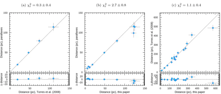
Figure 1. Distance measurements compared with one another, from our sample, including the two discrepant stars GJ 436 and GJ 1214. Reduced χ2
r are given. a) parallactic distances from Hipparcos versus photometric distances fromTorres, Winn & Holman(2008). b) parallactic distances from Hipparcos versus photometric distances estimated in this paper. c) photometric distances fromTorres, Winn
& Holman(2008) versus photometric distances estimated in this paper.
further follow-up, in a fashion similar to selecting a partic-ular stellar population, for instance, to remove giant con-taminants prior to a survey focusing on G and K dwarfs. In the case of irradiated gas giants specifically, the lack of cloud cover may cause objects to fall in a specific region in colour-space. Being identifiable, it will help optimise the de-tection of atmospheric features in transmission. In addition, if planets follow defined sequences, magnitudes obtained in one band lead to accurate predictions for others bands. It can only encourage observations at wavelengths more diffi-cult to obtain.
In total, 44 systems (43 planets and one brown dwarf) have been observed at occultation and were present in the literature. Rather than waiting for GAIA (e.g. Perryman
et al. 2001) to deliver its much awaited parallaxes, this
pa-per will instead use photometric distances. Thanks to their transiting configurations and to the intensive observational efforts that has been undertaken both in the confirmation and in the characterisation of these objects, the fundamental stellar parameters are accurately known. This means that re-liable distances can be computed such as was done for exam-ple byTorres, Winn & Holman(2008). Hertzsprung-Russell diagrams can be represented as luminosity versus effective temperature. We instead opted for using colours instead of temperatures (Beatty et al. 2014), because magnitudes are closer to direct observables.
The paper is organised in the following way: we first out-line our procedure to measure photometric distances (Sec.1) and then describe how the host stars’ apparent magnitudes were determind from the Spitzer photometry (Sec.2). In the following section, different colour-magnitude diagrams are drawn and described in qualitative and quantitative ways. We then discuss our results and conclude.
1 THE DETERMINATION OF PHOTOMETRIC DISTANCES
Our distances are derived from catalogued parameters: we obtained effective temperatures (Teff), surface
grav-ities (log g) and metallicgrav-ities ([Fe/H]) from TEPCAT1
(Southworth 2011) and used those to compute stellar radii
(R?) thanks to a relation provided inTorres, Andersen &
Gim´enez(2010) (Ch. 8). R?and Teff directly lead to
stel-lar luminosities (L?) that were in turn converted into
bolo-metric magnitudes (Mbol) using the following relation (Cox
2000):
Mbol= 4.75 − 2.5 log L? (1)
Absolute visual magnitudes (MV) were estimated thanks to
bolometric corrections estimated by Flower(1996); values are provided in TableB2.
We explored the Tycho2 catalogue (Høg et al. 2000) to compile a list of apparent visual magnitude mV. Failing
to find a number of systems we turned to APASS/UCAC4
(Zacharias et al. 2013) and then to TASS (Droege et al.
2006). Distances were obtained from the distance modulus (mV− MV). Errors are propagated throughout.
No reddening corrections, E(B − V ) were applied since they are not available for most of our sample. We expect most E(B − V ) < 0.1, leading to offsets AV < 0.33 on
(mV− MV) (Maxted, Koen & Smalley 2011).
The distances we calculated are given in TableB2and are visually represented in Figure1. Those plots show our re-sults compared to corresponding distances from the revised Hipparcos catalog (van Leeuwen 2007). We also compare our estimates to photometric distances fromTorres, Winn
& Holman(2008), which provides a wider range and greater
(a) χ2r = 0.7 ± 0.2 4 6 8 10 12 4 6 8 10 12 −0.2 −0.10.0 0.1 0.2 WISE 1 W1 − [3.6] [3.6 µm], this paper . . . . (b) χ2r = 1.7 ± 0.3 4 6 8 10 12 4 6 8 10 12 −0.2 −0.10.0 0.1 0.2 . . . . WISE 2 W2 − [4.5] [4.5 µm], this paper
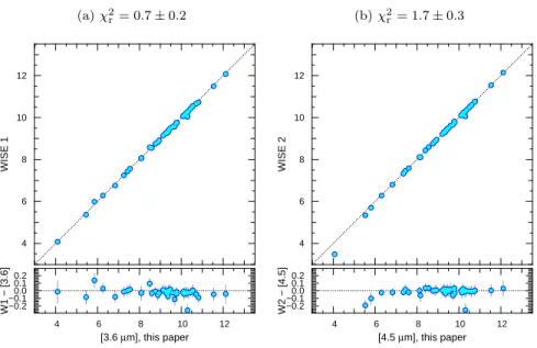
Figure 2. Apparent magnitude measurements comparing those obtained by WISE to those that we estimated, from the Spitzer images. CoRoT-2A is clearly discrepant in both, because it is blended with CoRoT-2B the WISE data. Reduced χ2
r are given. a) on a band centred around 3.6 µm. b) on a band centred around 4.5 µm. The discrepant point at ∼ 10.3 is the CoRoT-2 system. Objects > 6th magnitude appear brighter in the WISE 2 band, which may be due to some detector effects. Discrepant points removed, χ2
r < 1.
overlap of systems than Hipparcos. Our two most discrepant distance measurements are on GJ 436 and GJ 1214. This is most probably caused by the late type of both stars, who, with masses < 0.6 M , fall outside the range over which
the Torres relation has been calibrated for. We thus adopt the most recent distance estimates, fromvan Leeuwen(2007) and fromAnglada-Escud´e et al.(2013) respectively. Remov-ing those two objects, the reduced χ2r for Fig. 1bchanges
from 2.7 ± 0.8 to 0.6 ± 0.4. All comparisons lead to reduced χ2r ∼ 1. Reddening is thus contained within our error bars.
2 THE DETERMINATION OF SPITZER APPARENT MAGNITUDES
The WISE satellite (Cutri & et al. 2012) has two bandpasses, W1 and W2, that resemble two of Spitzer’s IRAC channels.
Kirkpatrick et al. (2011) showed the colour agreement
be-tween both spacecrafts, on field brown dwarfs. Needing to use the IRAC 3 & 4, for which there is no WISE equiva-lent, we derived photometry from all Spitzer channels and compared the [3.6] and [4.5] to W1 and W2, to validate our measurements in the redder channels.
We searched the Spitzer Heritage Archive2for all frames
obtained on the targets with reported occultations in the published literature (TableB4). Apparent magnitudes were obtained for each set of observations. Our methods for ex-tracting the photometry are located in appendixA, and here summarised. We perform aperture photometry on the IRAC images calibrated by the standard Spitzer pipeline accord-ing to the EXOPHOT pyraf pipeline followaccord-ing Lanotte et al. (in prep). Stellar flux is corrected for contribution from visual companions, if relevant. We average those flux and convert
2 http://sha.ipac.caltech.edu/applications/Spitzer/SHA/
them into Vega apparent magnitudes following the methods described byReach et al.(2005). When several observations were made of the same stars, we computed the optimal aver-age of their apparent magnitude in each of Spitzer’s Astro-nomical Observation Request (AOR) to produce the values located in tableB2.
Our estimates are graphically compared in Fig.2to cor-responding bands employed by the WISE satellite. Reduced χ2
r are calculated. They indicate very good agreement
be-tween both set of values. Despite good agreement some ob-jects are clearly discrepant. For example CoRoT-2A, that is ∼ 0.3 mag fainter in our estimation. We suspect this is be-cause WISE could not distinguish CoRoT-2A from its visual companion, as we have done when deconvoluting. In the 4.5 µm band, objects brighter than the 6th magnitude are also discrepant. Those removed, χ2
r drops from 1.7 to 0.4. All
our bright targets remained well within IRAC 2’s region of linearity. The discrepancy likely emanates from WISE. Our values can therefore be considered as being more accurate. The low χ2
r we obtain reveals we probably overestimate our
error bars. We assume the same of the IRAC 3 & 4 channels and use our apparent magnitudes to compute the planets’.
3 COLOUR-MAGNITUDE DIAGRAMS
Planet to star flux ratios, measured at occultation in the J, H and K band as well as observed by Spitzer’s IRAC 1, 2, 3 and 4 bands were obtained from the literature and transformed into a change in magnitude. Using stellar apparent mag-nitudes (TableB2), planetary fluxes were thus transformed into apparent magnitudes (TableB4). Although only a tech-nicality, this step is interesting in immediately providing an estimate of whether a certain instrument, or mirror-size is sufficient to detect a given planet. This way we realise that
55 Cnc e, a rocky planet, is a 14th magnitude at 4.5 µm,
meaning it can be detectable with a medium-size telescope, which it was (Demory et al. 2012). This is also a practi-cal way to compare transiting planets with directly-detected planets. Using our computed distance moduli (TableB2) we obtain absolute magnitudes for stars and planets, that are listed, respectively in TablesB3&B5.
The planets’ absolute magnitudes are represented by circular, blue symbols arranged as colour-magnitude dia-grams in Figs. 3 & 4. We will now describe how planets are spread with respect to each other but also to ultra-cool dwarfs. Very low-mass stars and brown dwarfs are repre-sented in the background of the same diagrams as diamonds whose colours move from orange to black as a function of their assigned spectral type (ranging from M5 to Y1).
3.1 Comparing with ultra-cool dwarfs
Information comes from comparing a new sample to one al-ready well studied or to a model. Since models for irradiated planets have yet to be computed for colour space, very low-mass stars and field brown dwarfs, who have similar effective temperatures and sizes come as a readily available compari-son sample. We can now see if planets follow or depart from the known location of those objects. Our comparison sam-ple was borrowed from Dupuy & Liu(2012) who recently compiled a vast list of ultra-cool dwarf magnitudes and par-allaxes. Later in the paper, a comparison will be made to the expected location of blackbodies (Sec.4) and to the position of directly detected planets (Fig.5).
Ultra-cool dwarfs comprise very late M dwarfs and brown dwarfs. They span the M, L, T and Y spectral classes. The distinction between the M, L and T spectral classes is described byKirkpatrick(2005), while the Y class is defined
in Cushing et al. (2011). Covering effective temperatures
ranging from roughly 2 500 to 1 300 K, the L-dwarf sequence is identified by the disappearance of TiO and VO absorp-tion as those species and others condensate into dust clouds that are thickening with decreasing temperatures, causing an accrued reddening. A rapid blueward change in near-infrared colours for objects with similar effective tempera-ture outlines the transition between spectral classes L7 to T4 (Fig.3). This colour variation is interpreted as the disap-pearance of suspended dust from the photosphere. The pro-cess through which these condensates of atomic and molec-ular species vanish is the scene of very active research.Tsuji
(2002), Marley et al. (2002) and Knapp et al. (2004)
pro-posed that as the atmosphere cools it reaches a tempera-ture at which dust sedimentation efficiency increases dra-matically producing a drain of the cloud decks via a “sud-den downpour”.Ackerman & Marley(2001) andBurgasser
et al.(2002) instead proposed that, very much like what can
be observed on Jupiter where clouds are discretised in sep-arate bands, brown dwarfs’ silicate clouds could fragment and progressively reveal the deeper, hotter regions of the atmosphere. This scenario produces clear signatures, such as photometric variability caused by inhomogenous struc-tures rotating in and out of view. Those are being detected on an increasing number of brown dwarfs (Artigau et al.
2009;Radigan et al. 2012;Heinze et al. 2013;Radigan et al.
2014), with some contention which spectral types are more likely to vary and about what causes variability (Wilson,
Ra-jan & Patience 2014). One could also expect near stochastic
modulations like has been noticed on Luhman-16B byGillon
et al.(2013). Further observations confirmed the presence of
patchy clouds on Luhman-16B (Crossfield et al. 2014). From spectral type T5 and beyond, atmospheres are thought to be clear and continue to cool down. T dwarfs have effective temperatures between 1 500 and ∼ 600 K. The transition to the Y-class is defined by the appearance of ammonia and the disappearance of alkali lines produced by the condensation of sodium and potassium.
Interestingly, transiting planets, most often hot Jupiters, have dayside magnitudes, brightness temperatures and colours that overlap with the entire ultra-cool dwarf range. For instance, WASP-12Ab, the intrinsically brightest planet in the current sample, is as hot as an M6 dwarf. Its in-ferred size is as large as a 0.16 M star (Baraffe et al. 1998).
This would allow in principle to draw parallels between plan-ets and ultra-cool dwarfs, especially so , since mass regimes of field brown dwarfs and extrasolar planets are overlapping
(Latham et al. 1989;Chauvin et al. 2004;Caballero et al.
2007; Deleuil et al. 2008;Marois et al. 2008;Hellier et al.
2009; Sahlmann et al. 2011;Siverd et al. 2012; D´ıaz et al.
2013;Delorme et al. 2013;Naud et al. 2014).
3.2 Near-infrared
The J, H and KS bands colour-magnitude diagrams
con-tain a large number of field brown dwarfs (seeDupuy & Liu
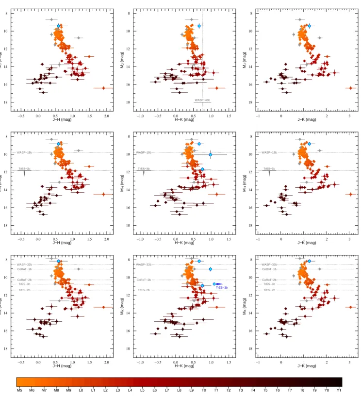
(2012) and references therein) but very few planets. Each of Figure 3’s panels contain WASP-12Ab, the only planet with firm detections of its emission in each of those near-infrared bands (MJ = 9.42, MH = 8.83, MKs = 8.16). A
few more measurements were obtained on individual sys-tems, but often in only one band (depicted as dotted lines). WASP-12Ab’s location seems to agree well with the top of the ultra-cool dwarf distribution especially in the J−H colour. The two colours involving the KS-band would imply
that the object is redder than most late M-dwarfs. However, a recent work byRogers et al. (2013) showed that eclipse depth measurements, notably in the KS bandpass are likely
to be biased towards deeper values. This in turns would make authors infer brighter planets, leading to a smaller magnitude and a redder colour index. Bean et al. (2013) observed WASP-19b at low spectral resolution and consis-tently found shallower occultation depths than broad band measurements would imply.
It remains unclear whether irradiated planetary atmo-sphere should follow the same general behaviour that very low-mass stars and field brown dwarfs have, whether they would constitute their own sequence or agree with a black-body (see Sec.4for a discussion on the matter). If indeed, ir-radiated planets and ultra-cool dwarfs were to coincide, then positioning a new measurement in a colour-magnitude dia-gram will become an efficient method to verify anyone’s re-sults. For instance, it can immediately be noticed how most KSbands results imply redder colours than would otherwise
be anticipated.
By extension, obtaining a detection in one band would offer straight-forward predictions for the other two bands. As an example, WASP-19b has an absolute magnitude in the H-band, MH = 9.80 ± 0.21 (Tab. B5). Reading on
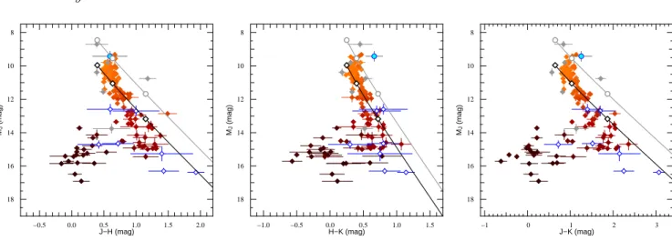
−0.5 0.0 0.5 1.0 1.5 2.0 8 10 12 14 16 18 J−H (mag) MJ (mag) . . . . WASP−43b −1.0 −0.5 0.0 0.5 1.0 1.5 8 10 12 14 16 18 . . . . H−K (mag) MJ (mag) −1 0 1 2 3 8 10 12 14 16 18 J−K (mag) MJ (mag) . . . . WASP−19b TrES−3b −0.5 0.0 0.5 1.0 1.5 2.0 8 10 12 14 16 18 J−H (mag) MH (mag) . . . . WASP−19b TrES−3b −1.0 −0.5 0.0 0.5 1.0 1.5 8 10 12 14 16 18 H−K (mag) MH (mag) . . . . WASP−19b TrES−3b −1 0 1 2 3 8 10 12 14 16 18 J−K (mag) MH (mag) . . . . TrES−3b CoRoT−1b TrES−2b CoRoT−2b WASP−33b −0.5 0.0 0.5 1.0 1.5 2.0 8 10 12 14 16 18 . . . . J−H (mag) MK (mag) TrES−3b TrES−2b WASP−33b CoRoT−2b −1.0 −0.5 0.0 0.5 1.0 1.5 8 10 12 14 16 18 H−K (mag) MK (mag) . . . . TrES−2b TrES−3b WASP−33b CoRoT−1b CoRoT−2b −1 0 1 2 3 8 10 12 14 16 18 . . . . J−K (mag) MK (mag) M5 M6 M7 M8 M9 L0 L1 L2 L3 L4 L5 L6 L7 L8 L9 T0 T1 T2 T3 T4 T5 T6 T7 T8 T9 Y0 Y1
5
10
15
20
25
30
−10
−5
0
5
10
15
Figure 3. Near-infrared colour-magnitude diagrams, using the 2MASS photometric system (i.e., the J, H and KSbands). The blue dots show the dayside emission of transiting planets observed during occultation. Squares and arrows represent upper limits. Lines labelled with the name of a planet show the position of systems where colour or absolute magnitude is missing (not all cases are represented, for clarity). The coloured diamonds underlying the plots are brown dwarfs and directly imaged planets, whose magnitudes are listed in
Dupuy & Liu(2012). Colours represent the spectral class of the object, spanning from M5 (orange) to Y1 (black). Unclassified objects
with the M & L-dwarf sequence at J−H= 0.6 ± 0.1. This leads to MJ = 10.40 ± 0.23, that we can convert into an
apparent magnitude. WASP-19b can be predicted to have mJ = 17.60 ± 0.21, on a par with WASP-12Ab’s
measure-ment (Tab.B4).
3.3 Mid-infrared
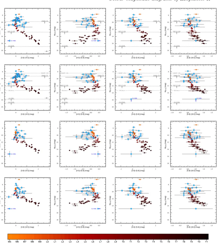
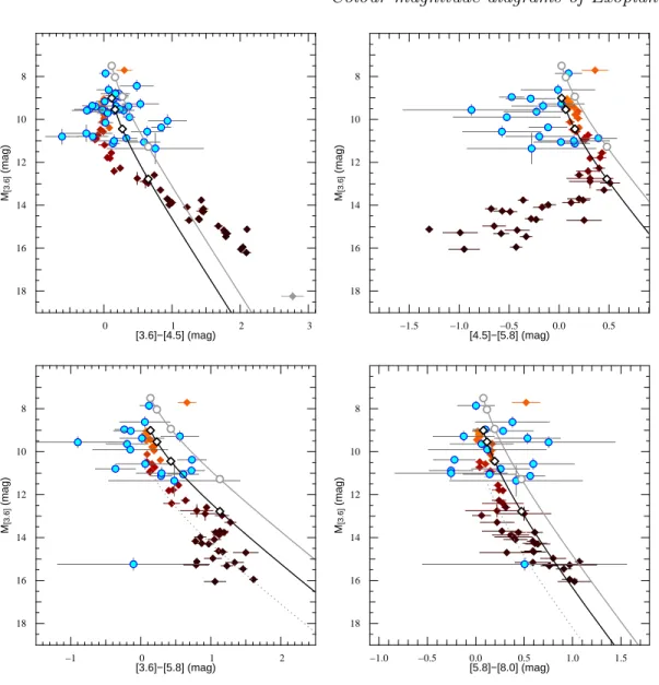
In the mid-infrared, all the bands that were considered are the Spitzer’s IRAC channels. Both ultra-cool dwarfs and exoplanets have been observed extensively, especially so in the IRAC 1 & 2 centred at 3.6 and 4.5 µm. Compared to the seven systems presented inTriaud(2014), the first diagrams in the top two rows in Fig.4show a marked increase in the number of objects.
3.3.1 [3.6]−[4.5]
The M & L-dwarf sequence is colour-less in those bands. Objects get fainter for decreasing temperatures. As brown dwarfs transition towards the T sequence, a sharp turn oc-curs, caused by the widening and deepening methane ab-sorption band at 3.3µm, revealed by the recession of dust clouds in brown dwarfs’ atmospheres (e.g.Patten et al. 2006, and references therein). This leads to increasingly redder colours with increasing magnitudes. The clarity of this pat-tern is handy to compare planets and brown dwarfs together. So far no planet that has had its emission detected clearly falls within the T-range. Good contenders can be found in HAT-P-12b (Hartman et al. 2009) whose upper limit places it beyond the methane kink and in WASP-80b that has a reported effective temperature around 800 K (Triaud et al.
2013a; Mancini et al. 2014). All currently measured hot
Jupiters can therefore be compared to the M & L sequence (GJ 436b, a Neptune, is kept aside for now).
Despite significant scatter, one can notice that objects are not located completely at random. No object redder than [3.6]−[4.5] = 1 for example exists. All planets but two have colours compatible or redder than brown dwarfs. This gets clearer for absolute magnitudes in the redder channels. Only GJ 436b ([3.6]−[4.5] < 0.6) and WASP-8Ab ([3.6]−[4.5] = 0.6) are significantly bluer, two eccentric planets (a third eccentric planet, HAT-P-2b ([3.6]−[4.5] = 0), is compatible with the colourless L-sequence).
The scatter in colour increases for increasing magni-tudes: objects brighter than the median magnitude (GJ 436b removed) consistently have an RMS in colour lower than ob-jects fainter than the median magnitude. This is not because intrinsically fainter planets produce weaker (and harder to measure) occultations. Some of the most significant detec-tions (for instance HD 189733Ab (M[3.6]= 11.1, [3.6]−[4.5]
= 0.1), HD 209458b (M[3.6] = 10.4, [3.6]−[4.5] = 0.8)) are
amongst the fainter planets. The graphs shuffled borderline and significant measurements by using absolute magnitudes. A clear detection arises because the host star and the planet are bright in apparent magnitudes, for instance thanks to their proximity to the Solar system.
The known hot Jupiters’ diversity in radius (0.8 to 2 Rjup), which does not exist for field brown dwarfs, cannot
be held responsible for the scatter either. A change in ra-dius translates with a decrease in absolute magnitude, but
no change in colour as shown in Fig. 6 when we compare with blackbodies, the current effects are much larger. This forces us to turn to other processes such as an increased di-versity (in atmospheric structure or in absorbents) at colder temperatures, or to some intrinsic variability (with an ampli-tude ∼ 1.5 mag). If such is the case, repeated measurements should be attempted.
3.3.2 [4.5]−[5.8]
Brown dwarfs face a similar pattern than in the previous subsection, but orientated in the opposite direction. It also marks the transition between the L and T spectral classes. With decreasing temperatures, CO (that has absorption in the IRAC 2 bandpass) reacts with H2 to produce CH4, it
also produces H2O that has several important absorption
features around 5.8µm. This makes the atmosphere become increasingly bluer with decreasing effective temperature.
The hot Jupiters, again, are all located in the abso-lute magnitude range of the M & L-sequence. Apart from GJ 436b, all are marginally bluer than their ultra-cool dwarf counterparts. Would we consider each planet individually, we would conclude that each is consistent with the M & L-sequence when in fact the general population clearly is not. It is systematically biased towards the blue: They have a mean colour inferior to 0 when all brown dwarfs are above 0 in the same absolute magnitude range. Water absorption has been noticed in several transmitted spectra (e.g.Deming
et al. 2013), which would indicate that planets may depart
from ultra-cool dwarfs’ atmospheres in that water absorp-tion appears at higher temperatures.
Alternatively planetary atmospheres and ultra-cool dwarfs could be reconciled if ultra-cool dwarfs contain an absorbant around 4.5 µm that planets do not possess. If present, it would increase the planets’ absolute magnitudes in the IRAC 2 channel at 4.5 µm, moving each point closer to 0.
3.3.3 [3.6]−[5.8] & [5.8]−[8.0]
Those two colours show a redward trend with decreasing lu-minosity. At [3.6]−[5.8] and at [5.8]−[8.0] planets and ultra-cool dwarf overlap very well: as many objects are found on either side of the brown dwarf sequence showing statisti-cal agreement. Planets may be slightly offset towards redder colours, in [5.8]−[8.0] but only marginally so at the moment. This agreement between planets and ultra-cool dwarfs could in principle act as a sort of calibration, validating that measurements in those bands are well estimated (in value and error bar). However, we have to remember here that hot Jupiters are significantly larger than the typical brown dwarf (∼ 1.3–1.6 Rjupvs 0.8–0.9 Rjup). Reducing the planets size
to the brown dwarf level should normally lead the planets to be dimmer by 0.8 to 1.5 magnitudes (see Fig.6and Sec.
4). At first sights, both classes of objects should not be compatible. The fact that both groups have similar absolute magnitudes, indicates that hot Jupiters have lower surface emissivity than ultra-cool dwarfs.
GJ 436b GJ 1214b HAT−P−12b Kepler−7b 0 1 2 3 8 10 12 14 16 18 . . . . [3.6]−[4.5] (mag) M [3.6] (mag) GJ 436b GJ 1214b HAT−P−12b Kepler−7b −1.5 −1.0 −0.5 0.0 0.5 8 10 12 14 16 18 [4.5]−[5.8] (mag) M [3.6] (mag) . . . . GJ 1214b HAT−P−12b Kepler−7b −1 0 1 2 8 10 12 14 16 18 . . . . [3.6]−[5.8] (mag) M [3.6] (mag) GJ 1214b HAT−P−12b Kepler−7b −1.0 −0.5 0.0 0.5 1.0 1.5 8 10 12 14 16 18 . . . . [5.8]−[8.0] (mag) M [3.6] (mag) GJ 436b GJ 1214b HAT−P−12b 55 Cnc e WASP−17b Kepler−7b 0 1 2 3 8 10 12 14 16 18 . . . . [3.6]−[4.5] (mag) M [4.5] (mag) GJ 436b GJ 1214b HAT−P−12b 55 Cnc e WASP−17b Kepler−7b −1.5 −1.0 −0.5 0.0 0.5 8 10 12 14 16 18 . . . . [4.5]−[5.8] (mag) M [4.5] (mag) GJ 436b GJ 1214b HAT−P−12b 55 Cnc e WASP−17b Kepler−7b −1 0 1 2 8 10 12 14 16 18 . . . . [3.6]−[5.8] (mag) M [4.5] (mag) GJ 436b GJ 1214b HAT−P−12b 55 Cnc e WASP−17b Kepler−7b −1.0 −0.5 0.0 0.5 1.0 1.5 8 10 12 14 16 18 . . . . [5.8]−[8.0] (mag) M [4.5] (mag) GJ 436b 0 1 2 3 8 10 12 14 16 18 . . . . [3.6]−[4.5] (mag) M [5.8] (mag) GJ 436b −1.5 −1.0 −0.5 0.0 0.5 8 10 12 14 16 18 . . . . [4.5]−[5.8] (mag) M [5.8] (mag) −1 0 1 2 8 10 12 14 16 18 . . . . [3.6]−[5.8] (mag) M [5.8] (mag) −1.0 −0.5 0.0 0.5 1.0 1.5 8 10 12 14 16 18 . . . . [5.8]−[8.0] (mag) M [5.8] (mag) GJ 436b 0 1 2 3 8 10 12 14 16 18 . . . . [3.6]−[4.5] (mag) M [8.0] (mag) GJ 436b −1.5 −1.0 −0.5 0.0 0.5 8 10 12 14 16 18 . . . . [4.5]−[5.8] (mag) M [8.0] (mag) −1 0 1 2 8 10 12 14 16 18 . . . . [3.6]−[5.8] (mag) M [8.0] (mag) −1.0 −0.5 0.0 0.5 1.0 1.5 8 10 12 14 16 18 . . . . [5.8]−[8.0] (mag) M [8.0] (mag) M5 M6 M7 M8 M9 L0 L1 L2 L3 L4 L5 L6 L7 L8 L9 T0 T1 T2 T3 T4 T5 T6 T7 T8 T9 Y0 Y1
5
10
15
20
25
30
−10
−5
0
5
10
15
Figure 4. Mid-infrared colour-magnitude diagrams, using Spitzer’s IRAC photometric system. The blue dots show the dayside emission of transiting planets observed during occultation. Squares and arrows represent upper limits. Lines labelled with the name of a planet show the position of systems where colour or absolute magnitude is missing (not all cases are represented, for clarity). The coloured diamonds underlying the plots are ultra-cool dwarfs and directly imaged planets, whose magnitudes are listed inDupuy & Liu(2012). Colours represent the spectral class of the object, spanning from M5 (orange) to Y1 (black). The only unclassified object here, in grey, is WD 0806-661B (Luhman et al. 2012).
−0.5 0.0 0.5 1.0 1.5 2.0 8 10 12 14 16 18 J−H (mag) MJ (mag) . . . . −1.0 −0.5 0.0 0.5 1.0 1.5 8 10 12 14 16 18 H−K (mag) MJ (mag) . . . . −1 0 1 2 3 8 10 12 14 16 18 J−K (mag) MJ (mag) . . . .
Figure 5. Same diagrams as the top line in Fig.3but showcasing the behaviour of blackbodies at 10 pc, whose effective temperature is changed while keeping its size constant. The plain grey line is for a 0.9 RJupobject, similar to the radius of a brown dwarf, and the plain black line represents a 1.8 RJup, the size of WASP-12Ab. The white-filled dots (0.9 RJup) and diamonds (1.8 RJup) along the blackbodies indicate the location of a 4 000, 3 000 and 2 000 K object. For reference, the blue, empty diamonds highlight the position of young, directly detected exoplanets whose data is located in TableB1.
3.3.4 Summary from mid-IR colours
If a reason is found to explain the apparent agreement at [3.6]−[5.8] & [5.8]−[8.0] then we could conclude that the 4.5 µm band measurements are at the source of the observed divergence between irradiated gas giants and brown dwarfs in the [3.6]−[4.5] & [4.5]−[5.8] colours. Introducing some additional absorber within the planets’ spectrum, around 4.5 µm, would move planets closer to 0 in both diagrams while keeping the [3.6]−[5.8] & [5.8]−[8.0] untouched. The fact that the intrinsically fainter planets display a greater di-vergence from the ultra-cool dwarfs in colours based on the 4.5 µm band, may imply that they have an increased atmo-spheric diversity, some of them with, and some without that absorbant. We prefer this interpretation over intrinsic vari-ability whose otherwise required amplitude would seem too large to explain the data. The discrepant [4.5] band has been noticed by a number of authors, withKnutson et al.(2009) proposing that a inversion in the temperature-pressure profile is responsible (Fortney et al. 2008). How-ever this interpretation has been disputed byMadhusudhan
et al. (2011), who argue that disparities in relative
abun-dances, notably the carbon to oxygen ratio, can reproduce the observations equally well.
A number of other measurements exists, notably ob-served in narrow bands (Gillon et al. 2009;Smith et al. 2011;
Crossfield et al. 2012;Gillon et al. 2012;Lendl et al. 2013;
Anderson et al. 2013), in the z’ band (L´opez-Morales et al.
2010; Lendl et al. 2013; Abe et al. 2013) or observed by
folding the CoRoT and Kepler lightcurves (e.g.Snellen, de
Mooij & Albrecht(2009);Alonso et al.(2009);Morris,
Man-dell & Deming(2013);Demory et al.(2013);Sanchis-Ojeda
et al.(2013)). Because of a lack of measured brown dwarfs
to compare them to and often, because of a lack of apparent magnitudes in those particular bands, it seemed futile to do this exercise at this time. It will however become something worth investigating.
4 COMPARISON WITH BLACKBODIES Hot Jupiter emission measurements are often compared to complex models and to blackbodies, with frequent claims that planet spectra are compatible with the shape expected of a blackbody. WASP-12Ab is one of the most noticeable ex-amples (Crossfield et al. 2012).Hansen, Schwartz & Cowan
(2014) surveyed the literature for objects whose emission has been detected in several datasets at the same wavelength and, taking the variation in results as a systematic error bar, found that planets have featureless spectra resembling blackbodies.
To answer this claim, and also because we should not expect irradiated planets and ultra-cool dwarfs to be ex-actly the same, plotting the location of blackbodies within a colour-magnitude diagram seemed warranted. The black-body loci can provide context by revealing how brown dwarfs depart from a blackbody and how irradiated gas giants com-pare to these departures. Figs.5and6have a 0.9 RJupand
a 1.8 RJup sized black-body plotted for all temperatures
between 4 000 and 400 K. Those sizes where chosen as they represent the maximum size brown dwarfs are expected to have (with an age > 1 Gyr; Baraffe et al. 2003), and the approximate size of WASP-12Ab, one of the largest known exoplanet.
If planets were blackbodies their measurements should be comprised strictly between the 0.9 and 1.8 RJup
black-bodies. They cannot be above and cannot be below that strip (except for HD 149026b and GJ 436b). In the near-infrared (the only transiting planet in Fig. 5) and mid-infrared, WASP-12Ab is lying near or on top of the ex-pected blackbody line, in absolute magnitude and colour. Its location is also slightly above the 3 000 K mark, which is compatible with its estimated equilibrium temperature of 2 990 ± 110 K as provided byCrossfield et al.(2012).
Whether WASP-12Ab follows the behaviour of a late M dwarf better than a blackbody is irrelevant in this case: in all colours, the M & L sequence intersects with the ex-pected blackbody line at WASP-12Ab’s location in the
0 1 2 3 8 10 12 14 16 18 [3.6]−[4.5] (mag) M[3.6] (mag) . . . . −1.5 −1.0 −0.5 0.0 0.5 8 10 12 14 16 18 [4.5]−[5.8] (mag) M[3.6] (mag) . . . . −1 0 1 2 8 10 12 14 16 18 [3.6]−[5.8] (mag) M[3.6] (mag) . . . . . . . . −1.0 −0.5 0.0 0.5 1.0 1.5 8 10 12 14 16 18 [5.8]−[8.0] (mag) M[3.6] (mag) . . . .
Figure 6. Same diagrams as the top line in Fig.4but showcasing the behaviour of blackbodies at 10 pc whose effective temperature is changed while keeping its size constant. In plain grey, is drawn a 0.9 RJupobject, similar to the radius of a brown dwarf, and in plain black a 1.8 RJup, the size of WASP-12Ab. The two bottom panels have an added dotted grey line, which is a blackbody the size of GJ 436b (0.38 RJup). The marks along the blackbodies indicate the expected location of a 4 000, 3 000, 2 000 and 1 000 K object.
colour-magnitude diagram3. The planet is where it ought
to be. Having only few examples to work with, we added to Fig. 5 the directly imaged planets (Table B1). Apart from the recently announced GU Psc b (Naud et al. 2014), those young planets show good agreement with their M & L-dwarf counter parts, but continue redder and fainter in-stead of turning into the blueward L-T transition, not unlike grey atmospheres. Irradiated planets could follow blackbod-ies, the ultra-cool dwarf’s sequence, the path of the young directly imaged planets, or their own sequence. To differen-tiate between these four solutions, measurements of cooler transiting planets are required in near-infrared bands. HAT-P-12b and WASP-80b are good contenders.
In the mid-infrared, the picture is more complex. In the
3 reflected light likely plays no part in placing WASP-12Ab at this special location. It is expected to be about three orders of magnitude fainter than thermal emission (Seager & Deming 2010)
M[3.6]vs [3.6]−[4.5] diagram, there are seven planets redder
or brighter than the 1.8 RJupblackbody. Thirteen systems
are bluer or fainter than the 0.9 RJup blackbody. Due to
the dispersion (increasing with increasing magnitude), nei-ther the brown dwarfs, nor the blackbodies would seem to better explain all the measurements. We note that only two systems are more than 1σ above the 1.8 RJup blackbody
(HD 209458b and XO-4b), and one (WASP-8Ab) is away from the brown dwarfs. All other gas giants lie in agreement with a triangular confinement bordered by the blackbody on one side and the ultra-cool dwarf atmospheres on the other two. Targeting planets at the cool junction between the T-dwarfs and the blackbody expectations will show if planets follow the T-sequence, a blackbody, or their own se-quence (for example when reflected starlight starts produc-ing a strong effect). This means studyproduc-ing gas giants cooler than 1 000 K (whose size would presumably be closer to 0.9 than 1.8 RJup).
The M[3.6] vs [4.5]−[5.8] diagram shows that the
L-sequence is slightly brighter than a 0.9 RJup blackbody
would predict, but generally follows the same slope. Brown dwarfs clearly depart when they transition to the T spec-tral class. In section3.3.2we noted the blueward bias of hot Jupiters. This is strengthened when compared to a black-body. Planets clearly depart. If each measurement is only 1 to 2σ away, what we lack in precision we gain in the num-ber of systems measured. Hot Jupiters are not featureless. Again here, the departure between the brown dwarfs and the blackbody happens below 1 000 K.
Gas-giants and ultra-cool dwarfs agree well in M[3.6]
vs [3.6]−[5.8]. However planets do not match the expecta-tions of a blackbody: All but four planets are found bluer or fainter than the 0.9 RJup blackbody line. The fact that
planets follow the same slope as a blackbody suggests a be-haviour similar to a grey atmosphere, implying that opac-ities in these bands are grey. Hot-Jupiters are not black-bodies and here behave more like dwarfs do. The final dia-gram, plotting M[3.6] vs [5.8]−[8.0] shows good agreement:
brown dwarfs appear to follow the expected blackbody (be-ing slightly below, maybe evidence they are slightly smaller than 0.9 RJup), so do hot Jupiters but with a large scatter.
This would indicate that the opacity is grey in these bands and approach Planck’s law.
The location of a blackbody with the size of GJ 436b (0.38 RJup) was added and goes right through its
measure-ment at [5.8]-[8.0]. A change in radius is only a transla-tion in absolute magnitude. GJ 436b sits right at the 1 000 K marks, which would imply a similar temperature, much higher than its estimated equilibrium temperature of ∼700
K (Deming et al. 2007). If this is not the indication of
ex-cess energy produced by its on-going tidal circularisation
(Maness et al. 2007;Beust et al. 2012), this should be seen
as a reminder that effective temperature is different from equilibrium temperature and that touching the blackbody sequence, does not mean a measurement agrees with it, as temperature too needs to be accounted for. Shape is not all.
5 DISCUSSION & CONCLUSION
We computed photometric distances that allowed us to ob-tain the absolute magnitude of occulting planets. They were used to compile colour-magnitude diagrams. Planets on their own would not offer much information. This is why we com-pared their location in these diagrams, to the location of very low-mass stars and field brown dwarfs, and to the be-haviour expected of pure blackbodies. By defining a black-body sequence with a lower size of 0.9 RJup and an upper
one of 1.8 RJup, we describe a locus in the form of a strip
where all hot Jupiters should congregate would they follow Planck’s law.
In the near-infrared, three clear conclusions can be drawn:
• Planets are brighter in KS band measurements, and in
average redder than the M & L brown dwarf sequence (this probably has an instrumental origin).
• WASP-12Ab is as much compatible with a blackbody as with the M & L sequences, because that is the location where both intersect.
• A clear distinction between irradiated gas giants fol-lowing a brown dwarf behaviour, the young directly-imaged planets, or a blackbody will emerge for equilibrium temper-atures cooler than ∼ 2 000 K.
In the mid-infrared we obtained the following general trends:
• Gas giants are only in agreement with the blackbody locus in the [5.8]−[8.0] colour. Deviations, made significant by the number of objects considered, in the other colours imply that planet are not pure blackbodies, although indi-vidual objects may appear to be.
• Gas giants are bluer in the [4.5]−[5.8] colour than a blackbody or the M & L brown dwarf sequence. This shows that hot Jupiters are not featureless.
• Combining this with an increased scatter as magnitudes increase in the [3.6]−[4.5], provides support that some gas giants are missing an absorbant at 4.5 µm.
• This affects only certain planets making us conclude that atmospheric diversity increases with decreasing abso-lute magnitude, presumably, with decreasing equilibrium temperature.
• Clearly associating planets to the brown dwarf locus or to the blackbody strip can be made by obtaining the emission (dayside or nightside) of gas giants with effective temperatures below 1 000 K at [3.6] and [4.5].
It is worth noting at this point that the observed in-crease in atmospheric diversity is found under the upper limits placed by Demory et al. (2013) on Kepler-7b. This planet’s detected occultation and phase curve in the Ke-pler bandpass have been interpreted as reflected light from an inhomogeneous, high albedo, cloud layer, mostly located on the dayside. From studying HD 189733Ab’s phase curve inside a colour-magnitude diagram, Triaud (2014) made a similar inference: the presence of clouds can hide the effect of some absorbing species, or can locally change the atmo-spheric chemistry. We can therefore wonder whether the ex-istence of clouds can be linked to the presence or absence of an absorbing feature in Spitzer’s 4.5 µm channel that leads to the scatter present in the [3.6]−[4.5] and [4.5]−[5.8] colours.
If brown dwarf atmospheres and irradiated exoplanets are set to coincide, then it is perhaps not surprising that since most exoplanets fall in the range occupied by the M & L types, they too would have an opaque cloud layer at least on the dayside. Clouds are likely to leak over the termina-tor covering transmitted features. This provides context to the frequently announced featureless transmission spectra on several exoplanets (e.g. Bean, Miller-Ricci Kempton &
Homeier 2010; Berta et al. 2012; Sing et al. 2013; Jord´an
et al. 2013). GJ 436b is found on the continuation of the
M & L sequences, and too shows a featureless transmis-sion spectrum (Knutson et al. 2014). The scatter in colour of the emitted spectra for the colder of the transiting gas giants can give hope that some will possess an inhomoge-neous cloud cover, revealing the deeper parts of their at-mospheres through cloud holes. Using colour-magnitude di-agrams would become a useful tool to select the right ex-oplanet sample before attempting an observing campaign aimed at producing transmission spectra.
sup-plementary materials, that for an equivalent emerging flux, the spectra of an irradiated and of an isolated planet are dissimilar, notably by possessing widely different temperature-pressure profiles. The widening range in colour could also originate from distinctions in the impacting irra-diative stellar flux, or on how this energy affects different atmospheres. An irradiated planet, for instance emits more strongly at 4.5 µm than its isolated equivalent.
An obvious extension of this work would be to explore other colours, notably in some narrow bands where success-ful occultations measurements have been obtained by a num-ber of investigators. Ultra-cool dwarf magnitudes can be obtained from the many spectra that have been acquired of these objects and integrating over the correct bandpasses. It would be interesting to know whether those fall into regions sensitive to additional species, which could greatly help our understanding of exoplanetary atmospheres. For instance,
Demory et al. (2013) have shown how bright Kepler-7 is
in Kepler’s optical bandpass, Kmag, compared to its mid-infrared magnitude. It is therefore likely that a Kmag-[3.6] or a Kmag-[4.5] would be a tracer of cloudy structures on the dayside of exoplanets. We cannot but encourage authors to report apparent magnitudes in the bands that they report occultations in.
From studying those diagrams we can make judgements about the most interesting planets to obtain emission mea-surements on. Some objects are particular in deviating from the global trends we outlined above, with the clearest ex-ample found with GJ 436b. Its small size is not sufficient to explain its discrepancy. The absence of a detection in the 4.5 µm band signifies it is the bluest object in the current sample in the [3.6]−[4.5] colour, and the reddest in [4.5]−[5.8]. While being broadly consistent with the shape of a blackbody, its inferred effective temperature (∼ 1 000 K) appears unreason-ably high. The study of the other smaller planets, GJ 1214 b
(Charbonneau et al. 2009), GJ 3470 b (Bonfils et al. 2012)
and HD 97658b (Dragomir et al. 2013) can show if they man-ifest an atmospheric behaviour similar to GJ 436b’s.
Arguably there are now enough measurements over the M & L sequences; it is scientifically interesting to reserve our ressources to extend beyond that range. Going further up along the M sequence would need hot Jupiters orbiting A stars (like WASP-33 (Collier Cameron et al. 2010;Deming
et al. 2012)) that are hard to come about and hard to
anal-yse: many A stars are within the instability strip and display oscillations (WASP-33 is a δ Scuti). Exploring further down, closer to the T regime, especially for equilibrium tempera-tures below 1 000 K can be achieved by targeting longer period planets (WASP-8Ab for example is close to the L-T transition (Queloz et al. 2010;Cubillos et al. 2013)). The main issue in observing colder planets are the weak signals that can be expected from them. This can be mitigated by selecting host stars of late spectral classes such as WASP-80
(Triaud et al. 2013a).
So far very few transiting (or occulting) brown dwarfs have been detected (Deleuil et al. 2008; Anderson et al.
2011a; Bouchy et al. 2011; Siverd et al. 2012; D´ıaz et al.
2013). Orbiting hot, and large stars their occultation can be hard to obtain, but are doable (Beatty et al. 2014). However, those brown dwarfs are mostly found on short orbits, like hot Jupiters. They have inferred temperatures similar to M or
L objects but differ from usual brown dwarfs in that they are inflated. Because of their size, they fall on isochrones younger than the inferred age of the star they orbit (Triaud
et al. 2013b). Proximity acts like a rejuvenation. Obtaining
several brightness measurements over the M, L and T range, preferably on long period objects would in principle procure a radius calibration for field brown dwarfs.
ACKNOWLEDGMENTS
The authors would like to thank Franck Selsis, Mercedes L´opez-Morales, Jacqueline Radigan, Mickael Bonnefoy, Josh Winn, Kevin Schlaufman and Jay Pasachoff for inspiring re-flections, for explanations – for reminders – and for providing comments and reactions to the text. We would like to also thank and acknowledge the influence of our referee, Hans Deeg, whose suggestions improved the paper and helped clarify it.
A. H. M. J. Triaud is a Swiss National Science Founda-tion fellow under grant number P300P2-147773.
This publication makes use of data products from the following projects, which were obtained through theSimbad
andVizieRservices hosted at theCDS-Strasbourg: • The Two Micron All Sky Survey (2MASS), which is a joint project of the University of Massachusetts and the Infrared Processing and Analysis Center/California Insti-tute of Technology, funded by the National Aeronautics and Space Administration and the National Science Foundation. • The Wide-field Infrared Survey Explorer (WISE), which is a joint project of the University of California, Los Angeles, and the Jet Propulsion Laboratory/California In-stitute of Technology, funded by the National Aeronautics and Space Administration.
• The Tycho2 catalog (Høg et al. 2000).
• The Amateur Sky Survey (TASS) (Droege et al. 2006). • The Fourth U.S. Naval Observatory CCD Astrograph Catalogue (UCA4) (Zacharias et al. 2013).
• The AAVSO Photometric All-Sky Survey (APASS), funded by the Robert Martin Ayers Sciences Fund.
We gathered the Spitzer Space Telescope data from the
Spitzer Heritage Archive. References to exoplanetary sys-tems were obtained by an extensive use of the paper repos-itories,ADSandarXiv, but also through frequent visits to theexoplanet.eu(Schneider et al. 2011) andexoplanets.org
(Wright et al. 2011) websites.
REFERENCES
Abe L. et al., 2013, A&A, 553, A49
Ackerman A. S., Marley M. S., 2001, ApJ, 556, 872 Alonso R. et al., 2008, A&A, 482, L21
—, 2004, ApJL, 613, L153
Alonso R., Deeg H. J., Kabath P., Rabus M., 2010, AJ, 139, 1481
Alonso R., Guillot T., Mazeh T., Aigrain S., Alapini A., Barge P., Hatzes A., Pont F., 2009, A&A, 501, L23 Anderson D. R. et al., 2011a, ApJL, 726, L19 —, 2008, MNRAS, 387, L4
—, 2011b, MNRAS, 416, 2108 —, 2013, MNRAS, 430, 3422
Anglada-Escud´e G., Rojas-Ayala B., Boss A. P., Wein-berger A. J., Lloyd J. P., 2013, A&A, 551, A48
Artigau ´E., Bouchard S., Doyon R., Lafreni`ere D., 2009, ApJ, 701, 1534
Bakos G. ´A. et al., 2011, ApJ, 742, 116 —, 2007a, ApJ, 670, 826
—, 2007b, ApJ, 656, 552
Baraffe I., Chabrier G., Allard F., Hauschildt P. H., 1998, A&A, 337, 403
Baraffe I., Chabrier G., Barman T. S., Allard F., Hauschildt P. H., 2003, A&A, 402, 701
Barge P. et al., 2008, A&A, 482, L17 Baskin N. J. et al., 2013, ApJ, 773, 124
Bean J. L., D´esert J.-M., Seifahrt A., Madhusudhan N., Chilingarian I., Homeier D., Szentgyorgyi A., 2013, ApJ, 771, 108
Bean J. L., Miller-Ricci Kempton E., Homeier D., 2010, Nature, 468, 669
Beatty T. G. et al., 2014, ApJ, 783, 112 Beerer I. M. et al., 2011, ApJ, 727, 23 Berta Z. K. et al., 2012, ApJ, 747, 35
Beust H., Bonfils X., Montagnier G., Delfosse X., Forveille T., 2012, A&A, 545, A88
Blecic J. et al., 2014, ApJ, 781, 116 —, 2013, ApJ, 779, 5
Bonfils X. et al., 2012, A&A, 546, A27 Bonnefoy M. et al., 2013, A&A, 555, A107 —, 2011, A&A, 528, L15
Bouchy F. et al., 2011, A&A, 525, A68 —, 2005, A&A, 444, L15
Burgasser A. J., Marley M. S., Ackerman A. S., Saumon D., Lodders K., Dahn C. C., Harris H. C., Kirkpatrick J. D., 2002, ApJL, 571, L151
Burke C. J. et al., 2007, ApJ, 671, 2115
Burrows A. S., Ostriker J. P., 2014, Proceedings of the National Academy of Science, 111, 2409
Butler R. P., Vogt S. S., Marcy G. W., Fischer D. A., Wright J. T., Henry G. W., Laughlin G., Lissauer J. J., 2004, ApJ, 617, 580
Caballero J. A. et al., 2007, A&A, 470, 903 C´aceres C. et al., 2011, A&A, 530, A5 Carson J. et al., 2013, ApJL, 763, L32 Charbonneau D. et al., 2005, ApJ, 626, 523 —, 2009, Nature, 462, 891
Charbonneau D., Brown T. M., Latham D. W., Mayor M., 2000, ApJL, 529, L45
Chauvin G., Lagrange A.-M., Dumas C., Zuckerman B., Mouillet D., Song I., Beuzit J.-L., Lowrance P., 2004, A&A, 425, L29
Christiansen J. L. et al., 2010, ApJ, 710, 97 Collier Cameron A. et al., 2007, MNRAS, 375, 951 —, 2010, MNRAS, 407, 507
Cox A. N., 2000, Allen’s astrophysical quantities
Croll B., Albert L., Lafreniere D., Jayawardhana R., Fort-ney J. J., 2010a, ApJ, 717, 1084
Croll B., Jayawardhana R., Fortney J. J., Lafreni`ere D., Albert L., 2010b, ApJ, 718, 920
Crossfield I. J. M., Barman T., Hansen B. M. S., Tanaka I., Kodama T., 2012, ApJ, 760, 140
Crossfield I. J. M. et al., 2014, Nature, 505, 654
Cubillos P. et al., 2013, ApJ, 768, 42 Cushing M. C. et al., 2011, ApJ, 743, 50
Cutri R. M., et al., 2012, VizieR Online Data Catalog, 2311, 0
Cutri R. M. et al., 2003, VizieR Online Data Catalog, 2246, 0
Dawson R. I., Fabrycky D. C., 2010, ApJ, 722, 937 de Mooij E. J. W., Brogi M., de Kok R. J., Snellen I. A. G.,
Kenworthy M. A., Karjalainen R., 2013, A&A, 550, A54 de Mooij E. J. W., de Kok R. J., Nefs S. V., Snellen I. A. G.,
2011, A&A, 528, A49
Deleuil M. et al., 2008, A&A, 491, 889 Delorme P. et al., 2013, A&A, 553, L5 Deming D. et al., 2012, ApJ, 754, 106
Deming D., Harrington J., Laughlin G., Seager S., Navarro S. B., Bowman W. C., Horning K., 2007, ApJL, 667, L199 Deming D. et al., 2011, ApJ, 726, 95
—, 2013, ApJ, 774, 95
Demory B.-O. et al., 2013, ApJL, 776, L25 —, 2011, A&A, 533, A114
Demory B.-O., Gillon M., Seager S., Benneke B., Deming D., Jackson B., 2012, ApJL, 751, L28
Demory B.-O., Seager S., 2011, ApJS, 197, 12 D´ıaz R. F. et al., 2013, A&A, 551, L9 Dragomir D. et al., 2013, ApJL, 772, L2
Droege T. F., Richmond M. W., Sallman M. P., Creager R. P., 2006, PASP, 118, 1666
Dupuy T. J., Liu M. C., 2012, ApJS, 201, 19 Enoch B. et al., 2011, AJ, 142, 86
Flower P. J., 1996, ApJ, 469, 355
Fortney J. J., Lodders K., Marley M. S., Freedman R. S., 2008, ApJ, 678, 1419
Fressin F., Knutson H. A., Charbonneau D., O’Donovan F. T., Burrows A., Deming D., Mandushev G., Spiegel D., 2010, ApJ, 711, 374
Gillon M. et al., 2014, A&A, 563, A21 —, 2009, A&A, 506, 359
—, 2010, A&A, 511, A3 —, 2007, A&A, 472, L13
Gillon M., Pont F., Moutou C., Bouchy F., Courbin F., Sohy S., Magain P., 2006, A&A, 459, 249
Gillon M. et al., 2012, A&A, 542, A4
Gillon M., Triaud A. H. M. J., Jehin E., Delrez L., Opitom C., Magain P., Lendl M., Queloz D., 2013, A&A, 555, L5 Hansen C. J., Schwartz J. C., Cowan N. B., 2014, ArXiv
e-prints
Hartman J. D. et al., 2009, ApJ, 706, 785 Hebb L. et al., 2009, ApJ, 693, 1920 —, 2010, ApJ, 708, 224
Heinze A. N. et al., 2013, ApJ, 767, 173 Hellier C. et al., 2009, Nature, 460, 1098 —, 2011, A&A, 535, L7
Henry G. W., Marcy G. W., Butler R. P., Vogt S. S., 2000, ApJL, 529, L41
Hertzsprung E., 1911, Publikationen des Astrophysikalis-chen Observatoriums zu Potsdam, 63
Høg E. et al., 2000, A&A, 355, L27
Johns-Krull C. M. et al., 2008, ApJ, 677, 657 Jord´an A. et al., 2013, ApJ, 778, 184 Joshi Y. C. et al., 2009, MNRAS, 392, 1532 Kirkpatrick J. D., 2005, ARA&A, 43, 195 Kirkpatrick J. D. et al., 2011, ApJS, 197, 19
Knapp G. R. et al., 2004, AJ, 127, 3553
Knutson H. A., Benneke B., Deming D., Homeier D., 2014, Nature, 505, 66
Knutson H. A., Charbonneau D., Allen L. E., Burrows A., Megeath S. T., 2008, ApJ, 673, 526
Knutson H. A., Charbonneau D., Burrows A., O’Donovan F. T., Mandushev G., 2009, ApJ, 691, 866
Knutson H. A. et al., 2012, ApJ, 754, 22 Kov´acs G. et al., 2007, ApJL, 670, L41 Lagrange A.-M. et al., 2009, A&A, 493, L21 Latham D. W. et al., 2009, ApJ, 704, 1107 —, 2010, ApJL, 713, L140
Latham D. W., Stefanik R. P., Mazeh T., Mayor M., Burki G., 1989, Nature, 339, 38
Laughlin G., Deming D., Langton J., Kasen D., Vogt S., Butler P., Rivera E., Meschiari S., 2009, Nature, 457, 562 Lendl M., Gillon M., Queloz D., Alonso R., Fumel A., Jehin
E., Naef D., 2013, A&A, 552, A2 Lewis N. K. et al., 2013, ApJ, 766, 95
L´opez-Morales M., Coughlin J. L., Sing D. K., Burrows A., Apai D., Rogers J. C., Spiegel D. S., Adams E. R., 2010, ApJL, 716, L36
Luhman K. L., Burgasser A. J., Labb´e I., Saumon D., Mar-ley M. S., Bochanski J. J., Monson A. J., Persson S. E., 2012, ApJ, 744, 135
Machalek P., Greene T., McCullough P. R., Burrows A., Burke C. J., Hora J. L., Johns-Krull C. M., Deming D. L., 2010, ApJ, 711, 111
Machalek P., McCullough P. R., Burke C. J., Valenti J. A., Burrows A., Hora J. L., 2008, ApJ, 684, 1427
Machalek P., McCullough P. R., Burrows A., Burke C. J., Hora J. L., Johns-Krull C. M., 2009, ApJ, 701, 514 Madhusudhan N., Mousis O., Johnson T. V., Lunine J. I.,
2011, ApJ, 743, 191
Magain P., Courbin F., Sohy S., 1998, ApJ, 494, 472 Mahtani D. P. et al., 2013, MNRAS, 432, 693 Mancini L. et al., 2014, A&A, 562, A126 Mandushev G. et al., 2007, ApJL, 667, L195
Maness H. L., Marcy G. W., Ford E. B., Hauschildt P. H., Shreve A. T., Basri G. B., Butler R. P., Vogt S. S., 2007, PASP, 119, 90
Marley M. S., Seager S., Saumon D., Lodders K., Ackerman A. S., Freedman R. S., Fan X., 2002, ApJ, 568, 335 Marois C., Macintosh B., Barman T., Zuckerman B., Song
I., Patience J., Lafreni`ere D., Doyon R., 2008, Science, 322, 1348
Maxted P. F. L. et al., 2013, MNRAS, 428, 2645
Maxted P. F. L., Koen C., Smalley B., 2011, MNRAS, 418, 1039
Mazeh T. et al., 2000, ApJL, 532, L55 McArthur B. E. et al., 2004, ApJL, 614, L81 McCullough P. R. et al., 2008, ArXiv e-prints —, 2006, ApJ, 648, 1228
Mohanty S., Jayawardhana R., Hu´elamo N., Mamajek E., 2007, ApJ, 657, 1064
Morris B. M., Mandell A. M., Deming D., 2013, ApJL, 764, L22
Naef D. et al., 2001, A&A, 375, L27 Naud M.-E. et al., 2014, ApJ, 787, 5 Noyes R. W. et al., 2008, ApJL, 673, L79 Nymeyer S. et al., 2011, ApJ, 742, 35
O’Donovan F. T. et al., 2007, ApJL, 663, L37
O’Donovan F. T., Charbonneau D., Harrington J., Mad-husudhan N., Seager S., Deming D., Knutson H. A., 2010, ApJ, 710, 1551
O’Donovan F. T. et al., 2006, ApJL, 651, L61 O’Rourke J. G. et al., 2014, ApJ, 781, 109 P´al A. et al., 2008, ApJ, 680, 1450 Patten B. M. et al., 2006, ApJ, 651, 502 Perryman M. A. C. et al., 2001, A&A, 369, 339 Pollacco D. et al., 2008, MNRAS, 385, 1576 Queloz D. et al., 2010, A&A, 517, L1
Radigan J., Jayawardhana R., Lafreni`ere D., Artigau ´E., Marley M., Saumon D., 2012, ApJ, 750, 105
Radigan J., Lafreni`ere D., Jayawardhana R., Artigau E., 2014, ArXiv e-prints
Reach W. T. et al., 2005, PASP, 117, 978
Rogers J., L´opez-Morales M., Apai D., Adams E., 2013, ApJ, 767, 64
Rogers J. C., Apai D., L´opez-Morales M., Sing D. K., Bur-rows A., 2009, ApJ, 707, 1707
Russell H. N., 1914a, Nature, 93, 227 —, 1914b, Nature, 93, 252
—, 1914c, Nature, 93, 281
Sahlmann J. et al., 2011, A&A, 525, A95
Sanchis-Ojeda R., Rappaport S., Winn J. N., Levine A., Kotson M. C., Latham D. W., Buchhave L. A., 2013, ApJ, 774, 54
Sato B. et al., 2005, ApJ, 633, 465
Schneider J., Dedieu C., Le Sidaner P., Savalle R., Zolo-tukhin I., 2011, A&A, 532, A79
Seager S., Deming D., 2010, ARA&A, 48, 631 Shannon C. E., 1949, Proc. IRE, 37, 10 Sing D. K. et al., 2013, MNRAS, 436, 2956 Siverd R. J. et al., 2012, ApJ, 761, 123 Smalley B. et al., 2010, A&A, 520, A56 Smith A. M. S. et al., 2012, A&A, 545, A93
Smith A. M. S., Anderson D. R., Skillen I., Collier Cameron A., Smalley B., 2011, MNRAS, 416, 2096
Snellen I. A. G., de Mooij E. J. W., Albrecht S., 2009, Nature, 459, 543
Southworth J., 2011, MNRAS, 417, 2166 Stetson P. B., 1987, PASP, 99, 191
Stevenson K. B. et al., 2012, ApJ, 754, 136 Street R. A. et al., 2010, ApJ, 720, 337
Todorov K., Deming D., Harrington J., Stevenson K. B., Bowman W. C., Nymeyer S., Fortney J. J., Bakos G. A., 2010, ApJ, 708, 498
Todorov K. O. et al., 2013, ApJ, 770, 102 —, 2012, ApJ, 746, 111
Torres G., Andersen J., Gim´enez A., 2010, A&ApR, 18, 67 Torres G. et al., 2007, ApJL, 666, L121
Torres G., Winn J. N., Holman M. J., 2008, ApJ, 677, 1324 Triaud A. H. M. J., 2014, MNRAS, 439, L61
Triaud A. H. M. J. et al., 2013a, A&A, 551, A80 —, 2013b, A&A, 549, A18
Tsuji T., 2002, ApJ, 575, 264
van Leeuwen F., 2007, A&A, 474, 653
Wang W., van Boekel R., Madhusudhan N., Chen G., Zhao G., Henning T., 2013, ApJ, 770, 70
Wheatley P. J. et al., 2010, ArXiv e-prints Wilson D. M. et al., 2008, ApJL, 675, L113
Wilson P. A., Rajan A., Patience J., 2014, ArXiv e-prints Winn J. N. et al., 2011, ApJL, 737, L18
Wright J. T. et al., 2011, PASP, 123, 412
Zacharias N., Finch C. T., Girard T. M., Henden A., Bartlett J. L., Monet D. G., Zacharias M. I., 2013, AJ, 145, 44
Zhao M., Milburn J., Barman T., Hinkley S., Swain M. R., Wright J., Monnier J. D., 2012a, ApJL, 748, L8
Zhao M., Monnier J. D., Swain M. R., Barman T., Hinkley S., 2012b, ApJ, 744, 122
APPENDIX A: OBTAINING CALIBRATED APPARENT MAGNITUDES WITH SPITZER Apparent magnitudes in all four IRAC bands are based on IRAC images calibrated by the standard Spitzer pipeline (version S18.18 or S18.25 depending on their availability at the time of the data reduction). They are delivered to the community as Basic Calibrated Data (BCD) sets and can be easily found at the Spitzer Heritage Archive4.
Accord-ing to the brightness of each targets, some sets were ob-served in the IRAC channels in sub-array mode, some in full-array mode and a number in both. This forced us to employ two different data reductions. The sub-array mode offers a high temporal resolution for observing very bright sources (available exposure times : 0.02, 0.1 and 0.4 seconds) on a portion of the array detector (32×32-pixel). The full-array mode provides 256×256-pixel (5.22’ × 5.22’) frames for longer exposure times of 2, 12, 30 and 100 seconds.
A1 Aperture photometry
Each BCD set provided by sub-array mode is composed of 64 sub-array images. These data are reduced according to the EXOPHOT pyraf pipeline following Lanotte et al. (in prep) to get raw light curves. For each sub-array image, a 2-D el-liptical Gaussian profile fit is performed on the point spread function (PSF) of the target to obtain its PSF centre co-ordinates. We operate aperture photometry thanks to the IRAF/DAOPHOT5 software (Stetson 1987). For each sub-array image, the software measures the stellar flux on apertures centred on our estimated PSF locations, ranging from 2.5 to 5.9 pixels by increments of 0.1 pixel, and subtracts the background level evaluated in an annulus extending from 12 to 15 pixels from the centre of aperture. For each block of 64 sub-array images, the discrepant values for the measure-ments of the x- and y-position, and the stellar and back-ground flux are rejected using a 3-σ median clipping. The remaining measurements in each BCD set are averaged.
The full-array mode images are reduced in the same way, except that the PSF centres are determined by a flux-weighted centroid. This method is better adapted to lower signal-to-noise data.
At this stage, the first measurements of each light curve are discarded if they correspond to deviant values for all or some of the the external parameters (detector or pointing
4 http://sha.ipac.caltech.edu/applications/Spitzer/SHA/ 5 IRAF is distributed by the National Optical Astronomy Obser-vatory, which is operated by the Association of Universities for Research in Astronomy, Inc., under cooperative agreement with the National Science Foundation.
stabilisation). Finally we perform for each light curve a mov-ing median filtermov-ing to discard outlier measurements due, for instance, to cosmic hits. We also reject the measurements during a planetary transit, if present, to always consider the total stellar flux. Ideally one should measure the flux coming from the stellar system only during the occultation of the planet to only consider the stellar flux. However the plane-tary emission is negligible in comparison to flux variations induced by instrumental effects such as the ‘pixel-phase’ and the ‘ramp’ effects. The first one lies in the dependence of the observed flux with the stellar centroid location on the pixel of the IRAC InSb (3.6 and 4.5 µm) arrays. It is due to the inhomogeneous intra-pixel sensitivity combined to the jitter of the telescope and to the poor sampling of the PSF. The second effect is the increase of the detector response at the start of AORs and is attributed to a charge-trapping mech-anism resulting in a dependence of the gain of the pixels to their illumination history. We refer the reader toKnutson
et al. (2008) and references therein for more informations
about these instrumental systematics.
The pixel phase response changed at the beginning of the Warm mission, with the consequence that the correction map of the cryogenic phase of Spitzer could not be used for all the data. Since no complete correction map is available for the Warm phase of Spitzer at the time of our analysis, we do not correct the flux measurements for the intra-pixel sensitivity. In practice, those intra-pixel flux variations are partially averaged out thanks to variations in the location of the PSF during an observational run. We do not model the ‘ramp’ effect but simply remove the more affected sequence of measurements.
For each dataset (called AOR = Astronomical Observa-tion Request in Spitzer terminology), we average all remain-ing measured stellar fluxes computed for each radius sepa-rately. We then apply the appropriate aperture correction to determine the stellar flux as it would be falling into a circular aperture radius of 10 pixels. This is carried out in order to remain consistent with the magnitude calibrations present in
Reach et al.(2005). The IRAC instrument handbook
pro-vides aperture corrections for different aperture radii and background annuli. However only three aperture corrections can be applied for the sub-array mode data, so that we generate other aperture correction factors to coincide with all our photometric apertures. Indeed the accuracy of the flux measurement resides in the choice of the photometric aperture radius. While small aperture radii are dominated by imprecisions due to under-sampling the PSF and pixel to pixel response, larger radii are affected by larger back-ground contributions. We thus perform aperture photometry on deconvolved images reconvolved by the best-fitting par-tial PSF model to derive the aperture corrections required for deriving the observed flux of the star. The deconvolution photometry is made using DECPHOT following a procedure described inGillon et al. (2006) and optimised for Spitzer data by Lanotte et al. (in prep). DECPHOT is based on the image-deconvolution method of Magain, Courbin & Sohy
(1998) that, contrarily to traditional deconvolution meth-ods, respects the sampling theorem ofShannon (1949) and preserves the photometric flux. The aperture corrections are normalised to the flux falling into a circular aperture radius of 10 pixels subtracted to the background level measured in an annulus from 12-20 pixels.
Table A1. Dilution factors in the stellar flux from CoRoT-2A and WASP-8A caused by their visual companion. These factors are estimated for a range of aperture radii.
Aperture radius Dilution (%) CoRoT-2A WASP-8A (pixels) [3.6] [4.5] [3.6] [4.5] 2.5 4.08 2.72 0.85 1.23 3.0 7.51 5.80 2.54 3.56 3.5 12.98 11.31 6.34 7.87 4.0 17.44 15.60 9.90 11.83 4.5 18.91 17.19 11.43 13.76
Then we average all flux corrected for aperture and take the resulting value as the observed flux measurement for the dataset. The mean of the errors on each corrected flux is taken as our error bar on the measured stellar flux. We convert the measured flux in Jansky and apply the colour and inter-pixel corrections6. Finally the flux densities are converted into Vega apparent magnitudes using the zero-magnitude flux densities computed byReach et al. (2005). The associated error bars are dominated by the uncertainty in the absolute calibration.
A2 Deconvolution of blended stars
Two systems in our sample (CoRoT-2 and WASP-8) are blended by a visual companion. Gillon et al. (2010) and
Deming et al. (2011) have evaluated the dilution factor:
the correction to the measured flux needed to remove the dilution caused by CoRotT-2A’s visual companion. Their correction factors at 4.5 µm return a magnitude disparity of ∼0.3 mag using our measured fluxes using the method de-scribed above. No similar work has been done for WASP-8. In order to measure the dilution factor induced in the flux measurement with a higher precision, we performed once again a deconvolution of the data for those two stars. We used DECPHOT to operate aperture photometry on model im-ages considering two stars or the target only. We compute the dilution factor for both systems using all our aperture radii to reduce the errors of the inferred factors. The stan-dard deviations of CoRoT-2 and WASP-8 fluxes due to the change of aperture radius are 0.11 and 0.07 %, respectively, at 3.6 µm, and 0.04 and 0.08 % at 4.5 µm. For comparison, the standard deviations of isolated target fluxes due to the change of aperture radius are encompassed between 0.01 and 0.06 %. Table A1 gives dilution factors according to some aperture radius, the target, and the instrument. With these factors, fluxes for each aperture are corrected and the same procedure as described in the previous section is carried out to yield corrected apparent magnitudes.
APPENDIX B: TABLES
6 see §4.4 and 4.5 of the Spitzer Observer’s Manual and http://irsa.ipac.caltech.edu/data/SPITZER/docs/irac/warmfeatures/
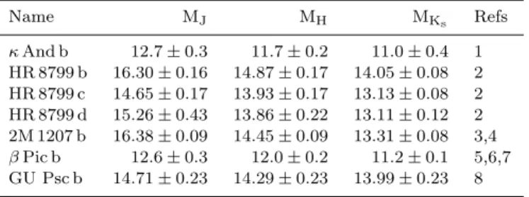
Table B1. Absolute magnitudes reported for some directly im-aged planets. Name MJ MH MKs Refs κ And b 12.7 ± 0.3 11.7 ± 0.2 11.0 ± 0.4 1 HR 8799 b 16.30 ± 0.16 14.87 ± 0.17 14.05 ± 0.08 2 HR 8799 c 14.65 ± 0.17 13.93 ± 0.17 13.13 ± 0.08 2 HR 8799 d 15.26 ± 0.43 13.86 ± 0.22 13.11 ± 0.12 2 2M 1207 b 16.38 ± 0.09 14.45 ± 0.09 13.31 ± 0.08 3,4 β Pic b 12.6 ± 0.3 12.0 ± 0.2 11.2 ± 0.1 5,6,7 GU Psc b 14.71 ± 0.23 14.29 ± 0.23 13.99 ± 0.23 8 References: (1)Carson et al.(2013); (2)Marois et al.(2008); (3)
Chauvin et al.(2004); (4)Mohanty et al. (2007); (5)Lagrange
et al. (2009); (6) Bonnefoy et al. (2011); (7) Bonnefoy et al.