PROCEEDINGS OF ECOS 2017 - THE 30TH INTERNATIONAL CONFERENCE ON EFFICIENCY, COST, OPTIMIZATION, SIMULATION AND ENVIRONMENTAL IMPACT OF ENERGY SYSTEMS
JULY 2-JULY 6, 2017, SAN DIEGO, CALIFORNIA, USA
1
Rule-based control and optimization of a hybrid
solar microgrid for rural electrification and heat
supply in sub-Saharan Africa
Queralt Altés Bucha, Matthew Oroszb, Sylvain Quoilinc and Vincent Lemortd
a University of Liège, Liège, Belgium, qaltes@ulg.ac.be b Massachusetts Institute of Technology, Cambridge, US, mso@mit.edu
c
University of Liège, Liège, Belgium, squoilin@ulg.ac.be
d University of Liège, Liège, Belgium, vincent.lemort@ulg.ac.be
Abstract:
This work aims at developing, optimizing and controlling a hybrid solar microgrid for rural electrification and heat supply in sub-Saharan Africa. The considered system includes PV panels, Parabolic Trough Collectors, ORC and LPG generator, as well as battery and thermal energy storage. A special focus is paid to the co-optimization of the thermal and electrical load satisfaction since it can improve the overall energy efficiency of the system. To that end, different sub-component models are developed:
- A building model to predict thermal loads of a health clinic in rural communities of Lesotho. - A microgrid model built by interconnecting the subcomponent models.
- A rule-based control strategy, dispatching heat and electrical powers of each component to cover the demand while minimizing the fuel consumption.
- A particle-swarm optimization of the microgrid under different cost assumptions.
For the studied community of Ha Nkau in Lesotho, the determined optimal system infrastructure is composed of PV (66 kW) and batteries (262 kWh), and the optimum control strategy achieves a levelized cost of electricity of 0.203 USD/kWh. Fuel consumption is mainly due to the burner, which supplies most of the thermal load together with CSP (66 m2) and TES (86 kWh).
Keywords:
Microgrid, Rule-Based Control, ORC, Particle-Swarm Optimization, Sub-Saharan Africa, Rural Electrification.
1. Introduction
Recent interest in small-scale solar thermal combined heat and power (CHP) power systems has coincided with demand growth for distributed electricity supplies in areas poorly served by centralized power stations. Potential technical approaches to meeting this demand are the parabolic trough solar thermal collector coupled with an Organic Rankine Cycle (ORC) heat engine, or in combination with solar photovoltaic (PV) panels.
This paper presents the dynamic simulation of a hybrid microgrid system. The studied configuration considers PV panels, Parabolic Trough Collectors (CSP), ORC and Liquefied Petroleum Gas (LPG) generation, as well as chemical battery storage and Thermal Energy Storage (TES).
The model, implemented in Python, iteratively evaluates configurations meeting variable demands (heat and electricity) according to an energy balance, calculates the microgrid cost structure based on cash flows, and seeks to minimize the levelized cost of energy. The energy balance is calculated at each timestep (user selectable with 1 h default) and a rule-based control logic directs the flows of energy between generation, storage and demand nodes. The control logic is formulated to reach decisions for the following possibilities:
Which combination of generators should be used to meet the loads? What is the optimum output level of selected generators?
2
For each configuration, the model allocates at each timestep the output of an available or combination of available generators to meet the load. A power outage condition due to insufficient generation is not permitted in the system, i.e. the micro-grid is designed to meet 100\% of demand, and will do so with backup fossil fuel generation if necessary. The complement of generators therefore always includes an LPG genset sized for the peak load of the microgrid.
To improve computational efficiency, some complex components have been implemented as functions derived from detailed models of those components. For example, the ORC performance is fitted from [1]. Similarly, thermal demands of a clinic and a school are represented as a time series derived from the model developed in [1].
1.1. Overall description
Fig. 1 describes the studied system. It presents the following features:
The electrical load can be met by the backup generator (operating with LPG or propane), the PV system, the ORC, the battery (via an inverter), or a combination of those.
The thermal load can be covered by the high temperature thermal energy storage (TES), the condenser of the ORC (in CHP mode) or by a backup burner.
The main heat source of the ORC is the CSP system through the thermal storage. The TES enables extended operating hours to times without solar irradiation.
The TES is charged by the CSP but also through the thermal potential of the exhaust gases of the LPG generator.
The ORC can also be used with the exhaust gases of the LPG generator as heat source in case no CSP system is installed.
The battery bank can be charged variously by the ORC, the PV or the backup generator.
Fig. 1. Hybrid micro-grid configuration (adapted from [2])
2. Electrical and thermal demands
Determining an accurate load demand profile is a key factor in order to obtain optimized micro-grid designs [3]. The case study considered in this work is based on on-going work in the community of Ha Nkau in the Mohale's Hoek District, Lesotho [2]. The community is currently without access to electricity and comprises 84 households, 5 small businesses, a school, a church and a health clinic. Electrical loads are obtained from an estimation tool developed in [2], which processes the data available from similar communities in a probabilistic distribution function. The annual load profile
3
for the case study is thereby obtained. The electrical demand of the clinic and the school is estimated from the available data from onsite monitoring campaigns [1].
In the considered system, the microgrid only supplies the thermal demand of the clinic and the school. This demand is evaluated using the physical building model developed in [1].
3. Modeling of generation systems
3.1. PV
PV generation depends on the temperature of the cells, which affects their efficiency. It is calculated according to [4] with a modified DNI to account for the latitude tilt. If the system is equipped with PV panels and if the solar irradiation is higher than the cut-off below which technology is not responsive, the PV power generation is calculated by [1] (equation 5.7). Otherwise, there is no power generation.
3.2. ORC
The ORC uses R245fa with a one-stage expansion, commercial HVAC tubes-and-fins air condenser and brazed plate heat exchangers for high pressure heat transfer [5]. The system power output is 3-5kWe [5], and currently does not accommodate thermal demand. In order to produce hot water for both sanitary needs and heating, the possibility of co-generation is offered by installing a condenser that works with water as a secondary fluid in addition to the current air-flow condenser [1].
The power output from the ORC mainly depends on the heat source (if there is a CSP installation, heat comes from TES; alternately, the ORC performs waste heat recovery (WHR) from the backup generator) but also, as mentioned above and described in [1], on the type of condenser that is being used (air- or water-flow). The ORC output power is computed in a different manner depending on the current case. These cases, which cover all possible system installations, are explained in a diagram in Fig. 2 (the boolean variables of the model are indicated in italic).
O
RC pow
er outpu
t
Configuration 1: ThereIsCSP and heatingORC
TES is the ORC heat source and ORC is the heating system
P
th
> 0 Case 1: There is heating demand
Water-flow condenser: PORC,el= f(Pnom,ORC, Wnet,wcd) and PORC,th = f(Pnom,ORC, Qcd,wcd)
P
th
< 0 Case 2: There is no heating demand
ORC uses the air-flow condenser: PORC,el= f(Pnom,ORC, Wnet,acd) and PORC,th = 0 Configuration 2: ThereIsCSP and heatingTES
TES is the ORC heat source and the heating system
ORC uses the air-flow condenser: PORC,el= f(Pnom,ORC, Wnet,acd) and PORC,th = 0
Configuration 3: not ThereIsCSP
WHR from the genset is the ORC heat source
P
th
> 0 Case 1: There is heating demand
Water-flow condenser: PORC,el= f(Pgenset, Tamb) and PORC,th = f(PORC,el, ηORC)
P
th
< 0 Case 2: There is no heating demand
ORC uses the air-flow condenser: PORC,el= f(Pgenset, Tamb) and PORC,th = 0
Fig. 2. Diagram of the ORC model
3.3. LPG generator: model and operation
The system features LPG-fuel generator as a backup for power generation. Ultimately, if there is insufficient power generation from renewable technologies, the generator must provide the balance of the load. Therefore, its nominal power is set equal to the peak load of the community.
4
The generator is only on when there is a residual load (RL) (i.e. PV is not supplying the entire load). In this case, the generator load is equal to the balance of demand after accounting for PV supply, taking into account any additional amount produced by the ORC (in the case where it is running). The possible cases (Configuration 1 and 2) are explained in the diagram in Fig. 3.
The generator output Pgenset,load is set to the value of the unmet load (according to current demand).
This load represents the minimum load the generator must supply. However, because the efficiency of LPG generators tends to drop abruptly in part-load operation, the generator load should be set to the highest possible value (i.e. ensuring no load is being dumped). The generator remaining capacity RC is therefore used to charge the batteries, if the latter are not full and according to its maximum charge capacity per timestep (Cases 1 and 2 in Fig. 3).
The genset fuel consumption is computed according to an efficiency curve extracted from its datasheet [6].
LPG genera
tor pow
er o
utput
Determine the residual load: RL = demand - PPV
Configuration 1: not ThereIsCSP and ThereIsORC
WHR from the genset is the ORC heat source. The ORC is always operating at the same time than the LPG generator. The generator load is lower than RL because the ORC is also contributing
Pgenset,load (equation 5.11 in [1]) Configuration 2: else
Either the ORC runs independently with CSP or there is no ORC Pgenset,load = RL - PORC
Determine the generator remaining capacity: RC = Pmax,genset - Pgenset,load
Determine the batteries charge rate limit: Pbat,availableCharge = Pbat,max,charge - PORC,ToBat
Case 1: RC > Pbat,availableCharge
The generator charges the battery to the limit: Pgenset,ToBat = Pbat,availableCharge
Case 2: RC ≤ Pbat,availableCharge
The generator charges the batteries up to its full residual capacity: Pgenset,ToBat = RC
Determine total generator power output: Pgenset = Pgenset,load + Pgenset,ToBat
Determine fuel consumption (ηmax = 19.87%): mfuel [kg]
Fig. 3. Diagram of the LPG generator model
4. Modeling and control of storage units
4.1. Electrical energy storage: Batteries
When operating the battery, the key constraint is the maximum power that can be charged or discharged at every timestep. Its value is function of the State of Charge (SOC) from the previous timestep and the charge/discharge power limit, a characteristic value of the batteries.
The possible charge/discharge mechanisms are accounted for in (1). A positive amount represents power flowing into the charge batteries (charging) and a negative amount represents power flowing out from the batteries (discharging).
(1)
Batteries cannot be charged/discharged beyond the available capacity (of each timestep) or the maximum charge/discharge power in a timestep (fixed value). The model checks all possible cases and corrects the balance if it is out-of-limits. The model is explained in a diagram form in Fig. 4.
5 B atteries ene rgy bala nc e Pb at > 0 Case 1: charging
Case 1.1: There is more energy to charge than the amount that can be charged (Pbat > Pbat,max,charge)
The maximum is charged and the rest is curtailed. Reasign powers: Pdumped = Pbat - Pbat,max,charge
Pbat= Pbat,max,charge
Case 1.2: All charging powers can be delivered to the batteries. There is no curtailed
generation. (Pbat ≤ Pbat,max,charge)
P
b
at
≤ 0
Case 2: discharging (note that the powers have negative values)
Pdumped = 0
Case 2.1: The energy available in the batteries is less than the demand (Pbat < Pbat,max,charge)
The discharge is set to the limit and the rest is provided by another system Pbat= Pbat,max,discharge
Case 2.2: All the energy needed can be sourced from the batteries and delivered by the
inverter. (Pbat ≥Pbat,max,charge)
Determine the batteries SOC at the end of the timsetep (90% efficiency of dis-/charging assumed) Fig. 4. Diagram of the batteries energy balance model
4.2. Thermal energy storage: TES tank
The thermal energy storage is a packed bed of quartzite in which the heat transfer fluid circulates - there is no phase change and only sensible storage of heat is considered. In order to simplify the model the TES tank is assumed to be at a uniform temperature. Although this differs from reality, it is considered acceptable since neglecting the stratification is a conservative approach.
The SOC of the TES is defined as a proxy for average tank temperature. It is considered that the maximum and minimum temperatures for which TES should be used as the ORC heat source are 180 and 150 ºC respectively. While the maximum (i.e. upper bound UB) corresponds to 95% of TES full capacity, the minimum (i.e. medium bound MB) corresponds to the energy withdrawn in the TES by running the ORC during a timestep. However, the TES is not only used for the ORC heat source but also for heating. In order not to excessively discharge it, it is considered that it can supply heating until its temperature is 130ºC and not lower. It should be noted that producing space heating at this temperature implies a large exergy destruction, but this loss is deemed necessary to maintain the TES at a sufficient temperature to allow the ORC to run in the following time steps.
TES energy
balance
Determine available SOC at the current timestep.
Account for thermal additions (from the CSP and/or the LPG generator) CSP PCSP = f(ACSP, Ib, Tamb, Thtf,su,col)
LPG generator PWHR = f(Tamb, SOCTES, ETES)
Account for thermal losses
Determine SOC at the end of the timestep. Account for possible discharges:
Case 1: ThereIsORC and heatingTES
TES runs the ORC and/or serves the heating demand Case 2: ThereIsORC and heatingORC
TES is only discharged by the ORC
6
The three temperature values (130, 150, 180) are then converted into a SOC value (in kWh) within the model. It is thus considered that the TES can be used for heating until the following SOC value is reached (i.e. lower bound LB).
The energy balance in the TES tank is performed as explained in the diagram in Fig. 5.
5. Control and regulation strategy
The micro-grid model dispatches the energy at each timestep depending on the installed devices and on the current demand. To define which devices to start-up/shut-down or keep in operation, a Rule-Based Control is used. Control conditions (i.e. rules) depend mainly on the given system (which devices are installed), the current state (which devices are in operation), the levels of storage and the sun irradiation.
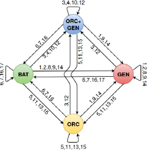
To describe the implemented control strategy, a state graph formalism is applied: each state corresponds to a particular combination of ON/OFF status of the different components, and some conditions are established for the transition from one state to the other. A state can vary from a timestep to the next one if the conditional statements differ. However, it should be remarked that PV, which produces power depending on the sun and not because it is started-up/shut-down, is not explicitly represented among system states. The following explanation clarifies this statement. The system state graph is presented in Fig. 6. All possible transitions have been indicated by arrows. Each number on the arrows refers to a particular condition (described below), which must be satisfied for a state transition in that direction (if at least one of the conditions at an arrow is satisfied, the transition occurs). Four states are distinguished in the system:
ORC: Only the ORC is running. This implies there is CSP-TES in the system.
GEN: Only the generator is in operation. Two configurations are possible: (a) either there is no ORC in the system or (b) there is an ORC and CSP but TES is discharged below the minimum temperature required for ORC operation.
ORC + GEN: Both ORC and generator are running. Two cases are possible: (a) there is no CSP, ORC is running with WHR from generator; (b) there is CSP and adequate charge in TES but ORC power output and battery SOC are insufficient to meet demand, invoking generator operation.
BAT: Neither of the ORC or the backup generator are running. Residual load is supplied by the batteries or else there is no residual load.
Fig. 6. State graph of the control strategy
The control strategy accounts for all possibilities, which have been synthesised in 17 conditions. These change-of-state conditions to be satisfied are the following, explained in Fig. 7. It is worthwhile to note that all of the above conditions depend on the Residual Load (RL) variable. This variable is defined as the load minus the PV generation (2):
7 Electrical dri ven c ont ro l
There is residual load: PV is not providing the entirety of the demand O
R C G E N R L > 0
Case 1: there is no battery bank
E b at = 0 There is no ORC 2 There is an ORC There is CSP
TES charge is too low to run the ORC 1
TES charge is adequate and RL > PORC 3
TES charge is adequate and RL ≤ PORC 5
There is no CSP 4
Case 2: there is a battery bank
E
b
at
> 0
Battery charge is adequate or full and its dischargeable power covers the RL 7
Battery charge is low or empty There is no ORC 8 There is an ORC There is CSP
TES charge is too low to run the ORC 9 PCSP > 0
(sunny) and TES charge is
adequate or full
Dischargeable power from
batteries covers RL- PORC 11
Dischargeable power from
batteries does not cover RL- PORC 12
PCSP = 0 (not sunny) and TES charge is
full
Dischargeable power from
batteries covers RL- PORC 13
Dischargeable power from
batteries does not cover RL- PORC 14
There is no CSP 10
There is no residual load: PV is covering the demand and producing in excess
R
L < 0
Case 1: there is no battery bank 6
Case 2: there is a battery bank
E b at > 0 Battery charge is not full There is an ORC
PV is not charging the batteries to its maximum capacity
and TES charge is adequate 15
PV is charging the batteries to its maximum capacity 16
TES charge is not adequate 16
There is no ORC 17
Battery charge is full 16
Fig. 7. Electricity driven rule-based control
As shown in Fig. 6, there is not a specific state for the PV installation. It is assumed that it is always ON, and the decision variable is the residual load: if positive, the model should to start-up some devices or use batteries to supply it. The dispatch is thus solely based on the presence or absence of residual load: as an example, the model takes the same decision for a night with no PV output and a 30kW demand as for a day with 20kW output of PV and a 50kW demand. This explains why the system states can be defined independently from PV.
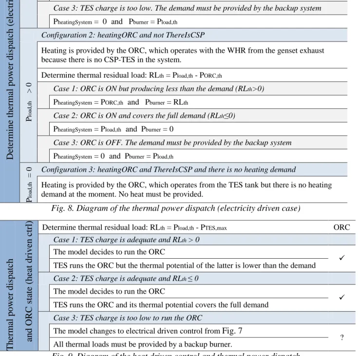
CHP systems can be electricity-driven (the unit supplies the electrical load and heat is a by-product) or heat driven (the unit supplies the heat demand and the power is a by-product). The same distinction is performed for the control of the ORC unit: it is electricity-driven when one of the three system configurations in Fig. 8 is present. In this case, the model runs the rule-based control
8
described in Fig. 7 to determine the electrical power dispatch, and right after, the model proposed in Fig. 8 to determine the dispatch of the thermal power.
Determine t hermal p o wer dispatc h (electric it y driven cas e) Configuration 1: heatingTES P lo ad ,t h ≥ 0
Heating is provided directly by the TES tank. The ORC therefore only starts if there is demand for electricity and if there is sufficient heat source availability.
Determine thermal residual load: RLth = Pload,th - PTES,max
Case 1: TES charge is adequate but not sufficient (RLth>0)
PheatingSystem = PTES,max and Pburner = RLth
Case 2: TES charge is adequate and covers the full demand (RLth≤0)
PheatingSystem = Pload,th and Pburner = 0
Case 3: TES charge is too low. The demand must be provided by the backup system PheatingSystem = 0 and Pburner = Pload,th
Configuration 2: heatingORC and not ThereIsCSP
P lo ad ,t h > 0
Heating is provided by the ORC, which operates with the WHR from the genset exhaust because there is no CSP-TES in the system.
Determine thermal residual load: RLth = Pload,th - PORC,th
Case 1: ORC is ON but producing less than the demand (RLth>0)
PheatingSystem = PORC,th and Pburner = RLth
Case 2: ORC is ON and covers the full demand (RLth≤0)
PheatingSystem = Pload,th and Pburner = 0
Case 3: ORC is OFF. The demand must be provided by the backup system PheatingSystem = 0 and Pburner = Pload,th
P lo ad ,t h
= 0 Configuration 3: heatingORC and ThereIsCSP and there is no heating demand
Heating is provided by the ORC, which operates from the TES tank but there is no heating demand at the moment. No heat must be provided.
Fig. 8. Diagram of the thermal power dispatch (electricity driven case)
T hermal po wer dis patc h and ORC state (hea t dri ven ctrl)
Determine thermal residual load: RLth = Pload,th - PTES,max ORC
Case 1: TES charge is adequate and RLth > 0
The model decides to run the ORC
TES runs the ORC but the thermal potential of the latter is lower than the demand
Case 2: TES charge is adequate and RLth ≤ 0
The model decides to run the ORC
TES runs the ORC and its thermal potential covers the full demand
Case 3: TES charge is too low to run the ORC
The model changes to electrical driven control from Fig. 7
? All thermal loads must be provided by a backup burner.
Fig. 9. Diagram of the heat driven control and thermal power dispatch
If heating is provided by the ORC and there is CSP-TES in the system, unless there is no heating demand (Configuration 3 in Fig. 8), the control should be heat driven. That is, the system must
9
decide to run the ORC if there is thermal demand, so that the latter is supplied by the ORC condenser and not by a more costly backup system.
Therefore, the heat-driven control provided in Fig. 9 defines the ORC state (ON/OFF). If the model decides to run the ORC, the following control consists in checking whether there is residual electrical load remaining, and if so, using the generator to provide it.
On the contrary, if the heat-driven control decides not to run ORC, the following step is to run an electricity-driven control (as stated in Case 3 in Fig. 9). This means, even if thermal demand production does not indicate ORC operation, it may occur that electrical demand provides the need. The total fuel consumption is related to the backup generator and the burner. The burner is assumed to work with a 84% of efficiency on the LHV, even for part-load operation. The LHV of the fuel is 46·103 kJ/kg.
6. Economic model
The micro-grid is based on a fee for service (i.e. prepaid smart meter) business model with positive cash flow and returns to debt capital for the power producer, which can be either the government or the private sector [2]. Moreover, the level of service at the household connections must be comparable to similar communities that are being served by the grid.
The economic model accounts for initial capital (CSP, LPG, PV and batteries), maintenance and operation costs (fuel consumption from the genset and burner), as well as for replacement cost of each component (in particular the batteries). Transmission and distribution lines, smart metering devices and ICT solutions for money transaction are also accounted for in the calculation of the tariff [2]. All economic inputs related to the project, the community of interest and the cost functions components are presented and described in [1] (section 5.8). With the maintenance, operating and investment costs defined, the Levelized Cost Of Electricity can be computed according to the following:
∑ ( ) ∑ ( ) (3) Because thermal demand is also supplied by the micro-grid, a Levelized Cost Of Energy (electrical+thermal) is computed to take into account both electrical and thermal loads. Equation (3) is used, with the burner now taken into account in both operating Oy and investment Iy costs, and
the thermal load added to the annual load Ey.
7. Sizing optimization
The first step towards the design of a viable energy system is to technically specify and size a combination of different power sources. However, the system must also be economically feasible. Thus, the optimum configuration of the system should be determined based on a financial analysis (e.g. minimizing Levelized Cost of Energy (LCOE), maximizing Internal Rate of Return (IRR), etc.). Therefore, a cash flow model is coupled to the technical-dispatching model. The main goal of the design optimization is to find the system infrastructure and the optimum power flow control strategy that achieves the minimum levelized cost of energy (USD/kWh) to consumers. The tariff is based on cost recovery of the capital and operating costs.
The problem is a non-linear optimization problem without integer variables. At each evaluation, the solver must simulate a full year of operation, compute all the yearly energy flow, and deduce the levelized cost of energy (LCOE), which is the variable to be optimized.
There are several types of optimization techniques that can be used to determine the optimum solution of a complex (non-necessarily convex) non-linear problem. Based on the study performed in [3], PSO is selected as the algorithm to run the microgrid optimization.
10
The optimization results that size the described microgrid system are evaluated in section 7.1. However, two other simulations are also performed to evaluate the size of the system if other costs were presented or other possible configurations were offered to the model.
7.1. Optimization 1: Optimal sizing
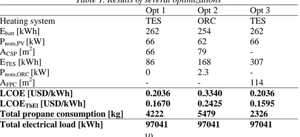
The obtained sizing results are presented in Table 1. Interestingly, the model only chooses to install PV and batteries to provide the electrical load. Moreover, the optimization shows that it is economically preferable not to install an ORC and produce the thermal load with the backup burner mostly, but also with CSP-TES.
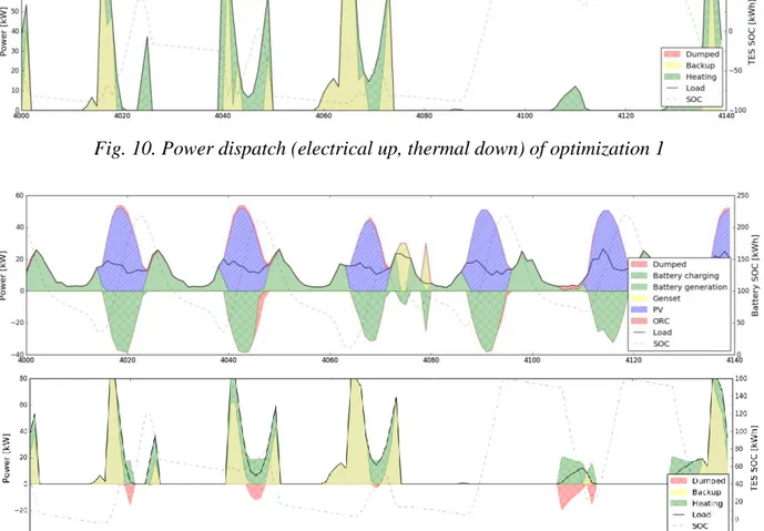
Fig. 10 shows part of the power dispatch in May. The electrical peak load usually occurs in the mornings and the evenings, with the lowest values during the night. The optimum size of PV panels does not only provide the load during daylight but also charges the batteries at its maximum (batteries SOC is indicated at the right axis). Therefore, it is almost ensured that the batteries provide the entire load during the night and the backup generator is almost never used. However, in some days when the irradiation is lower (3rd blue peak in Fig. 10), the batteries cannot supply the entire load and the generator is turned on.
7.2. Optimization 2: Modified investment costs
The model decision is highly influenced by the costs relative to each subcomponent. In the current economic inputs, PV and batteries are more cost-effective than the ORC. The main goal of this optimization is thus to see if the model would invest in ORC capacity with more favorable investment costs. The price of PV and batteries is increased, while the price of the ORC is decreased. The CSP and TES prices are kept unchanged. The new prices used in this optimization are presented in Table 2, together with the original ones for the sake of comparison.
The obtained results are shown in Table 1. Differently than in Optimization 1, the simulation chooses to install an ORC, CSP and TES. However, even with the proposed decrease in ORC cost, the optimum system still relies mostly on PV power generation and battery storage. The optimal ORC power is 2.3kW, and as it can be seen in Fig. 11, it does not influence much the power dispatch.
7.3. Optimization 3: Considering flat plate thermal collectors
At the light of the results of the optimal sizing, the use of flat plate solar thermal collectors is evaluated. In the case of heat supply only, this technology is indeed more cost-effective than CSP and could therefore mitigate the use of the burner.
The obtained results are presented in Table 1. As expected, the levelized cost of energy is lower since the optimal sizing generates more heat through renewable sources than in optimization 1. The dispatch of thermal power is shown in Fig. 12. This would thus be the optimal solution for the studied community.
Table 1. Results of several optimizations
Opt 1 Opt 2 Opt 3
Heating system TES ORC TES
Ebatt [kWh] 262 254 262 Pnom,PV [kW] 66 62 66 ACSP [m2] 66 79 - ETES [kWh] 86 168 307 Pnom,ORC [kW] 0 2.3 - AFPC [m2] - - 114 LCOE [USD/kWh] 0.2036 0.3340 0.2036 LCOEThEl [USD/kWh] 0.1670 0.2425 0.1595
Total propane consumption [kg] 4222 5479 2326
11
Total PV generation [kWh] 125469 117865 125469
Total ORC generation [kWh] 0 1694 0
Total genset generation [kWh] 2040 2940 2040
Total thermal load [kWh] 58745 58745 58745
Total heating system generation [kWh] 22930 17061 42791
Total burner generation [kWh] 35815 45277 15954
Table 2. Investments costs for optimization 2
Parameter Previous value New value Units
cbatt 130 300 USD/kWh
cpanels 1000 1500 USD/kW
cORC 2000 1000 USD/kW
Fig. 10. Power dispatch (electrical up, thermal down) of optimization 1
12
Fig. 12. Thermal power dispatch of optimization 3
12. Conclusions
Starting from the generator’s models (PV, ORC and LPG genset), the storage unit’s models (batteries and TES) and the electricity and heating demand profiles, a microgrid model is built by interconnecting all of its subcomponents. Most of the micro-grid related literature focuses on electrical power only. In this work, a special focus has been paid to the co-optimization of both the thermal and electrical load satisfaction since it can improve the overall energy efficiency of the system. The most relevant part of this work is thus the proposed rule-based control strategy, which accounts for interactions between thermal and electrical loads. The control dispatches heat and power flows of each component in order to cover the demand while minimizing the fuel consumption. The developed microgrid model together with an economical model is finally wrapped into a non-linear optimization run by the PSO algorithm.
For Ha Nkau, the studied community in Lesotho, the determined optimal system infrastructure is composed of only PV (66 kW) and batteries (262 kWh), and the optimum control strategy achieves an electrical tariff (LCOE) value of 0.203 USD/kWh. Fuel consumption is mainly generated by the burner, which supplies most of the thermal load together with CSP (66 m2) and TES (86 kWh). The tariff accounting for electrical and thermal loads is 0.167 USD/kWh. The project presents an investment cost of 154425 USD and a life-time of 15 years. Batteries are replaced every 8 years. The obtained tariff is considered to be an affordable cost for householders and institutions (health clinics and schools) of a community. Moreover, the low propane consumption of 4221 kg per year dramatically reduces CO2 emissions compared to a genset-only configuration, which was also a
goal of this work.
Because of the high solar potential of Lesotho, the possibility of installing flat-plate solar thermal collectors together with the adequate TES tank is also be evaluated. The results show that his cost-effective technology mitigates the use of the burner. Therefore, it not only reduces CO2 emissions
but also provides a lower levelized cost of energy (0.159 USD/kWh).
The model is designed to cover demand at all times. Although the optimal solution found by the proposed rule-based control strategy may be less optimal than if a perfect foresight control was used, the obtained power flows are more realistic since they account for the inefficiencies encountered in real systems. The same model can be used when only electricity is supplied to a community.
Finally, the microgrid simulation results show that although having assets such as co-generation and dispatchability, the ORC is more expensive than PV and the batteries storage. This is partly explained by the fact that the heat load of a clinic and a school remain limited: heat production is more cost-effective with a burner than installing a micro-CSP plant with ORC. Another possibility is to include the use of locally harvested biomass as a thermal source to supplement solar thermal collection, which could raise the capacity factor of the ORC and improve the value of investment. It should finally be noted that the presented rule-based control is a first attempt to propose a thermal-electricity interactive control. The code can be used to evaluate a number of different simulations, the results of which could serve to improve the rule based control. Such improvements could lead to a better use of the ORC and of the thermal storage, which could increase their economic viability.
13
Acknowledgments
This work was carried out in close collaboration with STG International. This support is gratefully acknowledged.
References
[1] Q. Altés Buch, “Mechanical design, control and optimization of a hybrid solar microgrid for rural electrification and heat supply in sub-Saharan Africa,” Master Thesis, University of Liege, Belgium, 2016.
[2] M. S. Orosz and A. V. Mueller, “Dynamic Simulation of Performance and Cost of Hybrid PV-CSP-LPG Generator Micro Grids With Applications to Remote Communities in Developing Countries,” Jun. 2015.
[3] S. Ghaem Sigarchian, M. S. Orosz, H. F. Hemond, and A. Malmquist, “Optimum design of a hybrid PV–CSP–LPG microgrid with Particle Swarm Optimization technique,” Appl. Therm. Eng., 2016.
[4] K. Emery, “Measurement and Characterization of Solar Cells and Modules,” in Handbook of Photovoltaic Science and Engineering, A. Luque and S. Hegedus, Eds. John Wiley & Sons, Ltd, 2010, pp. 797–840.
[5] S. Quoilin, M. Orosz, H. Hemond, and V. Lemort, “Performance and design optimization of a low-cost solar organic Rankine cycle for remote power generation,” Sol. Energy, May 2011. [6] O. Cummins, RV generator set Quiet Gasoline TM Series RV QG 4000. 2016.