EXTENDING α-EXPANSION TO A LARGER SET OF REGULARIZATION FUNCTIONS
Mathias Paget, Jean-Philippe Tarel
∗Lepsis/Cosys, IFSTTAR,
14-20 Boulevard Newton,
F-77420 Champs-sur-Marne,
Universit´e Paris-Est, France
Laurent Caraffa
Matis, IGN,
73 Avenue de Paris,
F-94165 Saint-Mand´e, France
ABSTRACT
Many problems of image processing lead to the minimization of an energy, which is a function of one or several given im-ages, with respect to a binary or multi-label image. When this energy is made of unary data terms and of pairwise regular-ization terms, and when the pairwise regularregular-ization term is a metric, the multi-label energy can be minimized quite rapidly, using the so-calledα-expansion algorithm. α-expansion con-sists in decomposing the multi-label optimization into a series of binary sub-problems called move. Depending on the cho-sen decomposition, a different condition on the regularization term applies. The metric condition forα-expansion move is rather restrictive. In many cases, the statistical model of the problem leads to an energy which is not a metric. Based on the enlightening article [1], we derive another condition for β-jump move. Finally, we propose an alternated scheme which can be used even if the energy fulfills neither theα-expansion nor β-jump condition. The proposed scheme applies to a much larger class of regularization functions, compared to α-expansion. This opens many possibilities of improvements on diverse image processing problems. We illustrate the advan-tages of the proposed optimization scheme on the image noise reduction problem.
Index Terms— Minimization, Discrete optimization, Regularization, Markov Random Field,α-expansion, Graph-cuts, Denoising,Noise reduction.
1. INTRODUCTION
Image processing problems are usually set as the minimiza-tion of an energy with respect to the unknown variables of the problem. The Bayesian approach provides ways to derive the energy of the problem from its statistical model. This energy is a function of the observations and of the unknown variables which are both numerous. In image processing, the used sta-tistical models are generally Markov Random Fields. If sev-eral optimization methods for large problems are available, each method has its own field of application due to restrictive
∗Thanks to FUI AWARE project for funding.
conditions of use on the energy. Matching between the energy derived from the Bayesian approach and the conditions of use of the optimization method is often tricky.
α-expansion is a discrete multi-label optimization method, introduced by [2, 3], where successive binary sub-problems are solved. The sub-problem, which is parametrized byα, consists in deciding for every pixels if setting the current pixel label to α allows to decrease the total energy. When the energy of the sub-problem is sub-modular, the binary sub-problem can be minimized to a global minimum. Never-theless theα-expansion algorithm only converges towards a local minimum of the energy w.r.tα-expansion move space, as a succession of decreasing steps of the energy.α-expansion is well known as one of the fastest algorithm to optimize an energy on a graph, with unary data terms and pairwise regu-larization data terms. However, the condition on the energy forα-expansion to be applied, is that the regularization term must be a metric. Examples of metric pairwise terms are con-cave functions of the absolute difference of the two labels.
This condition is rather restrictive. For instance, α-expansion can not cope with the standard Gaussian prior. Indeed, when a Gaussian pairwise prior is used, the regular-ization term is a quadratic function of the difference of the two labels. When the pairwise term is a concave continuous function of the absolute difference of two labels, this implies that the regularization function is not smooth when the two labels are equals. This is an important limitation, since due to the presence of Gaussian noise or slow variations, it is useful to have a locally quadratic shape at the zero of the function which applies to the two labels difference. As pointed in [3], this property is also important in disparity reconstruction from stereo images of thin objects without filling the hole between them.
Our objective is thus to find ways to extendα-expansion to a larger set of energies. In Sec. 2, from the enlightening theory summarized in [1], a simple implementation of the α-expansion algorithm is obtained and the condition the regu-larization term must fulfill is again derived. Then, the same kind of derivation is performed, for a different case, where the sub-problem is now aβ-jump. A sufficient condition of use
is that the pairwise regularization term is a convex function of the label difference. Then, we propose in Sec. 3, a scheme to optimize an energy where the pairwise regularization term is neither a concave nor a convex function of the label differ-ence. In Sec. 4, we illustrate the advantage of the proposed optimization scheme on the image noise reduction problem.
2. MULTI-LABEL MINIMIZATION
We consider the following energyE(l) to be minimized with respect to the label imagel:
E =X u∈I g(lu) + X (u,v)∈N f (lu, lv), (1)
whereI is the set of sites in the image, N is the set of neigh-borhood links,u and v are sites, f is the pairwise regulariza-tion funcregulariza-tion andg is the unary data cost function. We assume that functionf is non-negative. ludenotes the label at the site
u. Labels are assumed in a set L of ordered labels.
Let us recall that the global minimum of such discrete en-ergy can be obtained, when the functionf is convex, as shown in [4], using graph-cuts. However, this algorithm requires many computations. In practice, approximate solutions, such as [2], are usually preferred. In this latter approach, the ini-tial multi-label problem is decomposed into successive binary sub-problems, which are solved using graph-cuts. The binary sub-problem consists in choosing or not a new label for each site, given a rule. This is called a move. A set of moves which spans the label entire set is named a move space. Different rules and thus different move spaces were proposed such as: α-expansion, jump, swap, relabeling [3]. The set of regular-ization terms which can be used in the energy is different for each type of move.
In [1], it was proposed to use the Quadratic Pseudo Boolean Optimization (QPBO) theory to rewrite binary sub-problems using a pseudo-Boolean function. When the ob-tained quadratic pseudo-Boolean function is sub-modular, i. e. coefficients before quadratic terms are all negative, a graph can be built and the sub-problem can be minimized as a maximum flow optimization on the associated graph [5]. As a consequence, the QPBO theory gives us a way to derive the condition the pairwise regularization term must fulfill to be used with a given type of move spaces.
Let lu be the current label at site u, and ˆlu the newly
proposed label at this site. The sub-modularity of the binary problem implies, for the all pairs of sites(u, v) ∈ N :
f (lu, lv) + f ( ˆlu, ˆlv) ≤ f (lu, ˆlv) + f ( ˆlu, lv), (2)
Notice that this inequality is fulfilled whenlu = ˆluor when
lv = ˆlv. We now focus on two kinds of moves:α-expansion
andβ-jump moves.
2.1. α-expansion
Anα-expansion move consists in proposing a label α for ev-ery siteu, where α is given. This move can be formally writ-ten as ˆlu = α, ∀u ∈ I. In such a case, the condition of
sub-modularity (2) becomes:
f (lu, lv) + f (α, α) ≤ f (lu, α) + f (α, lv) (3)
Iff (x, x) is a constant k, for all u, the previous condition is fulfilled when the functionf (x, y) − k is a metric. We now consider a useful particular case, wheref (lu, lv) is assumed
to be a functionf∗
of the label difference, i.e, f (lu, lv) =
f∗(l
u−lv), then the condition is :
f∗
(x + y) + f∗
(0) ≤ f∗
(x) + f∗
(y), (4)
for allx, y ∈ R2. This means thath(x) = f∗(x) − f∗(0)
is sub-additive on R. A sufficient condition for h(x) to be sub-additive is to be even and concave on R+. Such func-tions can not be smooth in zero. As a consequence,f∗
is not smooth on R. This is an important limitation in the usage of α-expansion, since we are interested in using a smooth func-tion for the pairwise regularizafunc-tion term.
In summary, a first sufficient condition of use of the α-expansion is that the pair-wise regularization term is a metric. A second sufficient condition is that it is an increasing con-cave function of the label absolute difference. Following [1], it is not difficult to derive the graph where max flow should be applied to obtain the solution of eachα-expansion binary sub-problem.
2.2. β-jump move
Aβ-jump move consists in proposing an increment or decre-ments of the current labels by valueβ, for every site u. For-mally, ˆlu = lu+ β, ∀u ∈ I. For a β-jump, the condition of
sub-modularity (2) becomes:
f (lu, lv) + f (lu+ β, lv+ β) ≤ f (lu, lv+ β) + f (lu+ β, lv).
(5) Like in the previous section, we now consider the particular case, wheref (lu, lv) is assumed to be a function f∗ of the
label difference. The previous inequality can be rewritten as: 2f∗
(x) ≤ f∗
(x + β) + f∗
(x − β), (6)
for allx, β. After substitution of x = (y + z)/2 and β = (y − z)/2, we deduce that f∗ is mid-convex: f∗ (y + z 2 ) ≤ f∗(y) + f∗(z) 2 , (7)
From Bernstein-Doetsch theorem,f∗
being also upper bounded, f∗(x) is a convex function on the label interval.
In summary, considering pair-wise regularization with the label difference, a sufficient and necessary condition of use of
theβ-jump is that the pair-wise regularization term is convex. Following [1], it is also not difficult to derive the graph where max flow should be applied to obtain the solution of each β-jump binary sub-problem.
2.3. Extended Smooth Exponential Family
Given a problem, the choice of the energy can be interpreted, in the Bayesian approach, as the implicit choice of a statistical model of the problem. As explained in [6, 7], a useful fam-ily of probability distribution functions (pdf) named Smooth Exponential Family (SEF) can be used to help in the statis-tical modeling. The advantage of the SEF family is that it is parameterized by only two parameters: the shape parame-tera and the scale parameter s. To better fit observed data, we proposed an Extended SEF family (ESEF) where an ex-tra parameterk is added. The ESEF pdf is defined, up to a normalization factor, asexp(−ESEF (b)) where:
ESEF (b) = k a((1 + b2 2s2) a−1). (8) All functions in the ESEF family are smooth and several well known distributions can be found for particular values ofa, for instance: Gaussian pdf fora = 1, smooth Laplace pdf for a = 0.5, Cauchy and T pdfs as a limit case when a goes towards0, Geman&Maclure pdf for a = −1. Using the Bayesian approach, it is the minus of the log of the pdf which appears in the energy, i.eESEF (b) defined in (8).
The behavior of the ESEF function around zero is al-ways quadratic. Therefore, α-expansion can not be used. When theESEF function is convex, i.e when a ≥ 0.5, the β-jump can be used, but not in the other cases. Another exam-ple of useful regularization function which can not be used, neither with α-expansion nor with β-jump, is the truncated quadratic function.
3. PROPOSED APPROACH
To be able to cope with a large set of pairwise regulariza-tion terms, we propose an alternated scheme between an α-expansion move space and aβ-jump move space. Since the condition of use of each decreasing energy algorithm is not always fulfilled, the optimization is limited to sites where the problem is sub-modular.
For a site where the sub-modularity condition (2) is veri-fied for all its links, a new label is proposed. But, when this condition is not fulfilled, the same label as the current label is proposed. As a consequence, during anα-expansion move or aβ-jump move, only the sites where the sub-modularity condition is verified can be modified. We call this variant as partial. This means that, if the energy is decreased at each step, the energy will not necessarily converge to a local mini-mum due to the possibility of sites with a fixed label. The ad-vantage of alternating between partialα-expansion and partial
Algorithm 1AlternatedOptimization Initialize labels E0←ComputeEnergy whileEnergyIsStrictlyDecreasing do forα ∈ L do P artialAlphaExpansion(α) forβ ∈ L do P artialBetaJump(β) P artialBetaJump(−β) Algorithm 2P artialAlphaExpansion(α) fori ∈ I do f lagi ←AllLinksSubmodular fori ∈ I do iff lagithen ˆ li←α else ˆ li←li DoGraphCut Algorithm 3P artialBetaJump(β) fori ∈ I do f lagi ←AllLinksSubmodular fori ∈ I do
iff lagi& (li+ β) ∈ L then
ˆ li←li+ β else ˆ li←li DoGraphCut
β-jump moves is to try to minimize the number of sites with a fixed label due to the difference in their conditions of use. The alternated optimization is stopped when neitherα-expansion norβ-jump move spaces strictly decrease the energy.
The proposed scheme is shown in Algo. 1, with the partial α-expansion in Algo. 2 and the partial β-jump in Algo. 3. No-tice that sinceα-expansion and β-jump moves are performed on the same graph structure, every graph-cut steps only need to update the graph values and not to rebuild the graph.
4. IMAGE NOISE REDUCTION
We test the proposed schemes on the image noise reduction problem. On each image, we compute the intensity differ-ence histogram over all neighbors. A ESEF model is fitted on the observed distribution to estimatef , using Maximum Likelihood (ML) criterion. Then a Gaussian noise (with std 10) is added to the images, so g is set as -log of this pdf, i.e a square function.
4.1. Fixed sites
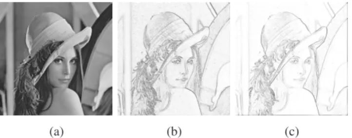
Fig. 1(a) shows the ”Lena” image. The used regularization function is a ESEF function witha = 0.4, s = 10 and k = 1.
(a) (b) (c)
Fig. 1: (a) Lena image, (b) in gray, pixels where intensity value may be fixed duringα-expansion (multiplied by 4), (c) fixed pixels duringβ-jump (multiplied by 2).
This function is locally convex around zero and concave for higher values. In Fig. 1(b), the number of fixed labels during theα-expansion move is shown, with α ∈ L. Fig. 1(c) shows theβ-jump case. We remark that fixed pixels are mainly along objects edges in both cases. This can be explained by the con-cave part of the ESEF function whenβ-jump is used. When α-expansion is used, fixed pixels only occur when the value ofα is between the two neighbor label values. This case is thus more likely to happen at edges. Notice that on the edges, the numbers of fixed labels duringα-expansion are lower than forβ-jump in our experiments.
4.2. Optimization scheme comparison
A pairwiseL1regularization is used in order to compare
per-formances ofα-expansion, β-jump and alternated scheme on the same energy. Indeed,L1regularization fulfills both
condi-tions (3) and (5), and thus there is no pixel with a fixed label. Over 7 tested images, the 3 optimization schemes give the same final energy. This illustrates the consistancy between the different schemes.
4.3. Image noise reduction comparison
The comparison of the previous different methods with bilat-eral filter, in term of Peak Signal-to-Noise Ratios (PSNR), af-ter parameaf-ter optimization, leads to quite similar PSNR. Nev-ertheless, obtained results differ in terms of smoothness. For instance, Fig. 2 presents details obtained from ”Cameraman” and ”Lena” images usingα-expansion (first column) and al-ternated scheme (second column). In the two first lines, the regularization term for the alternated scheme comes from the ESEF pdf fitting. To applyα-expansion, the previous ESEF pdf is approximated by the closest concave function on R+. In the third line, aL1regularization is used withα-expansion
(left), and a smoothedL1 (ESEFa = 0.5, s = 3, k = 1)
function with the alternated scheme. One can notice the dif-ferences in areas of slow intensity variation, such as the sky in ”Cameraman” or Lena’s cheek. α-expansion leads to a staircase effect due to the concave regularization. Results are smoother with alternated scheme, thanks to a regulariza-tion funcregulariza-tion which is locally convex around zero, even if the noise is a little less decreased in flat areas. On seven images,
Fig. 2: Noise reduction obtained withα-expansion (fist col-umn) and Alternated scheme (second colcol-umn), on line 1 and 2 for approximated ESEF and ESEF model, on line 3 forL1
and Smoothed-L1model.
alternated scheme is slower by a factor between1.1 to 2.5, compared toα-expansion.
5. CONCLUSION
From [1], we derive again that concave functions of the ab-solute labels difference can be used withα-expansion and we obtain that convex functions can be used withβ-jump. This leads us to the idea to alternated betweenα-expansion and β-jump to minimize an energy where regularization function is neither concave nor convex. The proposed optimization scheme can be applied to a set of energies which is much larger that the usable set forα-expansion. We illustrated the advantages of the proposed scheme for image noise reduction. This opens many possibilities of improvements on diverse im-age processing problems.
6. REFERENCES
[1] Endre Boros and Peter L Hammer, “Pseudo-boolean op-timization,” Discrete applied mathematics, vol. 123, no. 1, pp. 155–225, 2002.
[2] Yuri Boykov, Olga Veksler, and Ramin Zabih, “Fast ap-proximate energy minimization via graph cuts,” Pattern Analysis and Machine Intelligence, IEEE Transactions on, vol. 23, no. 11, pp. 1222–1239, 2001.
[3] Olga Veksler, Efficient graph-based energy minimization methods in computer vision, Ph.D. thesis, Cornell Uni-versity, 1999.
[4] Hiroshi Ishikawa, “Exact optimization for markov ran-dom fields with convex priors,” Pattern Analysis and Ma-chine Intelligence, IEEE Transactions on, vol. 25, no. 10, pp. 1333–1336, 2003.
[5] Vladimir Kolmogorov and Ramin Zabin, “What energy functions can be minimized via graph cuts?,” Pattern Analysis and Machine Intelligence, IEEE Transactions on, vol. 26, no. 2, pp. 147–159, 2004.
[6] Sio-Song Ieng, Jean-Philippe Tarel, and Pierre Charbon-nier, “Modeling non-gaussian noise for robust image analysis,” in Proceedings of International Conference on Computer Vision Theory and Applications (VISAPP’07), Barcelona, Spain, 2007, pp. 183–190.
[7] Laurent Caraffa, Jean-Philippe Tarel, and Pierre Char-bonnier, “The guided bilateral filter: When the joint/cross bilateral filter becomes robust,” IEEE Transactions on Image Processing, vol. 24, no. 4, pp. 1199–1208, Apr. 2015.