Science Arts & Métiers (SAM)
is an open access repository that collects the work of Arts et Métiers Institute of Technology researchers and makes it freely available over the web where possible.
This is an author-deposited version published in: https://sam.ensam.eu
Handle ID: .http://hdl.handle.net/10985/20275
To cite this version :
Atal Anil KUMAR, Jeau-Francois ANTOINE, Gabriel ABBA - Input-Output Feedback Linearization for the Control of a 4 Cable-Driven Parallel Robot - 9th IFAC Conference MIM 2019 - Vol. 52, n°13, p.707-712 - 2019
Atal Anil Kumar* Jean-François Antoine*
Gabriel Abba*
* Arts et Métiers ParisTech, Université de Lorraine, LCFC, F-57000 Metz, France
(e-mails: [email protected], [email protected], [email protected])
Abstract: This paper presents the control of an under-constrained 4 Cable-Driven Parallel Robot (CDPR) using input-output feedback linearization technique. The dynamic model of the CDPR is first formulated by taking into account the Euler angle rates. Following this the input-output feedback linearization method is implemented to decouple the output and input. A linear feedback controller is then designed using pole placement method to control the CDPR. The control law is then verified by simulation using MATLAB software. Simple trajectories are then tested with and without the presence of noise to analyze the behavior of the control law.
Keywords: Under-constrained CDPR, Input-output decoupling, Euler angle rates, pole-placement
technique, feedback linearization.
1. INTRODUCTION
Cable-Driven Parallel Robots (CDPRs) are a special variant of traditional parallel robots in which the traditional rigid links are replaced by flexible cables to connect the movable end-effector and the fixed base. The position and orientation of the moving platform are controlled by the coordinated retraction and extension of the cables which are driven by winch consisting of a tensioning motor and spool or a linear actuator moving a pulley system (Merlet and Daney, 2010). Some of the first ideas on CDPRs were presented in the late 1980s and 1990s by Landsberger (Landsberger, 1985), Higuchi et al. (Higuchi, 1988), and Albus et al. (Albus et al., 1993). CDPRs have a number of advantages when compared to the traditional serial-link and other parallel type robots in terms of large load capacity, low inertia, high energy efficiency, large workspace and so on. In addition to these, they also are easily reconfigurable, less expensive to construct, easy to transport, assemble and disassemble etc.(Gosselin, 2014). However, one of the important challenges in the design of the CDPRs arises from the fact that cables can only pull and not push. As a result of this a unilateral constraint exists in which the cables must always be maintained in tension. Because of this constraint, CDPRs in general need a larger number of cables than the number of degrees of freedom (dof) to fully restrain or control the moving platform (Ming, 1994).
CDPRs are mainly classified as over-constrained, fully-constrained and under-fully-constrained (Verhoeven, 2004). A CDPR with m-cables and n-dof is said to be fully-constrained if it has one cable more than the number of degrees of freedom, i.e. m=n+1. In such a type of CDPR, all degrees of freedom can be controlled through the cables. An over-constrained CDPR has the condition m≥n+1. An under-constrained CDPR is one in which the number of cables is less than or equal to the number of degrees of freedom i.e. m≤n. Such CDPRs have
at most one feasible solution for cable tensions and mostly rely on gravity for keeping the cables taut. CDPRs with a limited number of cables are used in several applications in which the task to be performed requires a limited number of controlled freedoms or a limitation of dexterity is acceptable in order to decrease complexity, cost, set-up time, likelihood of cable interference etc. (Abbasnejad and Carricato, 2015).
Control of CDPRs has received a lot of interests from a number of researchers. Several approaches have been used by the research community for the control of CDPRs namely Lyapunov based control (Alp and Agrawal, 2002), sliding mode (Oh and Agrawal, 2006), fuzzy plus PI control (Zi et al., 2008) and so on. However, very few works are available on the control of under-constrained CDPMs. Some of the approaches are dynamic trajectory planning (Gosselin et al., 2012), anti-sway trajectory generation based on input-shaping (Park et al., 2013), zero-vibration input shaping scheme (Hwang et al., 2016), flatness-based control (Maier and Woernle, 1999) and so on.
This paper deals with the control of an under-constrained 4 cable-driven spatial parallel robot. Since the number of cables (4) is less than the number of degrees of freedom of the platform (6), the platform has extra dofs in motion which could cause unwanted sway or oscillations, as a result of which, the controllable workspace of the platform is limited (Hwang et al., 2016). The calculation of the static equilibrium workspace for the CDPR is calculated by the authors in (Kumar et al., 2019). Following this, the dynamic model of the CDPR is formulated. Using the results obtained from the previous studies, a nonlinear control scheme is developed in this work using the input-output linearization technique. The simulation results indicate that this scheme can be applied for the control of the CDPR designed.
The paper is organized as follows: section 2 presents the dynamic model of the CDPR followed by section 3 which introduces the equations and the steps involved for the input output feedback linearization in general. The implementation of the control technique for the CDPR is presented in section 4 followed by the results in section 5. The conclusion and future work are presented in the last section of the paper.
2. DYNAMIC MODEL OF THE CDPR
The equations used in the modelling of CDPR is presented in this section. The modelling and analysis methods developed for conventional rigid link manipulators cannot be directly applied to the cable-driven robots because of the unilateral constraints where the tensions in the cables must be considered.
A general sketch of cable-driven parallel robot is shown in (Fig. 1).
Fig. 1: Simple sketch of one of the cables of the CDPR
A fixed reference frame (O, x, y, z) attached to the base of a CDPR is referred to as the base frame. A moving reference frame (P, x’, y’, z’) is attached to the mobile platform where P is the reference point of the platform to be positioned by the mechanism. From (fig. 1), ai and bi are respectively defined as
the vector connecting point O to point Ai and the vector
connecting point P of the platform to the point Bi, both vectors
being expressed in the base frame. The position p of the mobile platform is given by 𝑂𝑃⃗⃗⃗⃗⃗ .Certain assumptions are made to reduce the complexity of computation in the modelling procedure (Gosselin, 2014):
1) The mass of the cables is negligible and the cables are non-elastic.
2) The ith cable is assumed to be taut between points and is
therefore considered a straight segment and is denoted by 𝜌𝑖.
3) The moving platform is assumed to be a rigid body, defined by its mass and inertia matrix.
The equations of motion for a CDPR can be derived using Newton–Euler formulations provided all cables are in tension as shown in (1) (Diao and Ma, 2009).
[𝑚𝐼3×3 03×3 03×3 𝐼𝑃 ] [𝑝̈ 𝜔̇] + [ 03×1 𝜔 × 𝐼𝑃𝜔 ] + [−𝑚𝑔0 3×1] = 𝐽 𝑇𝜏 (1)
In this equation, m denotes the mass of the end-effector, IP is
a 3×3 matrix and denotes the inertia tensor of the end-effector about point P in the base frame, I3×3 is a 3×3 identity matrix, g
denotes the gravity acceleration vector, τ denotes the vector of cables forces while scalar ti denotes the tension force of the ith
cable, 𝜔 = [𝜔𝑥, 𝜔𝑦, 𝜔𝑧]𝑇 denotes the velocity vector of the
orientation, 𝑝 = [𝑝𝑥, 𝑝𝑦, 𝑝𝑧]𝑇 denotes the position vector.
Consider 𝑋 = [𝑥, 𝑦, 𝑧, 𝛼, 𝛽, 𝛾]𝑇
as generalized coordinates vector, in which 𝜃 = [𝛼, 𝛽, 𝛾]𝑇 denotes the vector of a set of
Euler angles. With this definition the rotation matrix can be written in terms of Euler angles as:
𝑅 = [
𝑐𝛽𝑐𝛾 𝑐𝛾𝑠𝛼𝑠𝛽 − 𝑐𝛼𝑠𝛾 𝑐𝛼𝑐𝛾𝑠𝛽 + 𝑠𝛼𝑠𝛾 𝑐𝛽𝑠𝛾 𝑐𝛼𝑐𝛾 + 𝑠𝛼𝑠𝛽𝑠𝛾 −𝑐𝛾𝑠𝛼 + 𝑐𝛼𝑠𝛽𝑠𝛾
−𝑠𝛽 𝑐𝛽𝑠𝛼 𝑐𝛼𝑐𝛽
] (2)
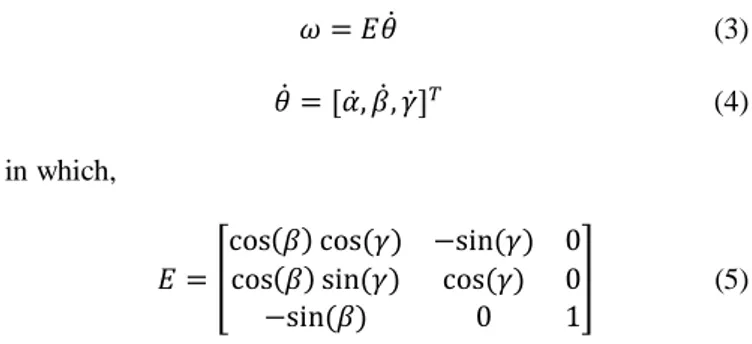
where, s and c represent sin and cos functions, respectively. The angular velocity of the end-effector can be written in the following form,
𝜔 = 𝐸𝜃̇ (3) 𝜃̇ = [𝛼̇, 𝛽̇, 𝛾̇]𝑇 (4)
in which,
𝐸 = [
cos(𝛽) cos (𝛾) −sin (𝛾) 0 cos(𝛽) sin (𝛾) cos (𝛾) 0 −sin (𝛽) 0 1
] (5)
The equations of motion can be written in terms of X using the notations defined above. By some manipulations these equations may be derived as,
𝑀(𝑋)𝑋̈ + 𝐶(𝑋, 𝑋)̇𝑋̇ + 𝐺(𝑋) = 𝐽𝑇𝜏 (6) where, 𝑀(𝑋) = [𝑚𝐼03×3 03×3 3×3 𝐼𝑃𝐸 ] 𝐶(𝑋, 𝑋)̇𝑋̇ = [ 03×3 𝐼𝑃𝐸̇𝜃̇ + (𝐸𝜃̇) × 𝐼𝑃(𝐸𝜃̇) ] 𝐶(𝑋, 𝑋̇) = [003×3 03×3 3×3 𝐼𝑃𝐸̇ + (𝐸𝜃̇)×(𝐼𝑃𝐸)] 𝐺(𝑋) = [−𝑚𝑔0 3×1]
in which, the matrix (𝐸𝜃̇)× is a skew-symmetric matrix
defined by the components of the angular velocity vector as
(𝐸𝜃̇)×= [
0 −𝜔𝑧 𝜔𝑦
𝜔𝑧 0 −𝜔𝑥
−𝜔𝑦 𝜔𝑥 0
] (7)
Equation (6) is finally represented as
where, 𝑁(𝑋, 𝑋)̇𝑋̇ = 𝐶(𝑋, 𝑋)̇𝑋̇ + 𝐺(𝑋)
Equation (8) is then used for the implementation of the input- output feedback linearization method.
3. INPUT-OUTPUT FEEDBACK LINEARIZATION The development of differential geometric approach in control theory for nonlinear systems has helped in solving many nonlinear control problems such as decoupling, output regulation, and tracking (Kim, 1991). In this approach, feedback linearization has been used extensively since a long time for SISO (Single-Input Single-Output) as well as MIMO (Multi-Input Multi-Output) nonlinear systems. Feedback linearization is conveniently divided into two categories; input-output linearization and exact state-space linearization. We confine ourselves to the first category as input-output linearization provides a basis for more sophisticated and complicated control schemes for a nonlinear system. This method transforms a certain class of nonlinear systems into linear system by a proper coordinate change and a linearizing state feedback. Further explanation of the technique in detail can be found in (Isidori, 2013).
The mathematical approach of the input-output feedback linearization method for a nonlinear MIMO dynamic system of nth order with m number of inputs and outputs is presented
here.
Consider a MIMO system described in the affine form as given below:
𝑥̇(𝑡) = 𝑓(𝑥, 𝑡) + 𝑔1(𝑥, 𝑡)𝑢1(𝑡) + ⋯ + 𝑔𝑚(𝑥, 𝑡)𝑢𝑚(𝑡) (9)
𝑦1(𝑡) = ℎ1(𝑥, 𝑡)
… 𝑦𝑚(𝑡) = ℎ𝑚(𝑥, 𝑡)
where, i= 1..m – ith inputs, j=1..m – jth outputs, 𝑥(𝑡) ∈ 𝑅𝑛
is state vector, ui(t) is control input, yj(t) is the system output,
f(x,t), gi(x,t) and hj(x,t) are smooth nonlinear functions.
The basic principle of the input-output feedback linearization method is in finding an input transformation in the shape
𝑢𝑖= 𝛼𝑖(𝑥) + 𝛽𝑖(𝑥)𝑣𝑖 (10)
Where vi is the new input, 𝛼𝑖(𝑥), 𝑎𝑛𝑑, 𝛽𝑖(𝑥) are nonlinear
functions.
Fig. 2: Block diagram representation of the input-output linearization
Equation (10) helps in creating a linear relationship among the outputs yi and the new inputs vi decoupling the interaction
between the original inputs and outputs. Following this decoupling, control algorithms for each subsystem with input and output independent of each other can be synthesized using the conventional linear control laws. In order to achieve this, each output is repeatedly differentiated until the input signals appear in the expression of derivation. The individual derivatives of outputs are calculated using lie derivatives which are marked as Lfh and Lgh. The first derivative has the
form 𝑦𝑗̇ = 𝐿𝑓ℎ𝑗(𝑥) + ∑𝑚𝑖=1𝐿𝑔𝑖ℎ𝑗(𝑥)𝑢𝑖 (11) where, 𝐿𝑓ℎ𝑗(𝑥) = 𝜕ℎ𝑗 𝜕𝑥 𝑓(𝑥), 𝐿𝑔𝑖ℎ𝑗(𝑥) = 𝜕ℎ𝑗 𝜕𝑥 𝑔𝑖(𝑥)
If the expression 𝐿𝑔𝑖ℎ𝑗(𝑥) = 0 for all i,, it means that the
inputs have not appeared in the derivation making it necessary to continue with the differentiation process till at least one input appears in the derivation. The resulting derivation takes the form
𝑦𝑗𝑟𝑗 = 𝐿𝑓𝑟𝑗ℎ𝑗(𝑥) + ∑𝑖=1𝑚 𝐿𝑔𝑖𝐿𝑓𝑟𝑗−1ℎ𝑗(𝑥)𝑢𝑖 (12)
where, rj represents the number of derivatives needed for at
least one of the inputs to appear, also known as the relative order.
This approach is followed for each output yj. The resulting m
equations can be written in the form
[ 𝑦1𝑟1 … 𝑦𝑚𝑟𝑚 ] = [ 𝐿𝑓𝑟1ℎ1(𝑥) … 𝐿𝑓𝑟𝑚ℎ𝑚(𝑥) ] + 𝐸(𝑥) [ 𝑢1 … 𝑢𝑚 ] (13)
where E(x) is a m × m matrix of shape
𝐸(𝑥) = [ 𝐿𝑔1𝐿𝑓 𝑟1−1 ℎ1 ⋯ 𝐿𝑔𝑚𝐿𝑓 𝑟1−1 ℎ1 ⋮ ⋱ ⋮ 𝐿𝑔1𝐿𝑓𝑟𝑚−1ℎ𝑚 ⋯ 𝐿𝑔𝑚𝐿𝑓𝑟𝑚−1ℎ𝑚 ]
If the matrix E(x) is regular, then it is possible to define the input transformation in the shape
[ 𝑢1 ⋮ 𝑢𝑚 ] = −𝐸−1(𝑥) [ 𝐿𝑓𝑟1ℎ1(𝑥) ⋮ 𝐿𝑓𝑟𝑚ℎ𝑚(𝑥) ] + 𝐸−1(𝑥) [ 𝑣1 ⋮ 𝑣𝑚 ] (14)
Once the input transformation is completed as shown in (14) the linear control law is used to propose a feedback control for the linear system to ensure the desired behaviour of the nonlinear system using the conventional techniques.
The relative order (ri) of the system is then used to calculate
the overall order of the system (r) to analyze the concept of internal dynamics.
The concept of internal dynamics will be probed in the future works.
4. IMPLEMENTATION OF INPUT-OUTPUT FEEDBACK LINEARIZATION FOR A CDPR MODEL
The dynamic model (8) of the CDPR can be represented as shown below: 𝑋̇ = 𝐹 + 𝐺𝑢 (16) 𝑦 = ℎ(𝑋) where, 𝑋 = {𝑋 𝑋̇}, 𝐹 = { 𝑋̇ −𝑀−1𝑁}, 𝐺 = { 06×1 𝑀−1𝐽𝑇} with constraints, 0 ≤ 𝑢 ≤ 𝑢𝑚𝑎𝑥
The input vector u of the system is given by the forces in the four cables (u1, u2, u3, u4) while the output of the system (𝑦) is
the position of the platform (x,y,z) and one of the angle namely,
gamma (γ), which is the orientation angle about the z-axis.
The theory in section (4) is implemented here and the input-output decoupling equation is of the form:
[ 𝑢1 𝑢2 𝑢3 𝑢4 ] = −𝐸−1(𝑥) [ 𝐿𝑓2ℎ1(𝑋) 𝐿𝑓2ℎ2(𝑋) 𝐿𝑓2ℎ3(𝑋) 𝐿𝑓2ℎ4(𝑋)] + 𝐸−1(𝑥) [ 𝑣1 𝑣2 𝑣3 𝑣4 ] (17)
where,
𝐸(𝑥) = [ 𝐿𝑔1𝐿𝑓 1ℎ 1 𝐿𝑔2𝐿𝑓 1ℎ 1 𝐿𝑔3𝐿𝑓 1ℎ 1 𝐿𝑔4𝐿𝑓 1ℎ 1 𝐿𝑔1𝐿𝑓1ℎ2 𝐿𝑔2𝐿𝑓1ℎ2 𝐿𝑔3𝐿𝑓1ℎ2 𝐿𝑔4𝐿𝑓1ℎ2 𝐿𝑔1𝐿𝑓1ℎ3 𝐿𝑔2𝐿𝑓1ℎ3 𝐿𝑔3𝐿𝑓1ℎ3 𝐿𝑔4𝐿𝑓1ℎ3 𝐿𝑔1𝐿𝑓 1ℎ 4 𝐿𝑔2𝐿𝑓 1ℎ 4 𝐿𝑔3𝐿𝑓 1ℎ 4 𝐿𝑔4𝐿𝑓 1ℎ 4]It can be seen from (17) that the output (𝑦𝑖) is related to the
new inputs 𝑣𝑖 by a linear relationship as shown by (18).
[ 𝑦12 𝑦22 𝑦32 𝑦42] = [ 𝑣1 𝑣2 𝑣3 𝑣4 ] (18) where, r1=r2=r3=r4=2
The overall relative order of the system is calculated to be 8 while the total state of the system is 12 indicating the presence of internal dynamics in the system. If ydes is the desired values
of the trajectory for the controlled outputs, then the value of new input 𝑣𝑖 is given as shown:
𝑣𝑖= 𝑦𝑖̈𝑑𝑒𝑠+ 𝑘𝑑(𝑦𝑖̇𝑑𝑒𝑠− 𝑦𝑖̇ ) + 𝑘𝑝(𝑦𝑖𝑑𝑒𝑠− 𝑦𝑖) (19)
where, 𝑘𝑑 and 𝑘𝑝 are 𝑚 × 𝑚 diagonal matrices of positive
gains.
The value of the gains used in this study is given by pole placement method. A second order system with a damping ratio of 1 (critically damped) is considered in this case for the simulation in which the poles of the systems coincides. The poles are placed such that they are in the left half of the negative plane. Same poles (kpoles=-10) have been used in the
simulation for all the outputs.
5. SIMULATION OF THE CONTROL LAW
The following section presents the results of the simulation done to validate the control law. As presented in section 4, the linear feedback controller was designed with the pole placement technique. The simulation was done using MATLAB software. The CDPR was simulated inside a room of dimension 5m*5m*3m with a moving platform of size 0.5m*0.5m and a total payload of 30kg. The constraints on the angle of inclination of the moving platform about x-axis and y-axis are ±30˚. The maximum and minimum allowed tensions in the cables were 500N and 1N respectively. In order to calculate the inertia tensor, the centre of mass (CoM) of the moving platform was considered to be at a height of 0.2m below the cable attachment points while the CoM of the payload was considered at a height of 0.4m below the CoM of the platform.
a) Without noise in the measurement of force
The initial starting point of the end-effector was fixed at x=1,
y=1, z=1 with the corresponding values of α, β, γ calculated
from the static equilibrium program developed by the authors in (Kumar et al., 2019). In order to verify and validate the control law, the final point of the end-effector was selected at
x=2, y=2, z=1.5 with their corresponding values of α, β, γ. A
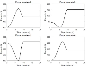
quintic polynomial has been used to generate the desired values of x, y, z and γ in order to guarantee a smooth trajectory. The time to reach the final point from the initial start point was set at 10 seconds. The performance of the controller after reaching the final point is also analysed to verify if it can maintain the position and orientation without any further action. The results obtained are presented below. The cable forces generated to follow the desired trajectory is shown in fig. (3). It is seen that the values of the forces are positive and within the limits defined earlier. The values of the position of the moving platform is shown in fig. (4). The variation of orientation is seen in fig. (5). The variation in the values of the 2 parameters which are not controlled by the control law, namely α and β are also shown in fig. (5). It is seen that the values of the orientation angle are also within the limits defined earlier which validates the application of the control law for the CDPR.
Fig. 3: Variation in the cable forces when the end effector moves from (1,1,1) to (2,2,1.5).
Fig. 4: Change in the position of the end effector from (1,1,1) to (2,2,1.5)
Fig. 5: Change in the orientation of the end effector from (1,1,1) to (2,2,1.5)
b) With noise in the measurement of force
A white noise of specified bandwidth was added in the force values calculated to simulate the real-world measurements. A power spectral density of 0.001 was added at a sample time of 0.001 seconds. The simulation was then repeated to verify the effectiveness of the designed control law and the results are presented in the following figures. It is seen from the fig. (6,7,8) that the control law is able to give satisfactory performance in achieving the desired results.
Fig. 6: Variation of the cable forces with noise in the measurement of the forces
Fig. 7: Change in the position of the end effector from (1,1,1) to (2,2,1.5) with noise in the measurement of forces
Fig. 8: Change in the orientation of the end effector from (1,1,1) to (2,2,1.5) with noise in the measurement of forces
6.CONCLUSION
This work demonstrates the implementation of the input-output feedback linearization method to control an underactuated cable-driven parallel robot. It is seen from the results that the control law works satisfactorily and can be implemented for the control of the CDPR. However, there is scope to further improve this work by analysing the zero dynamics of the CDPR. Analysing the behaviour of the control law at points closer to the singularity region, tracking of different trajectories by varying outputs individually and analysing the robustness of the control law will be done in the further works. Validation of the control law on the prototype will help us in verifying the law and thus will help in the improvement of the control.
ACKNOWLEDGEMENT
This research is part of the Robotix Academy funded by INTERREG V-A Grand Region program.
REFERENCES
Abbasnejad, G., Carricato, M., (2015). Direct Geometrico-static Problem of Underconstrained Cable-Driven Parallel Robots With n Cables. IEEE Transactions on
Robotics, 31(2), pp. 468–478.
Albus, J., Bostelman, R., Dagalakis, N., (1993). The NIST robocrane. Journal of Robotic Systems 10(5), pp. 709–724.
Alp, A.B., Agrawal, S.K., (2002). Cable suspended robots: Feedback controllers with positive inputs, In:
American Control Conference, 2002. Proceedings of the 2002. IEEE, pp. 815–820.
Diao, X., Ma, O., (2009). Vibration analysis of cable-driven parallel manipulators. Multibody System Dynamics, 21(4), pp. 347–360.
Gosselin, C., (2014). Cable-driven parallel mechanisms: state of the art and perspectives. Mechanical Engineering
Reviews, 1(1), pp. DSM0004-DSM0004.
Gosselin, C., Ren, P., Foucault, S., (2012). Dynamic trajectory planning of a two-DOF cable-suspended parallel robot, In: Robotics and Automation (ICRA), 2012
IEEE International Conference On. IEEE, pp. 1476–
1481.
Higuchi, T., (1988). Application of multi-dimensional wire crane in construction, In: Proc. 5th Int. Symp. on
Robotics in Construction, (Vol. 661).
Hwang, S.W., Bak, J.-H., Yoon, J., Park, J.H., Park, J.-O., (2016). Trajectory generation to suppress oscillations in under-constrained cable-driven parallel robots.
Journal of Mechanical Science and Technology,
30(12), pp. 5689–5697.
Isidori, A., (2013). Nonlinear control systems, Third edition, Communications and control engineering. Springer, London.
Kim, W.H., (1991). Feedback Linearization of Nonlinear Systems: Robustness and Adaptive Control.
Kumar, A.A., Antoine, J.-F., Zattarin, P., Abba, G., (2019). Workspace Analysis of a 4 Cable-Driven Spatial Parallel Robot, In: Arakelian, V., Wenger, P. (Eds.),
ROMANSY 22 – Robot Design, Dynamics and Control. Springer International Publishing, Cham,
pp. 204–212.
Landsberger, S.E., (1985). A new design for parallel link manipulators, In: Proc. of the IEEE International
Conference on Systems. pp. 812–814.
Maier, T., Woernle, C., (1999). Flatness-based control of
underconstrained cable suspension manipulators.
Merlet, J., Daney, D., (2010). A portable, modular parallel wire crane for rescue operations, In: Robotics and
Automation (ICRA), 2010 IEEE International Conference On. IEEE, pp. 2834–2839.
Ming, A., (1994). Study on Multiple Degree-of-Freedom Positioning Mechanism Using Wires (Part I)-Concept, Design and Control. International Journal
of the Japan Society for Precision Engineering,
28(2), pp. 131–138.
Oh, S.-R., Agrawal, S.K., (2006). Generation of feasible set points and control of a cable robot. IEEE
Transactions on Robotics. 22(3), pp. 551–558.
Park, J., Kwon, O., Park, J.H., (2013). Anti-sway trajectory generation of incompletely restrained wire-suspended system. Journal of Mechanical Science
and Technology, 27(10), pp. 3171–3176.
Verhoeven, R., (2004). Analysis of the workspace of
tendon-based Stewart platforms. (Doctoral dissertation,
Universität Duisburg-Essen, Fakultät für Ingenieurwissenschaften, Maschinenbau und Verfahrenstechnik)
Zi, B., Duan, B.Y., Du, J.L., Bao, H., (2008). Dynamic modeling and active control of a cable-suspended parallel robot. Mechatronics, 18(1), pp. 1–12.