HAL Id: hal-00329281
https://hal.archives-ouvertes.fr/hal-00329281
Submitted on 1 Jan 2003
HAL is a multi-disciplinary open access
archive for the deposit and dissemination of
sci-entific research documents, whether they are
pub-lished or not. The documents may come from
teaching and research institutions in France or
abroad, or from public or private research centers.
L’archive ouverte pluridisciplinaire HAL, est
destinée au dépôt et à la diffusion de documents
scientifiques de niveau recherche, publiés ou non,
émanant des établissements d’enseignement et de
recherche français ou étrangers, des laboratoires
publics ou privés.
observations of the ionospheric response to flux transfer
events observed by the Cluster spacecraft at the
high-latitude magnetopause
J. A. Wild, S. E. Milan, S. W. H. Cowley, M. W. Dunlop, C. J. Owen, J. M.
Bosqued, M. G. G. T. Taylor, J. A. Davies, M. Lester, N. Sato, et al.
To cite this version:
J. A. Wild, S. E. Milan, S. W. H. Cowley, M. W. Dunlop, C. J. Owen, et al.. Coordinated
interhemi-spheric SuperDARN radar observations of the ionointerhemi-spheric response to flux transfer events observed
by the Cluster spacecraft at the high-latitude magnetopause. Annales Geophysicae, European
Geo-sciences Union, 2003, 21 (8), pp.1807-1826. �hal-00329281�
Annales
Geophysicae
Coordinated interhemispheric SuperDARN radar observations of
the ionospheric response to flux transfer events observed by the
Cluster spacecraft at the high-latitude magnetopause
J. A. Wild1, S. E. Milan1, S. W. H. Cowley1, M. W. Dunlop2,†, C. J. Owen3, J. M. Bosqued4, M. G. G. T. Taylor3,*, J. A. Davies1, M. Lester1, N. Sato5, A. S. Yukimatu5, A. N. Fazakerley3, A. Balogh2, and H. R`eme4,†
1Department of Physics & Astronomy, University of Leicester, Leicester LE1 7RH, UK 2Blackett Laboratory, Imperial College, London SW7 2BZ, UK
3Mullard Space Science Laboratory, University College London, Holmbury St. Mary, Dorking, Surrey RH5 6NT, UK 4CESR, BP 4346, 31028 Toulouse 4, France
5National Institute of Polar Research, Tokyo 173-8515, Japan
*now at: Los Alamos National Laboratory, Los Alamos, NM 87545, USA
†now at: Rutherford Appleton Laboratory, Chilton, Didcot, Oxfordshire, OX11 0QX, UK
Received: 28 October 2002 – Revised: 10 March 2003 – Accepted: 25 March 2003
Abstract. At 10:00 UT on 14 February 2001, the
quar-tet of ESA Cluster spacecraft were approaching the North-ern Hemisphere high-latitude magnetopause in the post-noon sector on an outbound trajectory. At this time, the interplan-etary magnetic field incident upon the dayside magnetopause was oriented southward and duskward (BZnegative, BY
pos-itive), having turned from a northward orientation just over 1 hour earlier. As they neared the magnetopause the mag-netic field, electron, and ion sensors on board the Cluster spacecraft observed characteristic field and particle signa-tures of magnetospheric flux transfer events (FTEs). Follow-ing the traversal of a boundary layer and the magnetopause, the spacecraft went on to observe further signatures of FTEs in the magnetosheath. During this interval of ongoing pulsed reconnection at the high-latitude post-noon magnetopause, the footprints of the Cluster spacecraft were located in the fields-of-view of the SuperDARN Finland and Syowa East radars located in the Northern and Southern Hemispheres, re-spectively. This study extends upon the initial survey of Wild et al. (2001) by comparing for the first time in situ magnetic field and plasma signatures of FTEs (here observed by the Cluster 1 spacecraft) with the simultaneous flow modulations in the conjugate ionospheres in the two hemispheres. During the period under scrutiny, the flow disturbances in the conju-gate ionospheres are manifest as classic “pulsed ionospheric flows” (PIFs) and “poleward moving radar auroral forms” (PMRAFs). We demonstrate that the ionospheric flows ex-cited in response to FTEs at the magnetopause are not those expected for a spatially limited reconnection region, some-where in the vicinity of the Cluster 1 spacecraft. By examin-ing the large- and small-scale flows in the high-latitude iono-sphere, and the inter-hemispheric correspondence exhibited during this interval, we conclude that the reconnection pro-cesses that result in the generation of PIFs/PMRAFs must Correspondence to: J. A. Wild ([email protected])
extend over many (at least 4) hours of magnetic local time on the pre- and post-noon magnetopause.
Key words. Ionosphere (plasma convection) –
Magne-tospheric physics (magnetosphere-ionosphere interactions; magnetospheric configuration and dynamics)
1 Introduction
The exact nature of the coupling mechanism between the so-lar wind and the Earth’s magnetosphere remains one of the key outstanding questions in solar-terrestrial physics. Ob-servations supporting the supposition that reconnection pro-cesses at the high-latitude magnetopause are frequently tran-sient in nature were first presented by Haerendel et al. (1978), exploiting magnetic field measurements from the HEOS-2 spacecraft. Using lower latitude magnetic field observations from the ISEE-1 and 2 spacecraft, Russell and Elphic (1978, 1979) also reported transient signatures of magnetic recon-nection at the magnetopause with time scales of a few min-utes and a recurrence interval of ∼5–10 min, and it was these authors that went on to term these transient signatures “flux transfer events” (FTEs). These transients are usually char-acterised by bipolar signatures in the magnetic field com-ponent normal to the magnetopause (sometimes associated with field tilting effects in the plane of the magnetopause) and a mixed plasma population of both magnetospheric and magnetosheath origin (e.g. Paschmann et al., 1982; Farru-gia et al., 1988). The physical interpretation of FTEs of-fered by Russell and Elphic (1978, 1979) was based upon transient (few minute) and spatially localised (few RE)
vals of magnetic reconnection at the magnetopause, an inter-pretation that was subsequently supported by several studies showing that FTEs were most frequently observed during in-tervals with southward directed fields in the magnetosheath
(e.g. Rijnbeek et al., 1984; Berchem and Russell, 1984; Kawano and Russell, 1997). The size, longevity and evolu-tion of the reconnecevolu-tion site from which FTEs originate has been the subject of much debate; for example, Southwood et al. (1988) and Scholer (1988) postulated that the transient re-connection region extends significantly further over the mag-netopause surface than was originally suggested by Russell and Elphic (1978, 1979) whilst Milan et al. (2000), drawing upon UV auroral imager data and HF radar data, suggested that the reconnection site may at any one time be spatially localised, but that it propagates wave-like over the magne-topause for extended distances and intervals of time (at least
∼10 min).
Clearly, the dayside ionospheric flow response to recon-nection processes at the magnetopause will depend upon the prevailing reconnection geometry at the boundary, and a range of theoretical descriptions have been proposed to describe the expected flow signatures that would result from patchy, extended, or wave-like reconnection sites (e.g. Southwood, 1985, 1987; Cowley, 1986; McHenry and Clauer, 1987; Lockwood et al., 1990; Wei and Lee, 1990; Cowley et al., 1991; Cowley and Lockwood, 1992; Milan et al., 2000). Motivated by the potential to exploit iono-spheric observations in order to diagnose reconnection pro-cesses at the magnetopause, a great deal of effort has been made to observe the signatures of FTEs in the high-latitude ionosphere. Among the first ground-based measurements to be interpreted as potential flux transfer events were those of van Eyken et al. (1984), who reported a brief northward excursion in a westward flow region observed by the EIS-CAT UHF incoherent scatter radar. Subsequently, Lock-wood et al. (1989, 1993) associated ionospheric flow en-hancements observed by the EISCAT system with dayside auroral transients that related to FTEs observed at the magne-topause. In recent years high frequency (HF) coherent radars have provided a wealth of observations that have been as-sociated with flux transfer events. HF radars often observe high velocity antisunward transient flow in the cusp iono-sphere and it was these signatures that were interpreted as the response to transient magnetopause reconnection by Pin-nock et al. (1993, 1995) and Rodger and PinPin-nock (1997). Subsequently, quasi-periodic sequences of such events, of-ten termed “pulsed ionospheric flows” (PIFs), have been re-ported and examined both individually (Provan et al., 1998) and statistically (Provan and Yeoman, 1999). These are often also seen as poleward-moving regions of enhanced backscat-ter power, the radar counbackscat-terpart of “poleward-moving auroral forms” (PMAFs), widely accepted to be the auroral signa-ture of FTEs (e.g. Sandholt et al., 1990; Thorolfsson et al., 2000). In the text below we will refer to these radar PMAFs as “poleward-moving radar auroral forms” or PMRAFs. As noted by Wild et al. (2001), care should be taken in the use of “PIF” and “PMRAF” nomenclature, which are often er-roneously used interchangeably. It is not always possible to say whether isolated PMRAFs are associated with a PIF or not, as no measurements of the ionospheric flow preceding or following the PMRAF are made (as no backscatter is
ob-served). The lack of backscatter before or after the PMRAF does not necessarily indicate that a change in convection flow has occurred, only that no targets were present from which the radar could scatter. However, the almost continuous ob-servations of the polar ionosphere provided by HF coherent radars have enabled the spatial extent of these events, their flow orientation, MLT occurrence, dependence on IMF ori-entation, and repetition frequencies to be extensively exam-ined (Provan et al., 1998, 1999; Provan and Yeoman, 1999; Milan et al., 1999, 2000; McWilliams et al., 2000).
Employing ionospheric flow observations from the EIS-CAT radar system and magnetic field measurements from the ISEE-1 and -2 spacecraft, Elphic et al. (1990) presented the first simultaneous observations of an FTE at the mag-netopause and the flow response in the near-conjugate iono-sphere. More recently, Neudegg et al. (1999) presented the first coordinated space- and ground-based study of FTEs to exploit measurements from a HF coherent radar system. Dur-ing the case study presented, a southward turnDur-ing of the IMF resulted in the observation of a clear magnetospheric FTE in the magnetometer data of the Equator-S spacecraft, lo-cated in the vicinity of the low-latitude morning-sector mag-netopause. The timing of the observed FTEs closely matched the onset of transient poleward-propagating flow features in the SuperDARN Hankasalmi (CUTLASS) radar. It is worth noting that since this study employed data acquired using a non-standard radar mode, the ionospheric flow data pre-sented was of exceptionally high quality with better than usual spatial and temporal resolution. This allowed the au-thors to accurately deduce the resulting ionospheric convec-tion, which proved to be consistent with previous HF radar results based solely upon ground-based data. Neudegg et al. (2001) went on to show that the high-latitude convec-tion response to the reconnecconvec-tion process associated with this magnetopause FTE excited strong UV aurora equatorward of the footprint of the newly-reconnected field lines. By carry-ing out a statistical survey of FTEs observed in the vicinity of the magnetopause by the Equator-S spacecraft, Neudegg et al. (2000) found a strong association with the characteristic pulsed antisunward flows observed in the HF radar data at the conjugate ionospheric footprint of the spacecraft. They went on to suggest that for FTEs with a repetition rate of greater than ∼5 min, a clear one-to-one correlation often existed be-tween magnetopause and ionospheric events. For faster rep-etition rates, the ionospheric response began to resemble that expected from a continuous flow excitation. The overall flow patterns observed in association with the FTEs were in broad agreement with those predicted theoretically, but showed a wide variety of responses on an event-to-event basis.
Combining, for the first time, magnetic field observations from the ESA Cluster mission and ground-based coherent-and incoherent-scatter radar measurements of the iono-spheric flow in the region of the dayside cusp, Wild et al. (2001) presented simultaneous observations of FTEs at the high-latitude magnetopause and pulsed radar signatures in the conjugate Northern Hemisphere ionosphere. More specifically, transient bipolar signatures in the magnetic field
component normal to the magnetopause, characteristic of FTEs at the high-latitude magnetopause, were observed to coincide with pulsations in the ionospheric flow at the lat-itude of the Cluster footprint measured by the Hankasalmi SuperDARN (CUTLASS) HF radar. The radar features pul-sated in both velocity and backscatter power and were ob-served propagating poleward, forming classic “pulsed iono-spheric flow” (PIFs) and “poleward-moving radar auroral forms” (PMRAFs) at higher latitudes. Furthermore, Wild et al. (2001) demonstrated an excellent correspondence be-tween the FTEs observed at the magnetopause and the pul-sations in the dawnward component of the ionospheric flow despite the radar measurements being displaced by some 2 h of MLT to the west of the estimated location of the Clus-ter footprint. Considering the expected dawnward and pole-ward motion of reconnected flux tubes in the Northern Hemi-sphere post-noon magnetoHemi-sphere due to the duskward and southward directed IMF during the interval presented, it was suggested by Wild et al. (2001) that the lower latitude west-ward flow region corresponded to newly-opened flux tubes in which the first influences of each burst of reconnection were felt. In addition, an apparent relationship between the zonal ionospheric flow modulation and PIF/PMRAF signatures at higher latitudes was reported. More specifically, enhance-ments in backscattered power observed in the lower-latitude westward flow region generally preceded PIF or PMRAF sig-natures at higher latitudes, implying that the PIF/PMRAF events originated near a latitude of 74◦–75◦(close to the lat-itude of the Cluster footprint) and propagated poleward to
∼80◦ where they resembled the more classic PIF/PMRAF signatures. An association between flow changes at lower latitudes and PMRAF features at higher latitudes had pre-viously been reported in studies by Milan et al. (2000) and Davies et al. (2002). Consequently, Wild et al. (2001) went on to concluded that PMRAFs are “fossils” of the iono-spheric structuring that takes place at the ionoiono-spheric foot-print of the dayside merging gap and as such are useful trac-ers of the convection flow on newly-reconnected field lines. The occurrence of these fossils in relation to PIFs may yield information regarding the level of inductive smoothing of the flow being excited by the reconnection process. Signif-icantly, it was suggested that the observation of a PMRAF might be delayed from its associated burst of reconnection by up to several minutes.
The data presented in Wild et al. (2001) (hereafter re-ferred to as Paper 1), were drawn from the first two weeks of Cluster science operations and constituted a “first results” overview of the interval 09:15–11:15 UT on 14 February 2001. Since the preparation of Paper 1 a substantially ex-tended dataset, from both space- and ground-based instru-ments, has become available and has allowed for a more comprehensive investigation of the interval to be undertaken. This paper will present hitherto unique simultaneous inter-hemispheric ground-based observations of the response to FTEs observed at the magnetopause by Cluster; a compre-hensive multi-spacecraft, multi-instrument in situ study of the FTEs observed at the high-latitude magnetopause during
this interval will be presented in a future companion paper.
2 Instrumentation
2.1 SuperDARN radar data
The Super Dual Auroral Radar Network (SuperDARN) (Greenwald et al., 1995) comprises 15 HF coherent-scatter radars covering a large fraction of the auroral zone and polar cap in each hemisphere (nine in the Northern Hemisphere and six in the Southern Hemisphere). Each radar is fre-quency agile in the range 8–20 MHz, although they most commonly operate at frequencies in the 10–14 MHz range, scattering multi-pulse sequences of HF radio waves from de-cametre scale electron density irregularities in the E- and F-region ionosphere. By employing phased arrays of anten-nas, the radars are able to electronically steer the transmit-ted pulse sequence, sounding 16 beams (each separatransmit-ted by 3.24◦in azimuth) with each beam subdivided into 75 range gates. During the interval of interest, all 15 SuperDARN radars were operating in a common mode in which each beam was sounded for 3 s, thus completing a full scan of all 16 beams (some 52◦ in aziumth) every 1 min, the shortfall being used for the processing and recording of data and to en-able all fifteen radars to “synchronize” and begin successive scans at predetermined times (such as minute boundaries). The length of each of the 75 gates was set to 45 km with a range to the first gate of 180 km. In addition to measuring the backscattered power received at the radar, Doppler spec-tra are obtained by analysing the autocorrelation function of the returned signals, from which the mean Doppler velocity, an estimate of the line-of-sight (l-o-s) plasma velocity, and Doppler spectral width are derived.
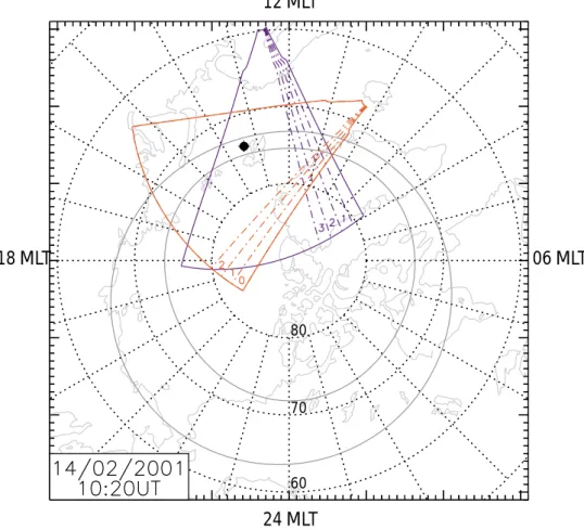
This study presents l-o-s backscattered power and Doppler velocity observations from two SuperDARN radars, namely the Finland and Syowa East radars. The Finland radar is located at Hankasalmi (62.3◦N, 26.6◦E) and forms part of the Co-operative UK Twin Located Auroral Sounding Sys-tem (CUTLASS); the Syowa East radar is sited close to the Syowa station (69.0◦S, 39.6◦E) in Antarctica. Figure 1 presents the fields-of-view (f-o-v) of these radars in an MLT-magnetic latitude coordinate system. The north MLT-magnetic pole lies at the centre of the figure with lines of constant magnetic latitude at 10◦increments indicated by concentric dotted circles. The dotted radial lines represent meridians of magnetic local time at one hour increments, with mag-netic midnight (noon) being located at the bottom (top) of the figure and dawn (dusk) located on the right-(left-) hand side. For reference, the statistical location of the auroral oval (Feldstein and Starkov, 1967) for the appropriate level of ge-omagnetic activity (Kp =4) and the coastlines of the
North-ern Hemisphere land masses at 10:20 UT on 14 February 2001 have been overlaid. The overall f-o-v of the Finland radar at this time is represented by the solid blue lines with the locations of three individual beams discussed in detail be-low indicated by dot-dashed blue lines and numbered
accord-Figure 1
24 MLT
18 MLT 06 MLT
12 MLT
80° 70° 60°Fig. 1. A magnetic latitude-magnetic local time projection of the Northern Hemisphere at 10:20 UT on 14 February 2001. Lines of constant
geomagnetic latitude, starting at 80◦N and then at 10◦intervals, are indicated by dotted concentric circles. Magnetic local time meridians at 1 h intervals are also indicated by dotted lines with magnetic noon (midnight) located at the top (bottom) of the figure and dawn (dusk) located on the right- (left-) hand side. The Northern Hemisphere coastlines at this time are indicated in light grey and the statistical location of the auroral oval (Kp=4) by solid dark grey lines. The overall field-of-view of the SuperDARN Finland radar is shown by the solid indigo lines.
The individual beams within the field-of-view referred to in the text are bounded by dot-dashed lines and numbered appropriately. Similarly, the field-of-view and specific beams of the Southern Hemisphere SuperDARN Syowa East radar, mapped into the Northern Hemisphere, are also indicated by red solid and dot-dashed lines, respectively. The Northern Hemisphere ionospheric footprint of the Cluster 1 spacecraft at this time is indicated by the crossed circle.
ingly. Similarly, the overall f-o-v and three individual beams of the Southern Hemisphere Syowa East radar, mapped into the Northern Hemisphere, are indicated by red solid and dot-dashed lines respectively. Finally, the magnetic footprint of the Cluster 1 spacecraft at 10:20 UT on 14 February 2001 is shown in Fig. 1 by the black crossed circle. This footprint was mapped from the location of the Cluster 1 spacecraft us-ing the Tsyganenko-96 magnetic field model (Tsyganenko 1995, 1996) and parameterised as discussed below.
In addition to the measurements of l-o-s Doppler veloc-ity from the Finland and Syowa East radars, observations of ionospheric flow from all the available SuperDARN radars (in both hemispheres) are employed to estimate the large-scale ionospheric convection pattern using the “map poten-tial” technique of Ruohoneimi et al. (1996, 1998). This tech-nique is discussed more fully below.
2.2 ACE interplanetary data
The IMF and solar wind parameters required for this study were measured by the MAG and SWEPAM instruments re-spectively, on board the Advanced Composition Explorer (ACE) spacecraft (McComas et al., 1998; Smith et al., 1998; Stone et al., 1998), located some 237 RE upstream from the
Earth during the interval of interest. The propagation de-lay between field signatures appearing at the ACE spacecraft and their arrival at the subsolar magnetopause has been es-timated using the technique of Khan and Cowley (1999). In summary, this method takes into account the propaga-tion of IMF features with the solar wind to the bow shock and then across the magnetosheath to the magnetopause, us-ing empirical model values of the location of these bound-aries controlled by the observed solar wind parameters. For conditions during the period of interest (nSW∼1–3 cm−3,
∼55 min. For example, the IMF and solar wind parameters input to the magnetic field and boundary models presented in Fig. 2 and corresponding to 10:20 UT on 14 February 2001 are those measured at the ACE spacecraft at 09:25 UT on the same date, these being Pdyn = 1.5 nPa, IMF BY =2.8 nT,
and IMF BZ = −2.5 nT. Similarly, the ACE data presented
below have been lagged by 55 min so that they may be com-pared with Cluster observations near the magnetopause. The appropriate values of the Dst and Kpindices at the time were
37 nT and 4, respectively, indicating moderate levels of geo-magnetic activity.
2.3 Cluster data
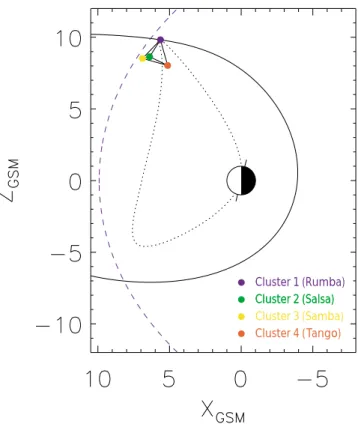
Figure 2 presents the motion of the Cluster 1 (Rumba) space-craft in the GSM X − Z plane during the interval from 14:00 UT on 13 February 2001 to 18:00 UT on 14 Febru-ary 2001. At this time, the apogee of the Cluster orbit was located at around 13:00 MLT, with the spacecraft passing through slightly earlier local times during their inbound mo-tion in the Southern Hemisphere and slightly later local times in the Northern Hemisphere moving outbound from perigee. The locations of the Cluster 1, 2, 3, and 4 spacecraft relative to the Cluster 1 orbital path at 10:20 UT on 14 February 2001 are indicated by indigo, green, yellow and red filled circles, respectively. The inter-spacecraft separation has been exag-gerated by a factor of 20, in order to emphasise the tetra-hedral configuration of the quartet during this interval. A cut though a Shue et al. (1997) model magnetopause at the approximate location of the Cluster 1 spacecraft out of the GSM X − Z plane (YGSM≈3.9 RE) at 10:20 UT is indicated
by the dashed indigo line. The magnetospheric field passing through the Cluster 1 spacecraft at this time inferred from the Tsyganenko-96 field model (Tsyganenko 1995, 1996) is also included, represented by the dotted black line. Both the model magnetopause location and magnetospheric field line model are parameterised by solar wind and IMF conditions. The Shue et al. (1997) magnetopause location and shape is controlled by the solar wind dynamic pressure Pdyn, and the
BZ component of the IMF whilst the Tsyganenko-96 field
model utilises these and a further two parameters, namely the
BY component of the IMF and the Dst index. Consequently,
the solar wind and IMF parameters employed to generate this figure are those quoted above.
The Cluster fluxgate magnetometer (FGM) experiment (Balogh et al., 1997, 2001) comprises two triaxial fluxgate magnetic field sensors on each of the four spacecraft (eight in total). In normal operation the outboard sensor, located at the end of a 5 m boom, is used as the primary source of data. The FGM sensors are calibrated such that the local magnetic field vector can be measured with an accuracy approaching 0.1 nT at high sample rates (up to 67 vectors s−1). The FGM magnetic field data presented in this study were recorded by spacecraft 1 (Rumba) and have been analysed at a temporal resolution equal to the spin period of the spacecraft (∼4 s).
Observations of the ion populations encountered by the Cluster spacecraft are provided by the Cluster Ion
Spectrom-Cluster 1 (Rumba) Cluster 2 (Salsa) Cluster 2 (Salsa) Cluster 3 (Samba) Cluster 4 (Tango) Figure 2
Fig. 2. Plot showing the projection of the orbit of the Cluster 1
(Rumba) spacecraft on to the GSM X − Z plane during the inter-val 14:00 UT on 13 February 2001 to 18:00 UT on 14 February 2001. The relative locations of the four spacecraft at 10:20 UT on 14 February are indicated by coloured circles, as described by the key, where the separation from Cluster 1 has been magnified by a factor of 20, in order to more clearly demonstrate the tetrahedral formation. This time also corresponds the Northern Hemisphere map presented in Fig. 1. A Tsyganenko-96 model field line, as de-scribed in the text, has been drawn from the location of the Clus-ter 1 spacecraft (black dotted line). In addition, a cut through the model magnetopause at YGSM ≈ 3.9 RE (the approximate
loca-tion of Cluster 1 at 10:20 UT) is indicated by the dashed blue line, whilst the orientation of the Earth’s magnetic dipole is indicated by the short black lines.
etry (CIS) experiment (R`eme et al., 1997, 2001). This instru-ment is able to measure the full three-dimensional ion distri-bution of the major magnetospheric ions, namely H+, He+, He++, and O+, from thermal energies to about 40 keV/e. The CIS experiment on board each of the Cluster space-craft comprises two separate instruments: a COmposition and DIstribution Functions analyser (known as CODIF or CIS1) and a Hot Ion Analyser (HIA/CIS2). The CODIF in-strument is capable of measuring the mass per charge com-position of the ion population with medium (22.5◦) angular resolution, whereas the HIA instrument offers no mass res-olution but has superior angular resres-olution (5.6◦). The CIS data presented below were recorded by the HIA instrument on board the Cluster 1 spacecraft and are presented at two different temporal resolutions. First, moments of the three-dimensional distribution yielding the total ion number
den-sity (assuming that all measured ions are H+) are calculated
on board the spacecraft at spin (∼4 s) resolution; secondly, energy-time ion spectrograms are retrospectively generated from the three-dimensional distributions acquired over three spins of the spacecraft (12 s).
The electron observations in the vicinity of the high-latitude magnetopause included in this study were made by the Cluster Plasma Electron And Current Experiment (PEACE) (Johnstone et al., 1997; Owen et al., 2001). Each PEACE instrument (one per spacecraft) is equipped with two sensor heads, a Low- and a High-Energy Electron Analyser (LEEA and HEEA, respectively), which are mounted on op-posite sides of the spacecraft, each of which is capable of measuring electrons in the energy range 0.7 eV to ∼30 keV, arriving from all directions during a spacecraft spin. During the interval presented, the PEACE instrument was configured such that each sensor measured a subset of the maximum possible energy range with HEEA covering the upper part of the energy range. Accordingly, the PEACE data included be-low shows electron fluxes averaged over all look-directions of the HEEA sensor on board the Cluster 1 spacecraft and has a temporal resolution equal to the spacecraft spin period (∼4 s).
3 Observations
This paper focuses on ground-based radar observations of the ionosphere, in both hemispheres, during a period when mag-netic reconnection was occurring at the high-latitude dayside magnetopause, characterised by the observation of a series of FTEs by the Cluster spacecraft. In order to examine the ionospheric response to the inferred magnetospheric dynam-ics, it is first necessary to present the in situ observations of FTEs in the vicinity of the magnetopause, and then show the ground-based observations of the ionospheric flows that sub-sequently arose. However, as the in situ field and plasma observations introduced in this section will be the subject of a rigorous, multi-spacecraft, multi-instrument investigation to be published in a future companion study, this paper will present an overview of the in situ data drawn from one Clus-ter spacecraft only (ClusClus-ter 1).
3.1 Cluster observations
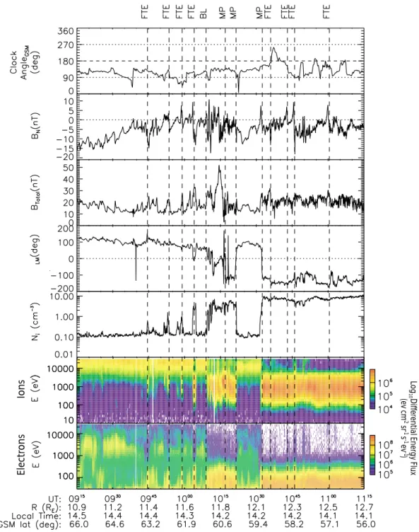
Figure 3 presents observations of the local magnetic field and particle environment at the Cluster 1 spacecraft during the in-terval 09:15–11:15 UT on 14 February 2001, which includes the outbound passage from the magnetosphere to the mag-netosheath. Also displayed (upper panel) is the clock angle of the IMF measured upstream of the Earth and lagged by 55 min, as discussed above. Since the upstream IMF con-ditions and the magnetic field measured by the four Cluster spacecraft during this passage were discussed in detail in Pa-per 1, only a short review is presented here, in order to place the newly available plasma observations in the context of the
magnetic field and ground-based signatures of FTEs reported by Wild et al. (2001).
Immediately prior to the interval discussed here, the IMF was oriented northward with a significant dawnward com-ponent (BY negative, BZ positive). Following a
reorien-tation at around 08:53 UT (lagged time) the IMF was di-rected predominantly southward (BZ∼−3 nT) and duskward
(BY∼5 nT) during the interval presented, with corresponding
IMF clock angles in the range 90–180◦, with the exception of a few brief excursions into northward or dawnward orienta-tions. The magnitude of the IMF remained generally steady throughout, varying slightly between 6 nT at the beginning of the interval and 5 nT toward the end.
The three panels beneath the ACE IMF data present ob-servations from the FGM instrument on board the Cluster 1 spacecraft. As is usual when presenting magnetic field ob-servations from the region adjacent to the magnetopause, the data are presented in a boundary-normal coordinate system (Russell and Elphic, 1978), where N is the estimated out-ward normal to the magnetopause, L lies in the boundary and points north (such that the L − N plane contains the GSM Z axis), and M also lies in the boundary and points west, orthogonal to L and N (such that (L, M, N ) forms a right-handed coordinate system). The first of these panels presents the BNcomponent of the observed field, the second
panel presents the total field magnitude, whilst the third panel shows the angle of the field in the plane of the magnetopause,
αLM, defined as αLM =tan−1(BM/BL). In order to present
magnetic field data in this coordinate system, it is, of course, first necessary to estimate the outward magnetopause normal direction. In order to obtain a representative outward normal direction for the magnetopause encountered during the cen-tral portion of the interval presented in Fig. 3, the minimum variance analysis technique (Sonnerup and Cahill, 1967) was applied to the interval 10:00–10:40 UT, yielding an outward unit normal given by GSM components (+0.669, −0.262,
+0.696). For a more detailed discussion regarding the de-termination of this normal direction, the reader is directed to Paper 1.
The fifth and sixth panels of Fig. 3 present the total ion concentration and energy-time spectrogram measured by the CIS HIA instrument on Cluster 1, respectively. Finally, the lower panel presents an energy-time spectrogram of electrons observed by the HEEA sensor of the PEACE instrument, also on board the Cluster 1 spacecraft.
At 09:15 UT on 14 February 2001 (the beginning of the interval shown in Fig. 3) the Cluster 1 spacecraft was lo-cated within the magnetosphere at a radial distance of ap-proximately 10.9 RE from the Earth and moving on an
out-bound trajectory toward the high-latitude post-noon mag-netopause. The observed magnetospheric field strength at this time was ∼20 nT and directed mainly southward and westward (BL negative, BM positive), as expected in the
vicinity of the post-noon cusp. By 11:15 UT, the Cluster 1 spacecraft had passed into the magnetosheath, the field be-ing oriented southward and eastward (BLand BM negative)
Ions Elec tr ons α Figure 3 -2 -1 -1 -1 10 L o g Diff er ential Ener gy F lux (ev cm sr s ev )
Fig. 3. Plot of ACE and Cluster data for the interval 09:15–11:15 UT on 14 February 2001. The top panel shows the clock angle of
the interplanetary magnetic field measured at the ACE spacecraft and lagged by 55 min such that comparisons can be made with the Cluster observation at the front of the magnetosphere. The next three panels present the component of the magnetic field normal to the magnetopause, the total magnetic field strength, and the angle of the magnetic field in the plane of the magnetopause (the αLM parameter) measured by the
FGM instrument on board the Cluster 1 (Rumba) spacecraft. The fifth and sixth panels present the total ion density profile and ion energy-time spectrogram (all pitch angles) observed by the CIS2 (HIA) instrument on Cluster 1. Finally, the lower panel presents the electron energy distribution measured in the field-parallel direction by the PEACE HEEA sensor, also on Cluster 1. Overlaid on this figure (dashed lines) are the times of events originally identified by Wild et al. (2001) and discussed in the text. Specifically, the centre times of four magnetospheric FTEs, the entry into the boundary layer (BL), three crossings of the magnetopause (MP), and four magnetosheath FTEs are indicated.
the expected orientation of the field in the magnetosheath based upon upstream IMF conditions. Plasma observations from the CIS and PEACE instruments also clearly indicate
the transition from magnetosphere- to magnetosheath-like plasma over the interval presented. The magnetospheric ion concentration measured by CIS at the beginning of the
interval was ∼ 0.1 cm−3, with the energy at the peak ion flux greater than ∼10 keV. This is compared to the observed ion concentration of ∼10 cm−3in the magnetosheath, where the peak of ion energy distribution is significantly lower (∼1 keV). This transition from a hot, tenuous plasma to a cooler, denser plasma was reflected in measurements of the electron population made by PEACE, which recorded a shift in the energy of the peak flux of the electron distribution from a few keV in the magnetosphere to several tens of eV in the magnetosheath.
The timings of several key features identified in Paper 1 are indicated by dashed lines in the central portion of the interval displayed in Fig. 3. At 10:09 UT, some 8 min prior to the first magnetopause encounter, the spacecraft encountered a boundary layer (marked “BL”) in which the magnetic field became increasingly variable, but generally veered toward the direction of the field in the magnetosheath. Three clear magnetopause crossings followed (labelled “MP”) occurring at ∼10:17 UT (magnetosphere-magnetosheath), ∼10:22 UT (magnetosheath-magnetosphere), and ∼10:33 UT (magneto-sphere-magnetosheath).
Plasma observations, unavailable to us during the prepa-ration of Paper 1, support our interpretation of three mag-netopause transitions, the first of which was preceded by observations of a boundary layer lasting several minutes. At ∼10:09 UT CIS recorded an approximate factor of 20 increase in the ion concentration at the Cluster 1 space-craft. Although variable over the next few minutes, this en-hanced ion concentration peaked at ∼7 cm−3before settling at slightly lower values until just prior to the first magne-topause crossing at ∼10:17 UT. This increase in concentra-tion was accompanied by a marked change in the ion popula-tion energy distribupopula-tion from magnetosphere-like (∼10 keV) to more magnetosheath-like energies (several hundred eV to a few keV). Significant structure, some of which appears to be energy dispersed, is also apparent within the bound-ary layer. Following the first penetration of the magne-topause at ∼10:17 UT, the observed plasma population was magnetosheath-like in terms of ion concentration, ion energy distribution and electron energy distribution. The subsequent magnetopause crossing at ∼10:22 UT returned the spacecraft to a plasma environment that was generally magnetosphere-like in nature until ∼10:33 UT, when the spacecraft again crossed the magnetopause, exiting the magnetosphere for the last time on this pass.
As Cluster 1 approached the magnetopause for the first time, the observed magnetic field became increasingly vari-able in both direction and magnitude. This was particu-larly evident after ∼09:00 UT, when the (lagged) IMF turned southward at the subsolar point. It is, therefore, highly likely that the increased level of variability was directly linked to sustained dynamic processes in the boundary re-gion. The most notable consequences of this are the four clear magnetospheric FTEs marked by the vertical dashed lines, observed at ∼09:45 UT, ∼09:54 UT, ∼09:59 UT, and ∼10:04 UT, prior to the entry into the boundary layer at ∼10:09 UT. These FTEs were characterised by bipolar
positive-to-negative (“normal” polarity) perturbations in the normal component of the magnetic field (BN), and increases
in the overall field strength. In addition, each FTE was accompanied by mixing of the magnetospheric and mag-netosheath plasma populations. The exact nature of this mixing varied between the FTEs, although in general there was an increase in the ion concentration, particularly at magnetosheath-like energies (∼100 eV–5 keV) and, in some cases, a depletion of the more energetic magnetospheric ion population. Similar enhancements of magnetosheath-like plasma were observed in the electron measurements, al-though the depletion of the magnetospheric electron popula-tion was more pronounced than in the case of the ions, pre-sumably reflecting the greater field-aligned mobility of the electrons.
Following the entry of Cluster 1 into the magnetosheath at ∼10:33 UT, further FTEs were observed with those at ∼10:36 UT, ∼10:43 UT, ∼10:46 UT, and ∼11:01 UT (marked by vertical dashed lines), being clear examples of FTE-like bipolar signatures in the magnetic field. These magnetosheath FTEs are also associated with mixing of mag-netosheath and magnetospheric plasma, with the enhance-ment of magnetospheric electrons and ions being particularly prominent during the ∼10:46 UT event.
It is worth noting that analysis of the electron and ion observations now available reveals further evidence of on-going dynamic processes at the high-latitude magnetopause that was not obvious when considering the magnetic field observations alone (as in Paper 1). From the outset of the interval shown in Fig. 3 (almost 1 h prior to the first mag-netopause encounter), there are indications of brief inter-vals of magnetosheath-like ion and electron fluxes and deple-tion of the magnetospheric electron populadeple-tion at Cluster 1. The plasma observations also yield much additional struc-ture associated with the magnetospheric and magnetosheath FTEs. In particular, it is possible to resolve short-lived enhancements in the magnetosheath-like ion and electron fluxes at ∼09:51 UT, ∼09:56 UT, ∼10:02 UT, ∼10:07 UT, and ∼10:27 UT. Once into the magnetosheath proper, addi-tional enhancements in the magnetospheric-like ion and elec-tron populations are apparent at ∼10:50 UT and ∼10:52 UT. Whilst it is not within the scope of this paper to analyse each of these events in detail, it is clear that throughout the inter-val 09:15–11:15 UT on 14 February 2001, magnetic recon-nection was occurring almost continuously at some locations on the dayside magnetopause, which resulted in FTEs being observed at the high-latitude post-noon boundary.
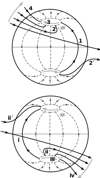
Our interpretation of the field perturbations observed dur-ing these FTE events is shown in Fig. 4a (we shall return to consider Fig. 4b later). This shows a schematic of the day-side magnetopause viewed from the Sun, where the arrowed dashed lines show undisturbed magnetospheric field lines in the magnetopause layer. Magnetic field lines interconnected with the IMF/magnetosheath are indicated by solid arrowed lines. We assume that the field perturbations observed by Cluster were due to bursts of reconnection occurring east-ward and equatoreast-ward of the spacecraft (although, as
dis-cussed below, we do not suggest that reconnection is occur-ring only in this region). In Fig. 4a reconnection is shown occurring at a point somewhere between the equator and the Cluster spacecraft, near the point marked ‘1’ (the exact lo-cation is uncertain). Following reconnection, the combined action of the magnetosheath flow and the magnetic tension of the newly-opened field lines causes them to contract pole-ward and westpole-ward in the Northern Hemisphere, forming a sunward-moving boundary layer at the post-noon sector magnetopause, such as is described, for example, by the sim-ple magnetopause reconnection model of Cowley and Owen (1989). At subsequent times the open field line (shown by the arrowed solid lines) is thus located at positions 2, 3, and 4. It can thus be seen that the effect of the field tension is such as to cause newly-opened flux tubes at the Cluster location (near ‘2’) to rotate towards a poleward and eastward orientation, in both the magnetosphere and magnetosheath. The west-ward and polewest-ward propagation of newly-opened magnetic flux tubes perturb the underlying (closed) magnetospheric flux tubes in the vicinity of Cluster such as to give positive-to-negative bipolar perturbations in the N component in both magnetosphere and magnetosheath (as presented in Fig. 4a of Wild et al., 2001). This scenario is thus qualitatively con-sistent with the sense of the principal FTE field perturbations seen in Fig. 3. The ‘reversed’ and reduced field tilting effects observed in the first three magnetospheric FTEs marked in the figure, compared with the fourth, is taken to be due to the larger distances from the magnetopause in the earlier events, combined with the twisting of the field within the FTE struc-ture, as found in earlier studies of ISEE1/2 data (e.g. Cowley, 1982; Paschmann et al., 1982; Saunders et al., 1984). The FTE structure as a whole is formed from the bundle of open field lines produced by a given propagating burst of recon-nection (Milan et al., 2000; Wild et al., 2001). The twisting is often such that in the outer part of the FTE the field may tilt away from the direction of the field on the other side of the boundary. Such tilts can also be produced in the unrecon-nected field immediately outside the FTE due to the flows induced in the surrounding medium by the passage of the FTE structure (Southwood, 1985; Cowley, 1986).
Whilst this interpretation of an active reconnection region located somewhere in the dusk sector equatorward of the Cluster spacecraft is consistent with the observations, it is not possible to say whether the reconnection X-line lies on the equator or at higher or lower latitudes. Also, the Cluster data yields no information regarding the azimuthal extent of the reconnection region. For example, it is possible that recon-nection is also occurring in the pre-noon sector, as indicated in Fig. 4b. Here, reconnection has been assumed to occur at some general location southward of the equatorial plane re-sulting in a similar evolution of newly-opened field lines to that described in the Northern Hemisphere case presented in Fig. 4a. Obviously, reconnected field lines with footprints in the Northern Hemisphere are dragged tailward (dawnward) by field line tension effects and the motion of the solar wind and consequently away from the Cluster spacecraft.
1
2
3
4
2´
Figure 4i
ii
iii
iv
ii´
a.
b.
Fig. 4. Sketch of the Earth’s dayside magnetopause in a view
look-ing from the Sun, showlook-ing (a) the temporal evolution of an open flux tube (solid lines marked ‘1’–‘4’) following a low-latitude re-connection event in the dusk sector (near ‘1’) and (b) the temporal evolution of an open flux tube (solid lines marked ‘i’–‘iv’) follow-ing a low-latitude reconnection event in the dawn sector (near ‘i’). The grey arrows indicate the direction of open field line motion, in-cluding westward motion in the northern cusp and eastward motion in the southern cusp. The arrowed short-dashed lines indicate mag-netospheric field lines within the magnetopause boundary region. We also indicate the approximate location of the Cluster spacecraft.
3.2 SuperDARN radar observations
Figure 5 presents observations of received backscattered power and l-o-s ionospheric Doppler velocity as functions of magnetic latitude and universal time from selected beams of the Finland (Fig. 5a) and Syowa East (Fig. 5b) SuperDARN radars. These plots indicate backscattered signals that orig-inate from both ionospheric and ground scattering targets, colour coded according to the scales indicated.
Through-Figure 5
Fig. 5. Three pairs of backscatter power and Doppler shift measurements from (a) beams 1, 2, and 3 of the Finland radar and (b) beams 0,
1, and 2 of the Syowa East radar, covering the same time interval as for the Cluster data in Fig. 3. In the Doppler shift panels, velocities are only shown where significant power is observed. Grey backscatter indicates ground backscatter, and negative velocities represent Doppler shifts away from the radar along the line-of-sight. Poleward-moving radar auroral forms (PMRAFs) are indicated by arrows in the upper power panel for each radar; related events are observed in each of the other beams shown. Superimposed on each panel are the times of note identified in the Cluster observations, as in Fig. 3.
out the interval presented, the measured Doppler veloci-ties at both the Finland and Syowa west radars were over-whelmingly negative (flow away from the radars). Conse-quently, the velocity colour scales are such that only negative Doppler shifts are shown; where signals have been identi-fied as groundscatter (by exhibiting low Doppler velocity and narrow Doppler spectral width) the appropriate velocity data are colour-coded grey. Also, attention is drawn to the differ-ences in the colour-scales (both power and velocity) between Figs. 5a and b. This is necessary since the Syowa East radar generally observed stronger returned signals from lower ve-locity (less negative) flows than the Finland radar. For com-parison, the timings of the key FTE and magnetopause en-counters as discussed above and in Paper 1 are overlaid on each panel of Fig. 5.
Beginning with a summary of the Northern Hemisphere observations, first presented in Paper 1, the backscatter in the westernmost portion of the Finland radar f-o-v (i.e. the beams presented) was characterised by a region of groundscatter at magnetic latitudes equatorward of ∼76◦, embedded in which were regions of ionospheric scatter. The l-o-s Doppler ve-locity of this ionospheric scatter of ≤ 300 m s−1away from the radar throughout. After approximately 10:10 UT, a re-gion of ionospheric backscatter developed slightly poleward of this (∼76◦–79◦) in which the l-o-s Doppler velocity was significantly higher (more negative). As discussed in Pa-per 1, inspection of the l-o-s velocity measurements in the region of the estimated footprint of the Cluster spacecraft did not reveal any significant pulsing of the ionospheric flow, probably because the fluctuations did not have a significant component in the l-o-s direction (which was predominantly meridional) of the radar beam. It is the higher-latitude region of backscatter displayed in Fig. 5a that contains the clear-est radar signatures of FTEs, indeed examples of both PM-RAFs and PIFs are apparent during the interval. Two clear examples of PMRAFs (narrow regions of backscatter with negative Doppler velocity propagating ∼2◦poleward over a period of a few minutes) were observed at ∼09:21 UT and 09:41–09:45 UT in beams 1 to 3 of the Finland radar. During the interval 10:10-10:50 UT, several further events were ob-served that could be classified as both PMRAFs and PIFs; the backscatter poleward of ∼76◦latitude during this period was almost continuous but several poleward-moving enhance-ments in the backscattered power associated with elevated l-o-s Doppler velocity were seen. These events are clearest in the backscattered power and Doppler velocity measure-ments from beam 1 and are marked by arrows in the upper panel of Fig. 5a. Finally, two further PMRAFs with similar characteristics to those seen at the beginning of the interval are observed at ∼10:57 UT and ∼11:07 UT, and these are also marked by arrows in Fig. 5a.
Turning now to the newly available measurements from the Syowa East radar (Fig. 5b), it is immediately appar-ent that on this occasion the nature of the backscatter ob-served in the northern and southern conjugate ionospheres were markedly different. The Southern Hemisphere radar observed a region of backscatter in the most poleward
point-ing beams of the f-o-v (beams 0–8) extendpoint-ing from ∼−75◦ to −78◦ magnetic latitude. Unfortunately, this region of
backscatter did not generally include the ionospheric foot-print of the Cluster spacecraft, and the observations pre-sented originate from ∼2◦poleward and ∼1–2 h MLT further west. In comparison to the Northern Hemisphere measure-ments the echoes received at the Syowa East radar were sig-nificantly stronger (higher received signal power), but were associated with generally smaller Doppler shifts. However, as in the Northern Hemisphere, the measured l-o-s Doppler velocities were almost exclusively directed away from the radar (negative Doppler shifts). Of course, it must be re-membered that the pointing direction of the Syowa East radar is quite different from the Finland radar; at ∼75◦ magnetic latitude, the Finland radar beams presented in Fig. 5 (and shown in Fig. 1) point poleward and westward, whereas the Syowa beams (in the opposite hemisphere) point poleward and eastward. Consequently, the negative Doppler shifts ob-served by the Syowa East radar during this interval corre-spond to a poleward and eastward flow component in the Southern Hemisphere (compared to poleward and westward flow component observed by the Finland radar in the North-ern Hemisphere). Also, the presented beams of the Syowa East radar are more azimuthally pointing than those of the Finland radar and are, therefore, more sensitive to the zonal component of the ionospheric flow. In further contrast to the Northern Hemisphere observations, the flow within the backscatter is broadly similar over the latitude range pre-sented (that is to say that the two bands of backscatter ob-served in the Northern Hemisphere, each with substantially different flow characteristics were not matched in the South-ern Hemisphere). Embedded within and extending from the region of Southern Hemisphere backscatter were several ex-amples of PMRAFs/PIFs (indicated by arrows in the power panel for beam 0). Due to the generally lower Doppler ve-locities observed in the Southern Hemisphere (compared to those in the higher latitude band of scatter in the North-ern Hemisphere) the subtle differences between the velocity within the poleward moving structure and the surrounding backscatter are not always obvious, although the PMRAFs are apparent, extending from the poleward edge of the scat-ter at 09:20–09:22 UT, 09:26–09:32 UT, 09:53–09:57 UT, 11:02–11:05 UT, and 11:06–11:10 UT.
In Paper 1, Wild and co-workers demonstrated a pulsing of the flow in the lower latitude band of scatter observed in the Northern Hemisphere. This pulsing was in addition to the PMRAF/PIFS observed at higher latitudes and in the band of scatter that corresponded to the approximate latitude of the Cluster footprint, albeit some 2 h of MLT westward. Fig-ure 6a presents evidence of such pulsing, drawn from beam 3 of the Finland radar (this beam was chosen as it has the longest unbroken series of measurements in the lower lati-tude backscatter region). In order to highlight the l-o-s veloc-ity fluctuations in the lower latitude band of radar backscat-ter, a colour scale with a reduced velocity range compared to that in Fig. 5a has been employed. Using this modi-fied colour scale, the poleward-propagating organisation of
a.
b.
c.
Figure 6
Fig. 6. (a) Velocity data from beam 3 of the Finland radar, in a format similar to that in Fig. 5, but with a revised colour scale which reveals
the pulsing of the line-of-sight flow in the band of lower-latitude scatter. (c) Velocity data from beam 0 of the Syowa East radar, presented in the format of (a), albeit with a different colour scale and a reversed latitude axis. (b) The mean velocity averaged over the latitude range indicated by dashed horizontal lines in (a) and (c) (and given positive values in this case, though in each case the flow is directed away from the radars). The indigo trace corresponds to the Finland average velocities, whilst the red trace corresponds to the Syowa East average velocities. Superimposed on each panel are the times of note identified in the Cluster observations, as in Fig. 3.
the velocity features in the latitude range ∼74.5◦–76.0◦N is clear. In order to further emphasise the velocity pulsations, the average l-o-s Doppler speed between these latitudes (in-dicated by dashed lines) is presented in Fig. 6b. This dis-plays the average flow speed measured in the direction away from the Finland radar (i.e. negative velocities), as indigo circles joined by indigo lines. As reported in Paper 1, the enhancements in the average Doppler velocity measured by
the Finland radar occurred in association with each of the four magnetospheric FTEs, with peak values occurring typi-cally 1-2 min after what had been judged to be the “centre” time of the FTEs inferred from Cluster magnetic field data (indicated by dashed lines in Fig. 6). Of course, depending upon the relative propagation times from the reconnection site over the magnetopause to the spacecraft, along the mag-netic field to the ionosphere, and from then on to the radar
field-of-view, the relative timing of such pulses for individual events will vary slightly. It is expected that these propagation times will typically be ∼1–5 min, therefore, ∼1–2 min dis-placements in either direction are not unexpected, depending upon the various factors influencing the propagation delay in each case. This interpretation is supported by the Cluster plasma observations now available, indeed additional FTE-like events identified from the electron and ion observations discussed above can be related to additional variations in the Finland radar flow observations and may further explain the smaller velocity enhancements between the peaks associated with each of the marked FTEs.
It is worthwhile to compare the average ionospheric flow velocity at the approximate magnetic latitude of the Cluster footprint in the Northern Hemisphere with those at equiva-lent latitudes in the Southern Hemisphere. The red circles and lines in Fig. 6b indicate the corresponding average flow speed measured in the direction away from beam 0 of the Syowa East radar over the latitude range ∼74.5◦–76.0◦ S. These data are drawn from the l-o-s Doppler velocity mea-surements presented in Fig. 6c (and shown in Fig. 5b but with differing velocity and latitude scales). It is immedi-ately apparent that the average flow velocity in the South-ern Hemisphere consists of similar velocity fluctuations to those observed in the Northern Hemisphere (typically
∼200–300 m s−1variations with ∼5–10 min periodicity) but superimposed upon a background flow of ∼300 m s−1. Note also that at the beginning of the interval presented the South-ern Hemisphere radar observed sustained backscatter with flow = 1000 m s−1 directed away from the radar, whilst in the Northern Hemisphere scattering targets were not present. By the end of the interval, the average flow velocity over the
∼74.5◦–76.0◦latitude range in both hemispheres had
con-verged to approximately 400 m s−1(±200 m s−1).
The Northern Hemisphere observations suggest a relation-ship between the FTE signatures observed by Cluster at the high-latitude post-noon magnetopause and enhancements in l-o-s Doppler velocity and power observed in the backscatter echoes. In particular, these enhancements are observed in the lower latitude (∼74.5◦-76.0◦N) westward flow region. As indicated in Fig. 4a, this westward flow is consistent with the expected motion of recently connected magnetic flux tubes as they are dragged dawnward and poleward, first by mag-netic tension effects acting on the kinked field lines, and then by the antisunward motion of the solar wind. It is espe-cially interesting that there is such excellent correspondence between the ground- and space-based observations, despite the measurements of ionospheric flow being made ∼2 h of MLT to the west of the Cluster footprint. It is unfortunate that similar observations could not be made in closer prox-imity to the Cluster footprint. However, as discussed above, the radar look-direction in the ionosphere directly conjugate to the spacecraft was approximately north-south and, there-fore, insensitive to the westward flow variations, and it is expected that the events and associated ground-based signa-tures under study are large in spatial scale. The observation of ionospheric flow modulations some 2 h of MLT westward
of the Cluster footprint in the Northern Hemisphere iono-sphere adds further weight to this supposition. In Paper 1, Wild et al. noted that some ground-based events were ob-served without a clear FTE signature at the Cluster space-craft, such as the Northern Hemisphere PMRAFs observed at ∼09:21 UT and ∼09:41 UT. It was proposed that this was due to the greater displacement of the spacecraft from the magnetopause at the beginning of the interval, with each spacecraft simply too far away from the boundary to ob-served the related FTE signatures. With the benefit of plasma measurements it can be seen that this interpretation (based upon magnetic field measurements alone) is supported by observations of weak enhancements of magnetosheath-like ion and electron fluxes during the period prior to the FTE observed at ∼09:45 UT. Indeed, the ∼09:21 UT PMRAF co-incided with a clear burst of magnetosheath-like ions, a re-gion of elevated magnetosheath-like and depleted magneto-spheric electron fluxes, and bipolar fluctuations in the nor-mal component of the magnetic field. Very brief (∼30 s) bursts of magnetosheath-like electron fluxes were also ob-served around the time of the ∼09:41 UT PMRAF, although it is difficult to resolve distinct enhancements in the ion pop-ulation associated with these features.
The Cluster magnetic field observations and the Northern Hemisphere measurements of ionospheric flow presented in Paper 1 were interpreted as consistent with a propagating burst of low-latitude reconnection that originated near the noon meridian and then propagated to later local times. Once the reconnection patch had propagated sufficiently duskward of the Cluster spacecraft, the dawnward motion of newly-opened flux tubes gave rise to the field-tilting effects apparent in the in situ magnetic field measurements and the propagat-ing transient features in the ground-based measurements of ionospheric flow. Although it was acknowledged that such a propagating burst of reconnection could also propagate to-ward earlier local times, no observations were available to determine whether or not this was actually the case on this occasion.
In order to further elucidate the large-scale ionospheric flow pattern, the perturbations of which have been presented above, we shall employ the “map potential” technique de-veloped by Ruohoniemi and Baker (1998). This technique yields large-scale global convection maps from the l-o-s ve-locity measurements from multiple radars, via mathematical fitting of the data to an expansion of the electrostatic poten-tial in spherical harmonics. First, the l-o-s data are filtered and then mapped onto a polar grid. These “gridded” mea-surements are then used to determine a solution for the elec-trostatic potential distribution that is most consistent with the available measurements. The electric potentials of the solution then represent the plasma streamlines of the mod-elled convection pattern. As backscatter targets (and there-fore l-o-s velocity measurements) are not always available, information from the statistical model of Ruohoniemi and Greenwald (1996), parameterised by IMF conditions, is used to stabilise the solution where no measurements are made. Figure 7 presents the dayside Northern and Southern
Hemi-14 FEBRUARY 2001
09:40:00 - 09:45:00 UT
2000 m/s m/s 0 0 60 65 70 75 80 85 90 A B E F G K T W -33 -21 -21 -9 -9 -9 3 3 15 15 15 09 MLT 15 MLT 00 MLT 12 MLT 06 MLT 18 MLT 03 MLT 21 MLTNORTHERN HEMISPHERE
-60 -65 -70 -75 R -9 3 15 0 -80 -85 -90 H J N -21 -21 -9 -9 -9 -9 3 3 15 15 27 27SOUTHERN HEMISPHERE
09 MLT 15 MLT 12 MLT 06 MLT 18 MLT APL MODEL 4<BT<6 Bz-/By+ +Z +Y (5 nT) (-55 min) Figure 7Fig. 7. Streamlines and vectors of the ionospheric flow derived from SuperDARN velocity measurements in the dayside Northern (upper
panel) and Southern (lower panel) Hemisphere ionosphere, obtained from the “map-potential” technique described in the text. Solid (dashed) black lines represent streamlines corresponding to negative (positive) equipotential contours. The data are presented on a geomagnetic grid with lines of constant magnetic latitude at 5◦increments indicated by the dotted concentric circles. Magnetic local time meridians are represented by solid lines at 06, 09, 12, 15, and 18 MLT. The velocity vectors are scaled and colour-coded to indicate flow speed as described in the key to the right. In addition, in the lower right corner we indicate the flow model employed to stabilize the potential solution in regions where no data are available, obtained from the statistical study of Ruohoniemi and Greenwald (1996).
sphere ionospheric convection patterns, each averaged over the period 09:40–09:45 UT on 14 February 2001. Dotted concentric semi-circles indicate lines of constant magnetic latitude in 5◦increments whilst local noon is located at the top of each plot with dawn on the right-hand side and dusk on the left, as if the observer were looking down from a loca-tion above the northern magnetic pole. Note that for consis-tency, the same arrangement has been used for the Southern Hemisphere. The temporal averaging (∼5 min) is necessary in this case, as there were generally insufficient l-o-s data in each individual scan (∼1 min) to satisfactorily constrain the solution for the electrostatic potential. Although this tech-nique is equally applicable to both the Northern and Southern Hemispheres, the Ruohoniemi and Greenwald (1996) statis-tical model is based upon measurements from the Northern Hemisphere Goose Bay radar only. As no equivalent sta-tistical model of the large-scale Southern Hemisphere iono-spheric convection pattern is currently available, the North-ern Hemisphere model is employed but with the IMF BY
se-lection parameter reversed, i.e. it is assumed that the
iono-spheric convection pattern is approximately anti-symmetrical in opposite hemispheres, due to the differing consequences of a non-zero dawn-dusk component of the IMF. For exam-ple, during the interval presented, the (lagged) IMF condi-tions relevant to the parameterisation of the statistical model were IMF BY + ve, BZ- ve with the field strength ∼5 nT,
as indicated in the lower right-hand corner of Fig. 7. Con-sequently, the Ruohoniemi and Greenwald (1996) North-ern Hemisphere convection pattNorth-ern for 4 nT < |BIMF|<6 nT with BY + and BZ- was employed to stabilise the Northern
Hemisphere fit, whereas the 4 nT < |BIMF|<6 nT with BY
-and BZ - statistical convection pattern was used to stabilise
the Southern Hemisphere solution. In this study, spherical harmonic fits which use terms up to the fourth power are em-ployed to fit the data from eight Northern Hemisphere and four Southern Hemisphere SuperDARN radars. The loca-tions of the radars on the dayside (i.e. those appearing in Fig. 7) at the time of the plot are indicated by alphabetical identifiers, these being Finland (F), Iceland East (E), Ice-land West (W) and Goose Bay (G) in the Northern
Hemi-sphere and Syowa East (N), Syowa South (J) and Halley Bay (H) in the Southern Hemisphere (the other radars being lo-cated on the nightside at this time). The solid (dashed) black lines represent the negative (positive) equipotential contours, and therefore, the ionospheric plasma flow streamlines, de-termined from the map potential algorithm. The coloured dots indicate locations where radar l-o-s velocity data are available. The vectors drawn from these dots, sometimes re-ferred to as “true vectors”, are calculated by combining the measured l-o-s velocity and the component of the convection flow (from the fitted solution) that is orthogonal to the l-o-s direction (i.e. the radar beam) at each location. Both the vectors and the dots are colour coded according to the true vector’s velocity magnitude, as indicated by the colour scale on the right-hand side of the figure; the length of the vector also indicates the magnitude of the velocity at that location, the scale is shown on the right-hand side of the figure. In gen-eral, the true vectors in Fig. 7 are approximately aligned with the derived flow streamlines, suggesting that in most cases, the solution is a good fit to the l-o-s velocity data available. Unfortunately, by averaging over a 5-min period, short dura-tion velocity fluctuadura-tions, such as those presented in Fig. 5, are effectively smoothed out, and it is chiefly for this reason that only two representative convection maps are presented here. In any case, the map potential technique is not intended to accurately image small-scale features in the global con-vection pattern and given the limited backscatter observed during the interval presented, it would perhaps be unwise to over-interpret the results. Nevertheless, the Northern and Southern Hemisphere convection patterns presented in Fig. 7 clearly illustrate the large-scale ionospheric flow observed by the radars during this interval, and onto which the small-scale flow disturbances discussed above are superimposed. In the map corresponding to the Northern Hemisphere, the noon sector ionospheric flow between ∼75◦–80◦N MLAT is predominantly westward, with ionospheric plasma moving along streamlines from later to earlier local times and turn-ing antisunward (as indicated by stronger poleward velocity components in the western portion of the Finland radar f-o-v) as the flow diverts into the polar cap in pre-noon sector. The flows measured by the Goose Bay radar are consistent with this configuration with predominantly sunward flows being observed at lower latitudes in the dawn sector. This flow pattern is in contrast to that inferred from the Southern Hemisphere data; as shown in the Syowa East l-o-s veloc-ity measurements presented in Figs. 5 and 6, the ionospheric flow in the noon sector between ∼75◦–80◦S MLAT is
al-most exclusively eastward with ionospheric plasma moving from earlier to later local times before diverting into the po-lar cap. More extensive backscatter in the Southern Hemi-sphere polar cap at this time has allowed the throat of the high-latitude convection pattern to be imaged with some con-fidence. In comparison to the Northern Hemisphere where the flow into and across the polar cap appears to be directed almost antisunward at ∼11 MLT, the Southern Hemisphere flow had a much larger duskward component at this loca-tion. However, it is interesting to note, despite the limited
backscatter available, the remarkable consistency of the flow patterns presented with the inferences regarding the motion of newly-reconnected field line footprints based upon line-of-sight data alone and the theoretical predictions of expected flow patterns based upon IMF conditions (Cowley and Lock-wood, 1992). The estimated pre-noon location of the throat of the convection pattern in both the Northern and South-ern Hemispheres is, at least in part, a consequence of the Ruohoniemi and Greenwald (1996) statistical model of iono-spheric convection employed by the map potential technique to stabilise the solution where no l-o-s data are available. This model, based upon six years of observations from the Goose Bay SuperDARN radar, suggests that the throat of the Northern Hemisphere high-latitude ionospheric convec-tion pattern is located in the pre-noon sector regardless of whether the IMF has either a duskward or dawnward compo-nent. Consequently, the selection of the appropriate statisti-cal model for the Southern Hemisphere, corresponding to the reverse of the observed IMF BY component, is not expected
to shift the convection Southern Hemisphere throat into the post-noon sector. Of course, irrespective of the chosen statis-tical model, the estimated convection flow in the regions con-taining ionospheric scatter is influenced primarily by l-o-s velocity data, as is the case in the vicinity of the Northern and Southern Hemisphere convection throats presented here. The asymmetric location of the convection throat in the pre-noon sector for both positive and negative BY conditions has been
reported previously. For example, Moses et al. (1987) pre-sented a time dependent model of ionospheric flow patterns that incorporated a realistic day-night ionospheric conduc-tivity gradient. Once this conducconduc-tivity variation was taken into account, mirror symmetry between positive and negative IMF BY convection patterns was destroyed, and the model
reproduced the main features of ion flow observations made by spacecraft over the polar cap (e.g. Heelis, 1984; Burch et al., 1985). Furthermore, although the convection throat is located slightly dawnward of noon in both the Northern and Southern Hemisphere convection patterns presented in Fig. 7, the asymmetry of the plasma motion into the throat in the ∼11:00 MLT sector is quite apparent (being predomi-nantly dawnward in the Northern Hemisphere and duskward in Southern Hemisphere). This suggests that in each hemi-sphere the region of the ionohemi-sphere that maps to the recon-nection location on the magnetopause, the so-called “merg-ing gap”, is extended in azimuth and not limited to the rel-atively narrow convection throat. Consequently, Fig. 7 hints at the extended (or multiple) nature of the reconnection site (or sites) necessary to produce the observed pulsations in the ionospheric flow velocity and PIFs/PMRAFs observed at higher latitudes in both hemispheres. Given that the obser-vations presented above are consistent with the dusk-dawn propagation of newly-reconnected flux tubes over the Clus-ter spacecraft in the Northern Hemisphere post-noon sector, it is to be expected that radar observations of the Northern Hemisphere noon sector ionosphere will indicate enhance-ments in the dawnward and poleward flow. The plasma streamlines in the Northern Hemisphere convection map