A Simplified Backstepping Design for 3D Time-based Aircraft Relative Guidance

HAL Id: hal-00998749

https://hal-enac.archives-ouvertes.fr/hal-00998749

Submitted on 2 Jun 2014

HAL is a multi-disciplinary open access

archive for the deposit and dissemination of

sci-entific research documents, whether they are

pub-lished or not. The documents may come from

teaching and research institutions in France or

abroad, or from public or private research centers.

L’archive ouverte pluridisciplinaire HAL, est

destinée au dépôt et à la diffusion de documents

scientifiques de niveau recherche, publiés ou non,

émanant des établissements d’enseignement et de

recherche français ou étrangers, des laboratoires

publics ou privés.

A Simplified Backstepping Design for 3D Time-based

Aircraft Relative Guidance

Thierry Miquel, Felix Mora-Camino, Francis Casaux, Jean-Marc Loscos

To cite this version:

Thierry Miquel, Felix Mora-Camino, Francis Casaux, Jean-Marc Loscos. A Simplified Backstepping

Design for 3D Time-based Aircraft Relative Guidance. AIAA GNC 2004, AIAA Guidance, Navigation

and Control Conference and Exhibit, Aug 2004, Providence, United States. pp xxxx,

�10.2514/6.2004-4993�. �hal-00998749�

American Institute of Aeronautics and Astronautics 1

A simplified backstepping design for 3D time based aircraft

relative guidance

Thierry Miquel*

LAAS du CNRS and Centre d’Etudes de la Navigation Aérienne, Toulouse, FRANCE

Félix Mora-Camino†

LAAS du CNRS and Ecole Nationale de l’Aviation Civile, Toulouse, FRANCE

and

Francis Casaux‡, Jean-Marc Loscos§

Centre d’Etudes de la Navigation Aérienne, Toulouse, FRANCE

The delegation to the flight crew of some tasks currently performed by air traffic controllers provides new perspectives to potentially increase air traffic control capacity. The objective of this communication is to provide technical insight into the airborne devices and algorithms which may be used to automatically perform merging and station keeping operations. Indeed, these maneuvers in the field of civil aviation seem difficult to be performed manually and may result in this case in an increase of the flight crew workload. Nevertheless new automated functions onboard aircraft could help to overcome this limitation. This paper investigates the design of a new autopilot mode dedicated to merging and station keeping maneuvers behind a leading aircraft. The proposed relative guidance law considers a 3-D relative motion, including constant wind and lateral, longitudinal and vertical control. It is based on vectorial backstepping and takes advantage of the skew-symmetric matrix which appears in the relative motion equations. An alternative ‘simplified’ design based on a matrix form of the Young’s inequality is also presented in order to simplify the computation of the guidance law. Then, an illustrative example is discussed and conclusions are raised.

I.

Introduction

HIS paper investigates the design of a new autopilot mode dedicated to automatic merging and station keeping operations behind a leading aircraft. From an operational point of view, and assuming normal operations, automatic merging and station keeping operations relieve the air traffic controller of providing time consuming radar vectoring instructions to the trailing aircraft once the flight crew has accepted the relative guidance clearance. Thus, the expected benefit of such new capabilities onboard aircraft is an increase of air traffic controller availability, which could result in increased air traffic capacity and/or safety1. Enhancement of flight crew airborne traffic situational awareness with associated safety benefits is also expected.

The feasibility of such a relative guidance device is based on the ability of each aircraft to broadcast and receive suitable navigation data thanks to Automatic Dependent Surveillance-Broadcast (ADS-B)2. Among those navigation data, identification, position, altitude, groundspeed, vertical speed and track angle are of interest for the design of the relative guidance control law.

*

Research engineer, Airborne Surveillance, Collision Avoidance and Separation Department, miquel@cena.fr

†

Senior Researcher at LAAS du CNRS, Professor of Automatic Control and Avionics at Ecole Nationale de l’Aviation civile, Felix.MORA@enac.fr

‡ _{CARE/ASAS manager & AP1 PoC, casaux@cena.fr}

§ _{Head of Airborne Surveillance, Collision Avoidance and Separation Department at CENA, loscos@cena.fr}

T

AIAA Guidance, Navigation, and Control Conference and Exhibit

16 - 19 August 2004, Providence, Rhode Island

AIAA 2004-4993

Despite a quite large literature dealing with aircraft relative guidance for Unmanned Air Vehicles (UAV) or military aircraft, research for civil aircraft in this field is still in its initial stage. Indeed, performances of such aircraft are more constrained than those of military aircraft

or UAV. In addition, safety and passenger comfort are crucial issues. Previous work has concentrated only on the station keeping phase : in 3 station keeping is performed manually by the flight deck, whereas in 4 the authors consider a proportional, integral, and derivative (PID) control to control longitudinal station keeping. Very few papers concentrate on the automatic control of the merging maneuver before maintaining the desired position behind the leading aircraft. Indeed, the merging maneuver exhibits large nonlinearities which cannot be handled by linear control approaches. In 5 and 6 nonlinear control approaches have been presented where the separation objective is expressed in terms of distance.

This paper investigates a time based separation

where the objective for the trailing aircraft is to track the position of the leading aircraft a few minutes earlier. The interest of such a criteria is that limiting constraints such as runway occupancy, wake vortex decay and human reactions are naturally expressed is terms of time7. On the other hand, as current civil aviation regulations set distance separation standard between aircraft in radar control airspace, the time based separation objective must be chosen so that the minimum distance separation standard is not violated.

The proposed automation of the relative guidance considers a 3-D relative motion, including constant wind and lateral, longitudinal and vertical control. It takes advantage of the cascaded structure of the flight dynamics through a recursive non-linear design, namely backstepping8. This is a quite new design methodology for construction of both feedback control laws and associated Lyapunov functions in a systematic manner.

The paper is organized as follows : in the preliminary section, the reference frame and the aircraft model are introduced. This leads to a nonlinear state space representation. The subsequent section presents the design of the controller through vectorial backstepping and makes use of the skew-symmetric matrix which appears in the relative motion equations. Then, an alternative ‘simplified’ design based on a matrix form of the Young’s inequality is presented in order to decrease the complexity of the guidance law due to the “explosion of terms”. Finally, an illustrative example taken from typical operations is provided in order to illustrate the approach, and conclusions are raised.

II.

Preliminaries

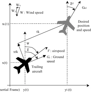
A. Relative position kinematics

In the following, flat non rotating earth is considered as an inertial frame and standard atmosphere is assumed. In addition, and as depicted in Figure 2, the along track distance, denoted tk, is aligned with the trailing aircraft ground speed vector, whereas the cross track distance, denoted xtk, is the right handed positive distance from the trailing to the leading aircraft. Furthermore, χ stands for the track angle of the trailing aircraft, Gs for its groundspeed and V for

its true airspeed. Subscript d is added for all variables related to the desired position : it represents the position and speed of the leading aircraft a few minutes earlier.

Assuming the same wind between the desired and the current position, it can be shown from Figure 2 that the relative motion kinematics between the current and the desired position are governed by the following equations :

(

)

(

)

      − − − +             − =         χ χ χ χ χ χ d sd s d sd G G G xtk tk xtk tk sin cos 0 0 . . & & (1)

American Institute of Aeronautics and Astronautics 3

Furthermore, the relative motion in the vertical plane is the following, where Vz stands for the

vertical speed and γ for the flight path angle :

V V z= zd− ⋅

∆. γ (2)

The track angle χ is the direction followed by the aircraft with respect to the local inertial frame,

whereas the heading angle ψ is the direction

followed by the aircraft with respect to the air as far as the trailing aircraft is supposed to fly in a fully coordinated fashion, i.e. the side-slip angle is always zero. Denoting by ψw the wind direction

from where the wind is blowing (so that ψw is zero

when the wind is blowing from North) and by W its velocity, the following relation holds :

(

)

(

)

   − ⋅ = − ⋅ = π ψ π ψ w y w x W W W W sin cos (3)

Furthermore, groundspeed and track angle are related to airspeed and heading angle through the following relations :

(

)

( )

( )

_{( )}

( )

_{( )}

     ⋅ − ⋅ ⋅ − ⋅ = − ⋅ ⋅ ⋅ − + = w w w s W V W V W V W V G ψ ψ ψ ψ χ ψ ψ cos cos sin sin tan cos 2 2 2 (4) B. Aircraft model

The equations of motion used for the aircraft model are based on three-dimensional point mass differential equations, where V is the true airspeed, z the altitude, ρ(z) the air mass density, m the aircraft mass, T0 the ratio

between engine thrust and air mass density, D0(V,z) the ratio between drag and air mass density, g the acceleration

of gravity, γ the flight path angle, nz the load factor and ψ the heading angle.

( )

₍

_{( )}

₎

_{( )}

(

)

         ⋅ ≈ − = ⋅ − − = ϕ ψ γ γ ρ V g n V g g z V D T m z V z & & & 1 sin , 0 0 (5)

Denoting Cx0 the drag coefficient at zero lift, Cxi the induce drag coefficient and S the reference surface of the

aircraft, the ratio D0(V,z) is computed thanks to the parabolic approximation of the polar curve, where the load factor

has been assumed to remain close to 1. Then :

( )

( )

( )

xi x C z SV mg C SV z V D 2 2 2 0 2 0 2 1 2 1 , ρ + ≈ (6)

The ratio T0 between engine thrust and air mass density, the load factor nz and the bank angle ϕ are considered to

be independent inputs which are adopted as controls.

C. State space representation

Gathering (1), (2) and (5) leads to the following state space representation of the relative guidance dynamics, where u denotes the control vector and x i the state vector:

(

)

(

)

( ) ( )

   ⋅ + = + ⋅ = u x d x c x x x b x u x a x _d 2 2 2 2 2 1 2 1 , , & & (7) Where : y(t) Desired position and speed xtk tk Trailing aircraft χd x(t) xL( t ) yL(t) Gs d V : airspeed ψ χ W : Wind speed Gs : Ground speed (Inertial Frame) Wx Wy

[

]

[

]

[

]

      = = ∆ = T z T T n T u V x z xtk tk x ϕ ψ γ 0 2 1 (8) And :

(

)

(

)

(

(

)

)

                    ⋅ − − − − =           − = V V G G G x x b u x a zd d sd s d sd d γ χ χ χ χ χ χ sin cos , 0 0 0 0 0 0 0 , 2 2 1 & & (9)

It shall be noticed from (4) that groundspeed Gs and track angle χ are function of true airspeed V, heading angle

ψ and wind speed and direction, Vw and ψw respectively.

Furthermore, we have :

( )

( ) ( )

( )

( )

( )

                    =           − ⋅ − ⋅ − = V g V g m z x d V g g m z V D z x c / 0 0 0 / 0 0 0 / 0 / sin / , 2 0 2 ρ γ ρ (10)

In this state space representation, the desired groundspeed Gsd, the desired track angle χd and the desired vertical

speed Vzd are exogenous varying parameters broadcasted through ADS-B. This representation does not take into

account the dynamics of bank angle, load factor and throttle ratio, which are linked to actuators dynamics.

III.

Relative guidance controller

A. Backstepping design

The design objective is to render the equilibrium point (x1=0 ; x2=x2d) globally asymptotically stable. Since the

nonlinear system (7) consists of two state vectors x1 and x2 and taking into account the fact that the matrix a(x2) is

skew-symmetric, the vectorial backstepping technique can be applied by considering this system as two cascaded systems.

In a first step, the virtual control b(x2) is chosen in order to stabilize x1 around 0. The virtual control is chosen as

follows, where Λ1 denotes a positive definite feedback gain matrix (tuning parameter) and z2(x2,x2d) a new state

variable :

(

x2,x2

)

z2

(

x2,x2

)

1x1

b _d = _d −Λ

(11) A candidate Lyapunov function for the x1-system is :

1 1 1 1 2 x x k V ₌ T (12)

Where k1 > 0. Taking into account (11) and the fact that the matrix a(x2) is skew-symmetric, the time derivative

of (12) is :

(

d

)

T T x x z x k x x k V&1=− 1 1Λ1 1+ 1 1 2 2, 2 (13)

We now turn our attention on the z2-system.

In a second step, the dynamics of z2 is computed by time differentiation of (11). Taking into account (7) and

assuming x2d constant leads to :

( ) ( ) ( )

x2

(

c x2 d x2 u

)

z2

(

x2,x2

)

1x1

b ⋅ + ⋅ = & d −Λ &

∇ (14)

A candidate Lyapunov function for the (x1 - z2) system is :

2 2 1 2 2 1 z z V V = + T (15)

American Institute of Aeronautics and Astronautics 5 Denoting

( )

( ) ( )

2 2 2 ˆ b x d x x b

Ld =∇ the Lie derivative of b(x2) along d(x2) and taking into account (14), the time

derivative of (15) is :

( )

( )

(

2 2 1 1

)

2 1 2 V z Lb x L bx u x V c d T & & & _{= + + +Λ} (16)

Taking into account (13) leads to the following :

( )

( )

(

x L bx L b x u

)

z x z k x x k V c d T T T 2 2 1 1 2 1 2 1 1 1 1 1 2=− + + & + + & _{Λ Λ} (17)

For the relative guidance studied in this paper, the matrix

( )

2

x b

∇ has the following expression :

( )

(

(

)

)

( )

( )

          − − = ∇ 0 , 0 , , , 0 , , 2 V V D V z C V B V z A x b γ ψ ψ ψ ψ (18) Where :

(

)

(

)

(

)

(

)

(

)

(

)

(

)

(

)

            − ∂ ∂ − = − ∂ ∂ − = ∂ ∂ − − ∂ ∂ = ∂ ∂ − − ∂ ∂ = χ χ ψ χ ψ χ χ χ ψ ψ χ χ ψ χ ψ χ χ χ ψ d sd d sd s d sd s d sd G V D V G V z C G G V B V G V G V z A cos , cos , , sin , sin , , (19)

The product AD - BC has the dimension of a speed and is given by :

(

χ χ

)

χ ψ ψ χ ₋     ∂ ∂ ⋅ ∂ ∂ − ∂ ∂ ⋅ ∂ ∂ = − d s s sd V G V G G BC AD cos (20)

The partial derivative ∂Gs/∂V, ∂Gs/∂ψ, ∂χ/∂V and ∂χ/∂ψ are computed from (4).

Note : if wind is not considered (i.e. χ=ψ, Gs=V), the above expressions reduce to :

(

)

(

)

(

)

(

)

(

)

(

)

      − − = = − = − = χ χ ψ ψ χ χ ψ ψ d sd d sd G V D V z C G V B V z A cos , 0 , , sin , 1 , , (21) The matrix

( )

( ) ( )

2 2 2 ˆ b x d x x b L_d =∇ is given by :

( )

( ) (

)

(

)

( ) (

)

(

)

( )

                − − = 0 , 0 , , , 0 , , 2 g m z V D V g V z C m z V B V g V z A m z x b Ld γρ ψ ψ ρ ψ ψ ρ (22)

The key point of the control law design is that matrix

( )

2

x b

L_d is invertible. Indeed, we have :

( )

(

)

_{( )(}

_)[

]

(

)

( ) (

)

( ) (

)

(

)

( ) (

)

( ) (

)

( )(

)

                         − − =           − =           − − = − = − 0 / 0 / , , / , / , / , , / , / , 3 2 1 3 2 1 1 2 mV BC AD z c m V z A z mV V B z V V gB c m V z C z mV V D z V V gD c where c c c BC AD z g mV x b L_d ρ ψ ρ ψ γρ ψ ψ ρ ψ γρ ψ ρ (23)

Finally, control vector u is defined in order to regulate the virtual output z2 to zero.

A first alternative is to choose the control vector u as follows, where Λ2 denotes a positive definite feedback gain

matrix (tuning parameter) :

( )

(

)

(

1 1 1 1

( )

2 2 2

)

1 2 k x x Lbx z x b L u=− d ⋅ +Λ + c +Λ − & (24)

So, the time derivative of the candidate Lyapunov function defined by (17) becomes : 2 2 2 1 1 1 1 2 k x x z z V& =− TΛ − TΛ (25)

Hence, the (x1-z2) system is stabilized.

An is sue with the proposed backstepping design is the complexity due to the “explosion of terms” arising from the calculation of the control vector : indeed, the control vector u needs the computation of five terms :

( )

(

)

1 1 1 1

( )

2 1 2 ,k x , x,L bx x b Ld Λ & c − _and 2 2z Λ . In addition, as far as 1

x& is a function of u as stated in the first equation of (7), the expression of the control vector

u given by equation (24) is imp licit : in the case considered in this paper,

1

x& is not measured and consequently the relation shall be manipulated in order to extract u as a function of x1 and x2.

B. Alternative design

An alternative design is developed in order to simplify the expression of the control vector u and to give an explicit formulation of it. This alternative design is based on the Young’s inequality.

Taking into account (11) and the first equation of (7) into (17) leads to :

(

)

(

kI a x u

)

x z

(

z Lb

( )

x L b

( )

x u

)

z x x k V c d T T T 2 2 2 1 2 1 2 1 2 1 1 2 1 1 1 1 2=− Λ + +Λ , −Λ + Λ + + & (26)

Where matrix I stands for identity matrix.

For the specific case studied in this paper, we will assume that matrix Λ1 is diagonal :

{

11 12 13

}

1=diagλ ,λ ,λ

Λ (27)

As a consequence, the expression of

(

(

)

2

)

1 2 1 1I+Λ a x ,u −Λ k is the following :

(

)

(

)

          − − − − = Λ − Λ + 2 13 1 2 12 1 12 11 2 11 1 2 1 2 1 1 0 0 0 0 , λ λ χ λ χ λ λ k k k u x a I k & & (28)

The scalar form of the Young’s inequality is :

0 2 2 1 2+ 2 ∀ > ≤ x dy d d xy (29)

This inequality applied to (28) leads to :

(

)

(

)

1 2 2 2 2 1 1 2 2 2 1 2 1 2 1 2 1 1 2 2 2 2 1 2 , I z x D k x k D z x u x a I k zT T T _      ₊ +     ₊ ≤ − +Λ Λ − Κ Κ (30) Where :                          =           = Κ           − − − = Κ 0 0 0 0 1 0 0 0 1 0 0 0 0 0 0 0 0 0 0 0 0 0 2 11 12 2 2 13 1 2 12 1 2 11 1 1 I k k k χ λ χ λ λ λ λ & & (31)

Parameter k2 is a positive design parameter and matrix D is a design positive diagonal matrix of parameters di :

{

d1,d2,d3

}

diag D= (32) Therefore (26) implies :

( )

( )

(

z Lb x L bx u

)

z z I k D z x k D k x V c d T T T 2 2 2 1 2 2 2 2 1 2 1 2 2 2 2 1 1 1 1 2 2 1 2 2 2  + + +    ₊ +       _{− −} − ≤ Λ Κ Κ − Λ & (33)

American Institute of Aeronautics and Astronautics 7

In order to stabilize the (x1-z2) system, the control vector u is chosen as follows, where Λ2 denotes a positive

definite feedback gain matrix (tuning parameter) :

( )

(

)

(

( ) (

2 1 2

)

2

)

1 2 Lb x z x b L u=− d ⋅ c + Λ +Λ − ₍₃₄₎ Thus (33) becomes : 2 2 2 1 2 2 1 2 2 2 2 1 1 1 1 2 2 1 2 2 2 k I z D z x k D k x V T T     _{− −} −       _{− −} − ≤ Λ Κ Κ Λ − & (35)

The time derivative of the candidate Lyapunov function V2 can be made negative definite for a choice of k1, k2,

Λ1, Λ2 and D such that :

      > − − Λ > Κ − Κ − Λ − 0 2 1 2 0 2 2 2 2 1 2 2 2 2 2 1 1 1 I k D k D k (36)

Finally, the expression of the control vector u according to the initial state variables x1 and x2 is obtained by

taking into account (11) into (34). This leads to :

( )

(

)

(

( )

(

)

(

(

)

)

_   + ⋅ +   + ⋅ − = − d c dbx Lb x x b x x L u 2 1 2 1 1 2 2 1 2 Λ Λ Λ , (37)

The control law (37) is ‘simplified’ compared to (24) in the sense that the time dependant terms

1 1 1

1x and x

k Λ &

have disappear through the bound defined by matrix inequalities (36).

The vector

( )

2

x b

L_c has the following expression :

( )

( ) ( )

( )

          −       ⋅ _{+ ⋅} −           = γ γ ρ _{g C}A m z V D z g x b L_c 0 , sin 0 0 2 (38)

In the following, the matrix Λ2 is chosen as a positive diagonal matrix of parameters λ2i :

{

21 22 23

}

2=diagλ ,λ ,λ Λ (39) So :

(

)

(

(

)

)

(

)

(

(

)

)

(

)

(

(

)

)

(

)(

)

         ⋅ − + ∆ + − + + − − + + = + Λ ⋅ Λ + Λ V V z G xtk G G tk x x b x zd d sd s d sd d γ λ λ λ χ χ λ λ λ χ χ λ λ λ 13 23 13 12 22 12 11 21 11 2 2 1 1 2 1 sin cos , (40)

Parameter k1 has the dimension of sec−2, Λ1 and Λ2 have the dimension of sec−1 and D and k2 have the dimension

of sec.

IV.

Illustrative example

A. Scenario

In this section, a scenario is designed in order to illustrate the properties of the control laws previously designed. The leading aircraft trajectory starts at x0 = 0NM, y0 = 0 NM and FL 100, with initial indicated airspeed of 220

kts and heading of 0 degrees. It is supposed to broadcast its data every second. No wind is considered in this example.

The leading aircraft is assumed to follow a typical arrival procedure, with two turns of 90 degrees. The first turn starts after about 8 min (495 sec) of flight, and the second turn starts after about 10 min (626 sec) of flight. The indicated airspeed decreases firstly towards 180 kts and then towards 140 kts, and the flight level decreases towards 3000 feet after 2 min of flight.

The trailing aircraft trajectory starts at x0 = +10NM, y0 = -7NM and FL 100, with initial indicated airspeed of 225

kts and heading of 330 degrees.

The simulation lasts 15 min (900 sec), and the requested time based separation for the trailing aircraft is constant and equal to 90 sec behind the leading aircraft. The end of simulation is supposed to be the beginning of the final descent.

During the maneuver, the bank angle ϕ, the load factor nz and the indicated airspeed (denoted CAS) of the

    ≤ ≤ ≤ ≤ + ≤ ≤ − kts CAS kts n_z 250 140 06 . 1 94 . 0 . deg 20 . deg 20 ϕ ₍₄₁₎

In addition, longitudinal acceleration is limited to 0.05 × g and roll velocity to 5 deg./sec. In order to take into account the actuator dynamics, bank angle and load factor commands are filtered through a first order low pass filter with a time constant of 1.5 seconds, whereas throttle control is filtered through a first order low pass filter with a time constant of 5 seconds.

Following 9, the drag coefficient at zero lift, denoted Cx0 , the induce drag coefficient, denoted Cxi , the reference

surface of the aircraft, denoted S, and the maximum thrust available have been chosen as follows, which corresponds to a medium range turbojet aircraft :

       = = ⋅ = ⋅ = − − lb level sea at Max Thrust ft S C C xi x 32000 825 10 056 . 6 10 23 . 1 2 2 2 0 (42)

Finally, the values of the constants defining the output vector dynamics have been chosen as follows:

     = = =      = = = − − − − − − 1 23 1 22 1 21 1 13 1 12 1 11 sec 3 . 0 sec 12 . 0 sec 12 . 0 and sec 2 . 0 sec 1 . 0 sec 1 . 0 λ λ λ λ λ λ (43)

Matrix inequalities (36) are satisfied by taking for example k1=0.02 sec−2 and k2=9 sec.

B. Results

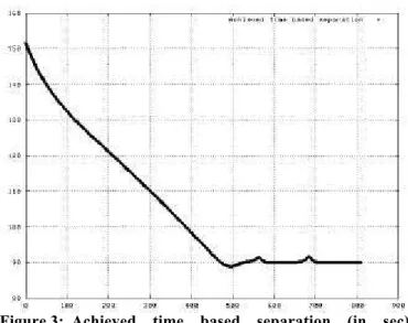
The achieved time based separation between the two aircraft is showed in Figure 3. It has been computed off-line for each position

of the leading aircraft as the difference between the time stamp of the leading aircraft position and the time stamp of the closest trailing aircraft position. As expected, the trailing aircraft moves towards the leading aircraft, with a delay of 90 sec. Moreover, despite two changes of 90 degrees in heading and 40 kts in indicated airspeed (which start after 495 sec of flight), the achieved time based separation remains between -1 sec and +2 sec around the desired delay. The trailing aircraft is stabilized more than 3 minutes (900 - 700 sec) before the end of the simulation.

Figure 4 and Figure 5 show the movements of the leading and trailing aircraft in the horizontal and in the vertical planes. The trailing aircraft makes slight overshoot during the turns, but no

overshoot appears in the altitude tracking. Figure 3: Achieved time based separation (in sec)

American Institute of Aeronautics and Astronautics 9

Figure 6 shows the slant range between the two aircraft. The slant range always exceed 3 NM, which is encouraging from the distance separation standard compatibility point of view.

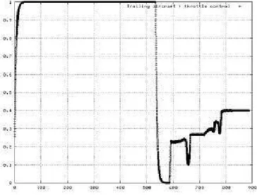
Finally, Figure 7 and Figure 8 show respectively the evolution of the indicated airspeed and throttle control. It appears that the throttle control is quite demanding.

V.

Conclusion

In this paper, the design of a relative guidance controller to automatically move a trailing aircraft towards a leading aircraft and to maintain a constant time delay behind it has been considered. The design considers a 3-D relative motion, including constant wind and lateral, longitudinal and vertical control.

The proposed approach is based on vectorial backstepping. One of the key-point of such a design is the use of a

skew-Figure 4: Leading aircraft and trailing aircraft trajectories in the horizontal plane (orthonormed

axes in NM)

Figure 5: Leading aircraft and trailing aircraft flight levels (FL) versus time (sec)

Figure 6: Actual slant range (in NM) between the two aircraft as a function of time (in sec)

Figure 7: Leading aircraft and trailing aircraft indicated airspeed (kts) versus time (sec)

Figure 8: Throttle control versus time (sec)

Leading aircraft Trailing aircraft Leading aircraft Trailing aircraft Trailing aircraft Runway (not at scale) Leading aircraft

symmetric property of a matrix which appears in the relative motion equations. Furthermore, the design takes advantage of the Young’s inequality to decrease the complexity of the controller due to the “explosion of terms” arising from the calculation of the control vector.

Simulation results based on a typical arrival procedure illustrates the efficiency of the proposed ‘simplified’ backstepping design. Nevertheless, it appears that the throttle control is quite demanding, which may induce an increase in fuel consumption. This deserves further studies in order to smooth this input as well as additional validation in terms of operational scenarios.

Acknowledgments

The authors wish to thank Philippe Louyot and Bernard Hasquenoph from the Centre d’Études de la Navigation Aérienne for their helpful inputs and comments.

References

1

European commission & Eurocontrol, CARA/ASAS Activity 5 description of a first package of GS/AS

applications, version 2.2, september 2002 2

Ivanescu D., Hoffman E., Zeghal K., Impact of ADS-B link characteristics on the performances of in-trail

following aircraft, AIAA GNC Conference, Monterey, USA, August 2002

3 _{Agelii M., Olausson C., Flight deck simu lations of station keeping, ATM 2001 R&D seminar, Santa Fe, paper}

no. 17

4 _{Vanken P., Hoffman E., Zeghal K., Influence of speed and altitude profile on the dynamics of in-trail following} aircraft, AIAA GNC Conference. Denver, Colorado, August 2000, Paper No. 2000-4362

5

Miquel T., Mora-Camino F., Levine J., Aircraft relative guidance: a flatness synthesis of a new autopilot mode , 5th USA/Europe Air Traffic Management R&D Seminar, Budapest, Hungary, June 2003

6

Miquel T., Mora -Camino F., Achaibou K., A feedback linearizing controller for relative guidance between

commercial aircraft, AIAA GNC Conference. Austin, Texas, USA, August 2003, Paper No. 2003-5410 7

Hoffman E., Ivanescu D., Shaw C., Zeghal K., Analysis of constant time delay airborne spacing between

aircraft of mixed types in varying wind conditions, 5th USA/Europe Air Traffic Management R&D Seminar, Budapest, Hungary, June 2003

8

Krstic M., Kanellakopoulos I., Kokotovic P.V., Nonlinear and Adaptative Control Design, John Wiley & Sons Ltd, New York, 1995