Study on the Homogenization Speed in a Tank Equipped with Maxblend Impeller

(1)

UNIVERSITÉ DE MONTRÉAL

STUDY ON THE HOMOGENIZATION SPEED IN A TANK EQUIPPED WITH

MAXBLEND IMPELLER

MARYAM HASHEM

DÉPARTMENT DE GÉNIE CHIMIQUE ÉCOLE POLYTECHNIQUE DE MONTRÉAL

MÉMOIRE PRÉSENTÉ EN VUE DE L’OBTENTION DU DIPLÔME DE MAÎTRISE ÈS SCIENCES APPLIQUÉES

(GÉNIE CHIMIQUE) JUIN 2012

(2)

UNIVERSITÉ DE MONTRÉAL

ÉCOLE POLYTECHNIQUE DE MONTRÉAL

Ce mémoire intitulé:

STUDY ON THE HOMOGENIZATION SPEED IN A TANK EQUIPPED WITH MAXBLEND IMPELLER

présenté par: HASHEM Maryam

en vue de l’obtention du diplôme de : Maîtrise ès sciences appliquées a été dûment accepté par le jury d’examen constitué de :

M. HENRY Olivier, Ph.D, président

M. FRADETTE Louis, Ph.D, membre et directeur de recherche M. VIRGILIO Nick, Ph.D, membre

(3)

DEDICATION

(4)

ACKNOWLEDGEMENTS

First of all, it is with immense gratitude that I acknowledge the support and help of my supervisor Professor Louis Fradette. I sincerely thank him for accepting me in his research group, his kind guidance, helpful suggestions, encouragement and confidence in me.

I would like to thank my committee members, Professor Nick Virgillio and Professor Olivier Henry.

Special thanks to Mr. Daniel Dumas and Mr. Jean Huard for their helps and technical support. I would like to thank all members of URPEI group; my friends and my colleagues for their great attitude.

I would like to thank my parents, and my husband for their patience, unconditional love, and encouragements. This work was not possible without their presence.

(5)

RÉSUMÉ

Le but de ce travail est de caractériser expérimentalement la performance du mélangeur Maxblend dans le cas de suspensions solides.

De par le très grand nombre d’applications industrielles qui utilisent le mélange solide-liquide, d'importants efforts ont été mis en œuvre pour améliorer la compréhension de cette opération. Le principal objectif du mélange solide-liquide est de créer et de maintenir l'homogénéisation de la suspension. De telles opérations étant généralement réalisées dans des cuves agitées mécaniquement, le choix d'un agitateur à haute performance est primordial pour assurer à la fois la dispersion des particules et leur suspension.

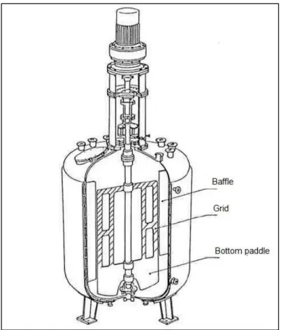
L'agitateur Maxblend est un des plus efficaces parmi la nouvelle génération de mélangeur. Il est composé d’une large pale, située au bas de la cuve, et d'une grille sur la partie supérieure. La pale joue le rôle d'une pompe et la grille permet de créer la dispersion. Le mélangeur Maxblend est une alternative intéressante aux agitateurs raclant et est utilisé dans différents procédés, allant de la dispersion de gaz à la polymérisation.

Dans ce travail, une étude expérimentale a été réalisée pour caractériser la performance d’un système de mélange équipé d’un agitateur Maxblend et d’une cuve cylindrique, dans le cas des fluides newtoniens.

La vitesse d'homogénéisation (NH), correspondant à la vitesse critique pour obtenir une

suspension uniforme, est mesurée par tomographie à résistance électrique. Le travail expérimental a permis d’obtenir, pour diverses viscosités de fluides, la puissance consommée et le temps de mélange. De plus, l’impact de la géométrie de la cuve, de l'espace entre le fond de la cuve et l'agitateur, ainsi que la quantité de solide sur l’efficacité de l’agitateur à générer la suspension ont été étudiés. En se basant sur ces résultats, il est possible de confirmer que le Maxblend est un mélangeur performant, puisqu’il permet d’obtenir une suspension uniforme, un temps de mélange court avec une faible consommation d'énergie.

Mots clé: Mélange, Suspension, Solide-Liquide, Maxblend, Newtonien, fluide visqueux,

(6)

ABSTRACT

The goal of this work is to characterize experimentally the performance of a Maxblend impeller for solid suspensions.

Significant efforts have been devoted to better understand the solid liquid mixing phenomena, because of the large number of industrial applications of this operation. The major objective of solid-liquid mixing is to first create and then maintain homogenous slurry conditions. Such operations are commonly carried out in tanks stirred by suitable mechanical agitators. The important point in designing a solid-liquid suspension is choosing a high performance impeller for achieving both the dispersion of the particles and their suspension, at the same time.

The Maxblend impeller is one of the most efficient kinds of the new generation impellers. It is composed of a large bottom paddle and an upper grid. The paddle acts as a pump and the grid provides dispersion capabilities. The Maxblend impeller represents an interesting alternative to close clearance impellers and it has been used in many different processes ranging from gas dispersion to polymerizations.

In this study, an experimental investigation is carried out to characterize the mixing performance, for Newtonian fluids in a cylindrical tank equipped with a Maxblend impeller.

The homogenization speed (NH) is introduced as the critical speed for the uniform suspension and

it is measured by Electrical Resistance Tomography. The experimental work consisted in obtaining the power consumption and the mixing time for various liquid viscosities in Maxblend. Also the effects of vessel geometry, off-bottom clearance and solid loading on solid suspension efficiency are investigated. According to the results, it can be confirmed that Maxblend is an interesting technology to obtain a uniform suspension in light of short mixing time and low power consumption.

Key Words: Mixing, Suspension, Solid-Liquid, Maxblend, Newtonian, Viscous fluid, Homogeneous

(7)

LIST OF FIGURES

Figure 1: Maxblend reactor……….……….. 3

Figure 2: Mixing mechanism... 4

Figure 3: Range of Maxblend impeller efficiency………. 4

Figure 1-1: Degrees of suspension. (a) Partial suspension, (b) Complete suspension, (c) Uniform suspension………... 7

Figure 1-2: Distributive mixing versus dispersive mixing……….... 8

Figure 1-3: Power curve for solid suspension in compare with single phase……… 22

Figure 1-4: Radial and axial flow pattern... 23

Figure 1-5: Ungassed power number of impellers in turbulent regime for different impellers… 25 Figure 1-6: Schematic of the Maxblend impeller... 28

Figure 1-7: Concept of the Maxblend design... 29

Figure 1-8: Effect of Reynolds numbers on flow pattern and velocity field for un baffled configuration: (a) Re = 80 (b) Re = 40... 30

Figure 1-9: (a) Straight Maxblend impeller (b) Wedge Maxblend impeller... 30

Figure 1-10: Maxblend modified (a) N◦1 and (b) N◦2... 31

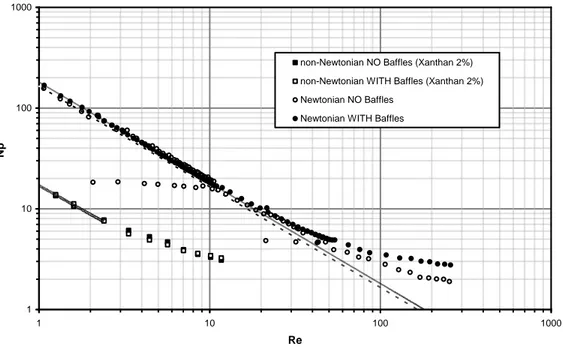
Figure 1-11: Power curves for Newtonian and non-Newtonian fluids, Maxblend 35 L... 32

Figure 1-12: Comparison of various mixing agitators based on the dimensionless time... 32

Figure 1-13: Comparison of various mixing geometries based on the mixing energy versus the Re mixing time. Data for agitators other than Maxblend were taken from Yamamoto et al., 1998………... 33

Figure 1-14: The schematic of ERT system... 36

Figure 1-15: Schematic diagram of electrode arrangement and placement... 38

Figure 1-16: Tomogram showing region of high and low conductivity... 39

Figure 1-17: Tomograms of relative conductivity. (a) 40th frame, (b) 50th frame, (c) 60th frame, (d) 70th frame, (e) 80th frame, (f) 90th frame, (g) 100th frame, (h) 110th frame... 40

Figure 2-1: Schematic of the mixing rig... 44

Figure 2-2: Wedge Maxblend impeller (a) Flat bottom and (b) Dish bottom... 45

(10)

Figure 2-4: The schematic of ERT system... 49

Figure 2-5: Typical suspending evolution curve (Tap water, ν=5 wt%)... 51

Figure 2-6: Reproducibility experiments, N=100 rpm (Tap water, ν=5 wt%)... 52

Figure 2-7: Reproducibility experiments, N=60 rpm (Tap water, ν=5 wt%)... 53

Figure 2-8: Conductivity curve at 60 rpm impeller speed (µ=0.1 Pa.s, ν=5 wt%)... 53

Figure 2-9: Conductivity curve for different impeller speed (µ=0.1 Pa.s, ν=5 wt%)... 54

Figure 3-1: Solid suspending evolution with Maxblend... 55

Figure 3-2: Tomograms obtained for the solid suspension at μ= 0.1 Pa.s, ν=5 wt%, dp=500µm: (a) N=40 rpm, (b) N=53rpm... 56

Figure 3-3: Normalized average conductivity curve for the solid suspension at μ= 0.1 Pa.s, ν=5 wt%, dp=500µm, NH=53rpm... 57

Figure 3-4: Power curves for single phase and solid suspension (Glucose- water solution and glass beads)... 58

Figure 3-5: Experimental mixing times for a single fluid (Glucose- water solution) and with solids present (5 wt%)... 59

Figure 3-6: The effect of bottom geometry on NH (glucose-water solution, µ= 4.78 Pa.s , ν=5-25 wt%)... 61

Figure 3-7: Power curves for 5wt% solid suspension in flat and dish bottomed tank... 61

Figure 3-8: Effect of bottom clearance on the NH (Tap water and glass beads, ν=5 wt%)... 62

Figure 3-9: Effect of solid concentration on NH (glucose-water solution, µ= 4.78 Pa.s, 58<Re<83)... 63

Figure 3-10: Effect of liquid viscosity on NH (glucose-water solution and glass beads, ν=5 wt%)... 64

Figure 3-11: Homogenization speed curve (glucose-water solution and glass beads, ν=5 wt%) ... 65

Figure 3-12: Sampling measurement system (SHI Mechanical & Equipment, 2011)... 66

Figure 3-13: Comparison of ERT with Sampling technique (Tap water and glass beads, ν=5 wt%)... 67

(11)

LIST OF TABLES

Table 1: Applications of Maxblend mixer...5

Table 1-1: Hydrodynamic regimes for settling particles ...11

Table 1-2: Values of the exponent in Maude empirical correlation...12

Table 2-1: Geometrical details of Maxblend systems...45

Table 2-2: Specification of solid particles...47

(12)

LIST OF SYBOLS

C Off-bottom clearance (m)

CD Drag coefficient

CH Cloud height (m)

dp Particle size (m)

(dp)43 Mass-mean particle diameter (m)

D Impeller diameter (m)

Fr Froude number

gc Acceleration of gravity (m.s-2)

H Liquid depth in the stirred tank (m)

Hi Impeller clearance (m)

Kp Power constant

Kp(n) Power constant (for non Newtonian fluids)

Ks Shear rate constant

M Flow consistency index (Pa.sn)

M Torque (N·m)

Mc Corrected torque (N·m)

Mm Measured torque (N·m)

Mr Residual torque (N·m)

N Power-law index

N Impeller rotational speed (rps)

NH Homogenization speed

Njs Impeller speed for just-suspended (rps)

Np Power number

N*p Modified power number

P Power consumption (W)

Re Reynolds number

Re p Particle Reynolds number

(13)

Re imp Impeller Reynolds number

Re* Modified Reynolds number

S Zwietering constant T Tank diameter (m) Tm Mixing time V Voltage difference Vt Settling velocity (m.s-1) Vts Hindered velocity (m.s-1)

X Mass ratio of suspended solids to liquid (kg solid/kg liquid)

Z Liquid depth in vessel (m)

Greek Letters Ρ Density (kg.m-3) ρl Liquid density (kg.m-3) ρs Solid density (kg.m-3) ρ* Suspension density (kg.m-3) µ Viscosity (Pa·s)

µl Liquid viscosity (Pa·s)

µo Viscosity of continuous phase (Pa·s)

µr Relative viscosity (Pa·s)

µ* Suspension viscosity (Pa·s)

Ν Kinematic viscosity of the liquid (m2.s-1)

Apparent viscosity of non Newtonian fluid (Pa·s)

Ψ Sphericity

Ø Volume fraction of solids in suspension (wt%)

φv Solid volume concentration (wt%)

(14)

Abbreviations

A100, A200, A310, A320 Lightnin

ERT Electrical resistance tomography

CBT Concave Blade Turbine

DT (n) Disk turbine (number of blades)

HE-3 High efficiency

HF-4 4-bladed Hydrofoil

PBT-D (n) Pitched blade turbine down pumping flow (number of blades)

PBT-U (n) Pitched blade turbine up pumping flow (number of blades)

RT (n) Rushton turbine (number of blades)

vol% Volume percent

(15)

INTRODUCTION

Mixing processes are encountered widely throughout industry involving chemical and physical changes (Paul et al., 2004). Mixing is a central feature of many processes in the polymer processing, petrochemicals, biotechnology, pharmaceuticals, pulp and paper, coating, paints and automotive finishes, cosmetics and consumer products, food, drinking water and wastewater treatment, mineral processing, fine chemicals and agrichemicals, etc.

Despite the extensive applications of mixing, tremendous problems are very often encountered in industries due to a lack of understanding of the fundamentals involved in mixing processes. When viewed on an international scale, the financial investment in costs of mixing processes is considerable (Nienow et al., 1997). Process objectives are crucial to the successful manufacturing of a product. If scale-up fails to produce the required product yield, quality, the costs of manufacturing may be increased significantly, and perhaps more importantly, marketing of the product may be delayed or even cancelled in view of the cost and time required to correct the mixing problem (Paul et al., 2004).

It has been estimated that 1-10 billion dollars/year are lost by North American industries due to mixing problems (Paul et al., 2004). Most industries are suffering from an oversimplified design of the mixing systems. While an oversimplified design leads to low quality products, an overly complex design is extremely costly in large scale production plants.

Although extensive experimental and numerical studies have been done on mixing systems, the successful design, operation, and scale-up of such systems still present a challenge.

Among the various mixing processes (e.g., liquid-liquid, gas-liquid, solid-liquid), solid-liquid mixing is one of the most important mixing operations, because it plays a crucial role in many unit operations, such as suspension polymerization, solid-catalytic reaction, dispersion of solids, dissolution and leaching, crystallization and precipitation, adsorption, desorption, and ion exchange (Paul et al., 2004, Zlokarnik, 2001). The major objective of solid-liquid mixing is to create and maintain homogeneity in a slurry, or to improve the rate of mass and heat transfer between the solid and liquid phases.

With this objective in mind, researchers across the world have started to study and design high performance mixing setups for solid-liquid mixing.

(16)

For low viscosity fluids the most common mixing systems are based on high speed blade turbines such as flat blade turbine, pitched blade turbine and hydrofoils in tanks equipped with baffles. In high viscosity fluids these turbines lose their efficiency because of the high clearance, dead zones and cavern effects. In order to alleviate these problems, close clearance impellers such as helical ribbon, anchor, or Paravisc rotating at low speeds could be used. These impellers provide more efficient top to bottom flow, and thus good homogenization. In solid liquid mixing of high viscosity continuous phases, usually two mechanisms are required: the first is used to reduce average particle size and the second to reach a uniform degree of dispersion throughout the vessel. A combination of the impellers mentioned above can achieve this task, resulting in the integration of several mixing step within one vessel. Multi shaft mixers can be used to carry out mixing in highly viscous systems. In many mixing processes, the rheological properties of the mixture evolve during the mixing operation. The rheology modification often originates from a chemical reaction, additives, or physical change in the solution structure. The viscosity of the final product is often higher than that of the starting material. Non-Newtonian properties may develop, depending on the nature of the reactants involved in the process. Specific types of agitators are suitable for such processes. Indeed, it is uncommon to change agitators during the reaction. Mixing specialists look for versatile agitators that can fulfill the requirements of these processes while handling the variable rheological properties.

To meet the needs of these processes with variable rheological properties a new impeller design called Maxblend has been proposed by Sumitomo Heavy Industries, Japan. It belongs to the family of the so-called “wide” impellers and has been recently introduced for the chemical process industries (See Figure 1). This impeller is mounted in a vessel with a very small clearance between the bottom wall and the lower edge of the impeller. Baffles at the vessel wall can also be installed depending on the flow regime and application in mind. The impeller’s main advantages are a precise control of the mixing flow in the vessel and the generation of a relatively uniform shear contrary to open turbines, where high shears are located in the vicinity of the turbine, yielding cavern phenomena when shear-thinning fluids are used (Solomon et al., 1981).

(17)

Figure 1: Maxblend reactor (SHI Mechanical & Equipment, 2001)

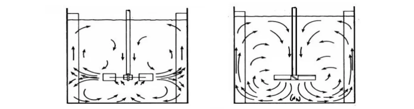
The mixing mechanism operated by the Maxblend is illustrated in Figure 2. The top to bottom pumping induced by the Maxblend is remarkable, the flow goes upward near the wall and downward in the center along the shaft.

This impeller is effective over a wide range of viscosities (Figure 3). It would therefore retain a high mixing efficiency for many processes, regardless of viscosity changes during mixing.

(18)

Figure 2: Mixing mechanism (SHI Mechanical & Equipment, 2001)

Figure 3: Range of Maxblend impeller efficiency (SHI Mechanical & Equipment, 2001)

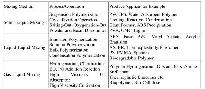
SHI uses the Maxblend for a variety of applications in liquid-liquid, liquid-solid and gas-liquid mixing. According to the manufacturer claims, the Maxblend can handle processes from suspension polymerization and crystallization operation to high viscosity gas absorption (Table 1).

(19)

Table 1: Applications of Maxblend mixer

Mixing Medium Process/Operation Product/Application Example

Solid -Liquid Mixing

Suspension Polymerization Crystallization Operation Salting-Out, Oxygenation-Out Powder and Resin Dissolution

PVC, PS, Water Adsorbent Polymer Cooling, Reaction, Condensation Clam Former, ABS Precipitation PVA, CMC, Lignin Liquid-Liquid Mixing Emulsion Polymerization Solution Polymerization Bulk Polymerization Condensation Polymerization

ABS, Paste PVC, Vinyl Acetate, Acrylic Emulsion

AS, BR, Thermoplasticity Elastomer PS, PMMA, Spandex

Biodegradable Polymer Gas-Liquid Mixing

Hydrogenation, Chlorination EO, PO Addition Reaction

High Viscosity Gas

Absorption

High Viscosity Cultivation

Polymer Hydrogenation, Oils and Fats, Amine Surfactant

Thermoplastic Elastomer etc. Biopolymer, Bio-Cellulose

Although these claims make this impeller pretty attractive for solid-liquid mixing applications, in practice, the actual performance of the impeller is not well documented. The objective of this work is to describe the solid-liquid mixing behavior when using a Maxblend. The project considers Newtonian viscous mixing. We are especially interested in the performance characteristics of this impeller and how they compare when the impeller operates in different operating and design conditions. The study is performed experimentally.

(20)

CHAPTER 1 LITERATURE REVIEW

1.1. Solid Suspension

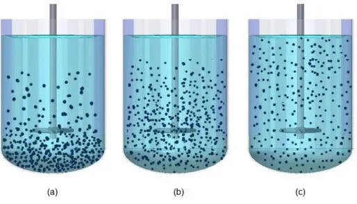
Dispersion generally consists of discrete particles randomly distributed in a fluid medium. Dispersion can be divided into three categories: solid particles in a liquid medium (suspension), liquid droplets in a liquid medium (emulsion) or gas bubbles in a liquid (foam). Suspension is the dispersion of particulate solids in a continuous liquid phase, which is sufficiently fluid to easily circulate by a mixing device (Uhl and Gray, 1986). However, in the case that a system incorporates powders and fine particles throughout the liquid medium is considered as dispersion or colloidal suspension (Harnby et al., 1997). When the particle concentration and, for a range of sizes, the size distribution is constant throughout the tank, homogeneous suspension exists (Harnby et al., 1997). The quality of solid suspension can be divided into three regimes: on-bottom (partial), off–on-bottom (complete) and homogeneous (uniform) suspension regimes (Paul et al., 2004). These are illustrated in Figure 1-1.

On-bottom motion or partial suspension: This situation can be described as the complete

motion of all solid particles in the whole tank, regardless of aggregation of particles in corners or other parts of the tank bottom, which means there are still some particles in motion that have contact with the tank bottom. In this case, not all the surface area of particles is available for chemical reaction or mass or heat transfer. This condition is sufficient for the dissolution of solids with high solubility.

Off-bottom or complete suspension: This situation can be described as the complete motion of

particles where no particle lays on the tank bottom for more than 1 to 2 seconds, even though the suspension throughout the tank might not be uniform. Due to this whole motion, the surface area reaches the maximum level for the chemical reaction and diversity of transfer. Since this situation

(21)

is the minimum mixing requirement in most solid-liquid systems, the “just suspended speed” is always chosen as an important parameter in the study of the solid-liquid system.

Uniform suspension: This situation can be described as the formation of both uniform particle

concentration and particle size distribution in the whole tank. Any further increase in impeller speed or power does not appreciably improve the solids distribution. This condition is required for crystallization and solid catalyzed reaction.

Suspension percentage,

(1-1)

might be greater than, equal to, or smaller than 100%. As for the uniform suspension, the suspension percentage is 100%. Basically, by increasing the power input or rotating speed, the particle distribution does not obviously improve. This suspension is required in processes, such as the crystallization process and solid catalyzed reaction, where uniform solids concentration is vital to the efficiency of an operation unit or even the continuity of a whole production line. Of course, this ideal scenario is based on more power input, more effective equipment configuration, and certain operating conditions.

Figure 1-1: Degrees of suspension. (a) Partial suspension, (b) Complete suspension, (c) Uniform suspension (Tahvildarian et al., 2011)

(22)

Distribution and dispersion are discussed when the quality of solid-liquid mixing is studied. The uniform suspension depends on both good distribution and dispersion. Figure 1-2 presents examples to clarify the difference between distribution and dispersion. In the first row, aggregations exist in both conditions. In Figure (a), the particles aggregate randomly resulting in a bad distribution and a bad dispersion. In (b), aggregations distribute orderly which is considered as a good distribution and a bad dispersion. Figure (c) demonstrates a good dispersion and a bad distribution where there are still some aggregations from a microscopic perspective, but for each aggregation, the distribution of particles is uniform. Finally in (d), there is no aggregation and particles distribute uniformly within the tank in what is called uniform suspension.

Figure 1-2: Distributive mixing versus dispersive mixing

The physical and chemical properties of liquid and solid particles influence the fluid-particle hydrodynamics and, consequently, the suspension. For example, large, dense solids are more difficult to suspend than small particles with low density in the same continued phase. Another

(23)

example is spherical particles, which are more difficult to suspend than thin flat disks (Paul et al., 2004). The properties of both the solid particles and the suspending fluids influence the suspension. Also vessel geometry and agitation parameters are important. The important liquid and solid properties and operational parameters are as follows:

a) Physical properties of the continuous phase:

 Liquid density, ρl

 Density differences, ρs-ρl  Liquid viscosity, µl

b) Physical properties of solid particles:

 Solid density, ρs  Particle size, dp

 Particle shape or sphericity

 Wetting characteristics of the solid

 Tendency to entrap air or head space gas

 Agglomerating tendencies of the solid

 Hardness and friability characteristics of the solid c) Process operating conditions:

 Liquid depth in vessel

 Solids concentration d) Geometric parameters:

 Vessel diameter

 Bottom head geometry: flat, dished, or cone-shaped

 Impeller type and geometry

 Impeller diameter

 Impeller clearance from the bottom of the vessel

 Baffle type, geometry, and number of baffles e) Agitation conditions:

 Impeller speed, N

(24)

For example, for small solid particles, which have a density approximately equal to the liquid, once suspended they continue to move with the liquid. The suspension behaves like a single-phase liquid at low solid concentrations. For solid particles with higher density their velocities are different from that of the liquid. The drag force on the solid particles caused by the liquid motion must be sufficient and directed upward to counteract the tendency of the particles to settle by the gravity force.

Solid suspension processes consume a huge amount of processing time and energy, so it is necessary to know about the various factors affecting them. There are some studies investigating these parameters such as the following:

a) Physical properties of liquid, such as density and viscosity (Chapman et al., 1983, Ibrahim and Nienow, 1994).

b) Physical properties of solid, such as density, particle size, sphericity, wetting characteristics of solid, agglomerating tendencies of the solid and hardness and friability characteristics of the solid (Altway et al., 2001, Ayranci and Kresta, 2011).

c) Process operating conditions, such as liquid depth in the vessel and solid concentration (Einenkel, 1980).

d) Geometric parameters, such as vessel diameter, bottom head geometry like flat, dished or cone-shaped, impeller type and geometry, impeller diameter, impeller clearance from the bottom of the vessel, baffle type and the geometry and number of baffles (Biswas et al., 1999, Wu et al., 2001).

e) Agitation conditions, such as impeller speed, impeller power, impeller tip speed, level of suspension achieved and liquid flow pattern (Biswas et al., 1999).

1.1.1. Settling Velocity

When a dense solid particle is placed in a motionless fluid, it will accelerate to a steady-state settling velocity, which is called the free settling velocity. It occurs when the drag forces balance the buoyant and gravitational forces of the fluid on the particle. However, in equilibrium the sum of these forces is zero.

(25)

In Newtonian fluids for spherical particles, the free settling velocity (vt) is a function of different

physical and geometrical parameters and it is defined by

(1-2)

In this equation, CD is the drag coefficient, which directly depends on the particle Reynolds

number (Rep),

(1-3)

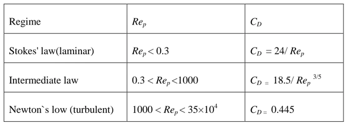
and particle shape. The expression of the drag coefficient for each flow regimeis defined in Table 1-1. By substituting each definition of drag coefficient in equation 1-2, the terminal velocity for each regime, in the case of low concentration suspensions, could be calculated (Paul et al., 2004).

Table 1-1: Hydrodynamic regimes for settling particles (Paul et al., 2004)

Regime Rep CD

Stokes' law(laminar) Rep < 0.3 CD = 24/ Rep

Intermediate law 0.3 < Rep <1000 CD = 18.5/ Rep

3/5

Newton`s low (turbulent) 1000 < Rep < 35×10

4

CD = 0.445

1.1.2. Hindered Settling

In the case of low concentration suspensions, the settling velocity can be evaluated using equation 1-2. However, when the concentration is increased (>2%) particle-particle interactions become significant and other particles decrease the value of Vt (Blanc and Guyon, 1991).

(26)

upward flow of fluid created by the downward settling of particles, or increase in the apparent suspension viscosity and density. An empirical correlation for hindered settling velocity is reported by Maude as

, (1-4)

where Vts is the hindered settling velocity, Vt is the settling velocity, Ø is the volume fraction of

solids in suspension, and n is a function of the particle Reynolds number (Rep) which is defined

as follows (Maude and Whitmore, 1958):

Table 1-2: Values of the exponent in Maude empirical correlation

Rep < 0.3 n = 4.65

0.3< Rep <1000 n = 4.375 Rep -0.0875

1000< Rep n = 2.33

This expression is recommended for preliminary estimates of the effect of solid concentration on settling velocity (Paul et al., 2004).

1.1.3. Rheological Properties of Suspension

Rheology is the science of flow and deformation of materials. The rheology of suspensions is an important subject in the field of rheology since it shows various types of rheological characteristics, such as thixotropy, shear thinning, shear thicking, viscoelastic, etc. We need to develop our knowledge about suspension rheology for a wide range of industrial applications, such as paint, ink, cement, cosmetics, food, and agricultural products in order to select the best production conditions for the specific application.

The viscosity of slurry is a function of the continuous phase viscosity, particle-particle interactions, and the size distribution, concentration, and the shape of particles. It is also a

(27)

function of the shear rate, and can be a function of the shearing time (Shamlou, 1993). Suspensions are classified depending on the rheological behaviour of the continuous phase (Jinescu, 1974).

a) Suspension in a Continuous Newtonian Phase b) Suspension in a Continuous Non-Newtonian Phase

In Newtonian continuous phase, Newtonian behavior is observed for small solid concentrations, whereas the suspension is usually non-Newtonian for high solid concentration (Shamlou, 1993). For non Newtonian medium, a suspension shows non-Newtonian behaviour even with small concentrations of solid particles. In small solid particle concentrations, the non-Newtonian behaviour is caused by the continuous phase. However, with high concentrations of solid particles, particle-particle interactions usually heighten the non-Newtonian behaviour of the suspensions.

For non-Newtonian shear thinning liquids, higher agitator speeds can be expected than for Newtonian liquids, especially where a single impeller is used. This is due to the rapid fall-off in fluid motion away from the impeller. Hence for very shear thinning fluids a multi impeller is recommended; also large diameter impellers are more effective at creating movement at the liquid surface than small impellers and so are more effective at drawing solids into the liquid (Shamlou, 1993).

Many experimental and theoretical works have been carried out to predict the rheological behaviour of suspensions. These models were derived under the assumption of spherical, rigid and mono-dispersed particles.

For example, for the viscosity of suspension, which contains a volume concentration of spherical solid particles up to 50%, Gillies et al. derived an equation, which is in good agreement with experimental results (Gillies et al., 1999):

(1-5)

where µr is relative viscosity, φ is the volume fraction of the spheres. In this equation the terms of

an order of two and higher are a result of particle-particle interactions in highly concentrated suspensions.

(28)

1.2. Solid-Liquid Suspension in Mechanically Agitated Vessels

1.2.1. Hydrodynamic Regimes

Suspension of solid particles needs the input of mechanical energy into the solid-liquid system by some mode of agitation. The input energy makes a turbulent flow field in which solid particles are lifted from the base of vessel and then dispersed and distributed throughout the liquid.

Nienow discussed in some detail the complex hydrodynamic interactions between solid particles and fluids in mechanically agitated tanks. First, there is a drag force on particles arising from the boundary layer flow across the bottom of the tank. To suspend the particle the velocity of the boundary layer flow should be ten times greater than the particle settling velocity in a motionless fluid. Second, turbulence breaks the boundary layer and if the frequency and energy levels are high enough, a suspension will be started (Nienow et al., 1997). Latest measurements of the 3D velocity of both the solid particles and the fluid confirm this complexity (Paul et al., 2004). Solids pickup from the tank bottom is achieved by a combination of the drag and lift forces of the moving fluid on the solid particles and the bursts of turbulent eddies originating from the bulk flow in the tank. Among the various models which explain the hydrodynamics of solid-liquid suspensions, the most successful one was proposed by Baldi et al.. According to his model, the particles in the vessel base are suspended mainly due to turbulent eddies of approximately the same scale as the particle size (Baldi et al., 1978).

1.2.2. Solid-liquid Dispersion in High Viscous Continuous Phase

When the continuous phase viscosity is considered to be low enough to reach a turbulent regime, obtaining a uniform suspension is a difficult task due to the high settling velocity of the particles. In most industries dealing with food, polymer, pharmaceutical and biotechnological processing, mixing involves high viscosity medium or low rotating speeds, which means operating at the laminar regime.

(29)

Processing these high viscosity materials may require the incorporation of fine solids. To achieve a solid dispersion in a viscous continuous phase, the objective is to produce a uniform material with an acceptably low level of agglomerates of the basic individual particles.

In high viscosity continuous phases, in the absence of turbulent eddies, the stresses, which are produced within the liquid during laminar flow, are responsible for breaking and rupturing agglomerates of particles and dispersing them uniformly as individual particles throughout the vessel. In the absence of molecular diffusion, this mechanism tends to reduce the size and scale of the unmixed clumps. High shear stresses for such a task can be achieved in mixers which provide high shear and the components should pass through these zones as often as possible. In mixers handling high viscosity fluids (such as Rneaders, internal mixers, planetary mixers, and helical ribbons) the flow patterns are very complex. All of these mixers incorporate high shear zones and regions where fluids are redistributed. The shear produced, however, in the high shear zones of these mixers may not be enough to reduce the size of the agglomerates and break the lumps as required. In this case, incorporation of a high shear mixer and a distributive mixer for high viscosity continuous phases would improve the mixture quality.

1.2.3. Just Suspension Speed in Stirred Tanks (N

js

)

The minimum impeller speed at which all the particles reach complete suspension is known as

Njs. Under this condition, the maximum surface area of the particles is exposed to the fluid for

chemical reaction or mass or heat transfer. The “just suspended” situation refers to the minimum agitation conditions at which all particles reach complete suspension.

Many efforts have been made to characterize this parameter experimentally, and theoretically which result in different equations for predicting it.

One of the first studies in this field was done by Zwietering (Zwietering, 1958). He introduced the visual observation method to find out Njs. The motion of the solid particles on the tank bottom

was visually observed through the transparent tank. Njs was measured as the speed at which no

solids are visually observed to remain at rest on the tank bottom for more than 1 or 2 seconds. Simplicity is the main advantage of visual methods. However, only with careful and experienced observation it is possible to achieve ±5% reproducibility in a diluted suspension. Furthermore,

(30)

visual methods need a transparent vessel, which is feasible for most laboratory-scale studies, but rather out of reach for large-scale tanks. To overcome the limitations of the visual method other techniques have been proposed and different concepts have been applied, like solid concentration change directly above the vessel bottom (Bourne and Sharma, 1974a, Musil and Vlk, 1978), ultrasonic beam reflection from the static layer of the solid on the vessel base (Buurman et al., 1986), variation of power consumption or mixing time (Rewatkar et al., 1991), pressure change at the bottom of the vessel (Micale et al., 2000, Micale et al., 2002).

Experimental techniques have been used to perform many empirical and semi-empirical investigations on solid suspension, results of which have been critically reviewed in the literature (Armenante and Nagamine, 1998, Armenante et al., 1998, Paul et al., 2004, Harnby et al., 1997). Most presented correlations have been developed based on the visual technique. Most of the studies resulted in modifications of model parameters in the Zwietering correlation. Zwietering derived the following correlation from dimensional analysis. He estimated the exponent by fitting the data to the just-suspended impeller speed (Zwietering, 1958),

(1-6) where: _(1-7) (1-8) (1-9)

where D is the impeller diameter, dp is the mass-mean particle diameter (dp)43, X is the mass ratio

of suspended solids to liquid × 100, S is the dimensionless number which is a function of impeller type, ν is the kinematic viscosity of the liquid, gc is the gravitational acceleration constant, and ρs

and ρl are the density of particle and the density of liquid, respectively.

He showed that in the calculation of Njs a significant variance appears and there is no correlation

(31)

the reported values were in the range of -56% to +250% from their own value. Different empirical correlations have been developed based on experimental characterization of Njs.

Prediction of Njs was a subject of few CFD studies (Fletcher and Brown, 2009, Lea, 2009,

Murthy et al., 2007, Panneerselvam et al., 2008). Kee and Tan presented CFD approach for predicting Njs and characterized effect of D/T and C/T on Njs (Kee and Tan, 2002).

1.2.4. Cloud Height

In solid suspension, there is a distinct level at which most of the solids become lifted within the fluid. This height of the interface from the bottom of vessel is called cloud height and above this interface there are only a few solid particles. Liquid below this height, however, is solid-rich (Bittorf and Kresta, 2003). Measurement of cloud height within the stirred vessel provides a qualitative indication of suspension quality. Many studies have been done to express homogeneity as a function of cloud height (Bujalski et al., 1999, Hicks et al., 1997, Ochieng and Lewis, 2006b, Oshinowo, 2002). Cloud height is considered as a global parameter and cannot provide satisfactory information on local mixing quality.

Bittorf and Kresta derived an equation for cloud height that corroborates the best results for solids distribution at low clearance and for a large impeller diameter (Bittorf and Kresta, 2003):

(1-10)

where CH, N, Njs, C, D and T are cloud height, impeller speed, just suspended impeller speed,

(32)

1.2.5. Mixing Time

Mixing time is a parameter commonly used to characterize the mixing performance of impellers in agitated vessels. It is defined as the time required to reach a certain degree of local homogeneity. Quantitative mixing time measurements, which can be carried out using several different methods, give us a qualitative understanding of mixing behavior. The most appropriate technique for mixing time measurement depends on the fluid specifications and the mixing scenarios. Many physical and chemical methods have been developed with various degrees of success. However, since each technique has its own limitations, there is no universally accepted technique for mixing time measurement. The mixing time measurement methods can be divided into two groups based on the volume of fluid involved in the measurement; local and global techniques. The local measurement methods rely on physical measurements made with intrusive probes. They provide a single mixing time, which is the time necessary to reach a given degree of homogeneity at a given location. However, more than one probe can be applied in a vessel to partially circumvent the problem of local measurement. Thermal methods, conductometric methods, fluorimetric methods, and pH based methods are examples of this measurement technique. The global measurement methods are either chemical-based, involving a fast reaction (e.g., acid-base and redox color change methods) or optical-based likes Schlieren’s method. The global methods possess instructive features such as the capability to identify—and very often quantify—the unmixed zones. Also, the global methods can measure the mixing end point. They are nonintrusive and they do not perturb the flow. However, they are usable only in transparent laboratory vessels. One main drawback of these techniques is the subjectivity of the measurement interpretation. Indeed, the mixing time is typically determined with the naked eye and may yield different results if the same experiment is realized by different individuals or repeated many times by the same operator.

(33)

1.2.6. Power Consumption

In fact one important parameter in the design and operation of mechanically agitated vessels is the amount of power dissipated in the vessel by the impeller. For designing a process system, the selection of the most appropriate mixing system according to the process specifications is a significant task. The selection criterion is often based on mixture quality (homogenization) and power consumption (Holland and Chapman, 1966).

Generally in Newtonian fluids, the power consumption of an impeller is expressed in terms of power number,

(1-11)

For constant geometrical relationships and negligible gravitational influence, the power number depends only on the impeller Reynolds number,

(1-12)

In a laminar regime the power number is inversely proportional to the Reynolds number,

(1-13)

where Kp is a constant, that depends on the geometry of the mixing system. In a transitional

regime there is no simple expression for Np vs. Re.

For non-Newtonian fluids where the apparent viscosity of the fluid varies as the shear rate changes, predicting the power consumption is complicated. A means of dealing with this difficulty was first proposed by Metzner and Otto for a non-Newtonian fluid in a laminar regime based on calculations of apparent viscosity for mixers. The basic assumption of this method is that there is an effective shear rate for a mixer, which can describe the power consumption and this shear rate is proportional to impeller speed (Metzner and Otto, 1957),

(34)

where Ks is a shear rate constant, which depends on the geometry of the impeller and is an

effective shear rate, which defines an apparent viscosity for predicting power consumption in non-Newtonian fluids. In order to determine the value of Ks, the following steps are proposed:

 For a specific rotational speed (N), the power consumption can be determined experimentally, and the power number for non-Newtonian fluids can be calculated from equation (1-10).

 From the Newtonian power curve, find the Reynolds number corresponding to the non-Newtonian power number. This Reynolds number is known as the generalized Reynolds number (Reg). The apparent viscosity is calculated from the following equation:

(1-15)

 From the curve of viscosity versus shear rate, which can be obtained experimentally, the shear rate can be found according to the apparent viscosity.

 Finally, the slope of effective shear rate versus rotational speed gives the value of Ks.

The value of Ks, can also be determined by mathematical manipulation. By substituting

Newtonian viscosity (µ) by the apparent viscosity of the non-Newtonian fluid ( ) in the expression for Kp (due to the fact that our non-Newtonian fluids obey the power law):

_(1-16) We obtain: (1-17)

Based on the fact that Kp (n) = Np . Repl ,

(1-18)

This method can also be generalized for Bingham fluids and Hershel-Bulkley fluids. From these correlations, two power measurements, one for Newtonian fluids and one for non-Newtonian fluids of known viscosities, are enough to obtain Ks.

(35)

For power consumption in suspensions few investigations have been done. Pasquali et al. were the first to estimate the power curve for suspensions of rigid, spherical particles of uniform size with maximum 30% volume of solid concentration in Newtonian fluids. Afterwards, for solid - liquid suspensions, they introduced the modified power number and modified Reynolds number as

(1-19)

and

(1-20)

where ρ* is density and µ* is the viscosity of the suspension (Pasquali et al., 1983). These two parameters are defined as

_(1-21)

and

(1-22)

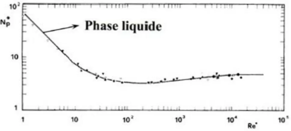
where Øv is the solid volume concentration. In this manner, they observed that the modified

power curve (Np* vs Re*) superimposes the single phase power curve (NP vs Re). Consequently,

the power consumption of solid-liquid mixing can be estimated if the single phase power curve is known, as well as the density of the suspension (defined as the total mass in the vessel divided by the total volume) and the volume fraction of particles (Figure 1-3).

Bujalski (Bujalski et al., 1999) determined the power number for the A-310 impeller (hydrofoil) for solid loading up to 40 wt% . They showed that by increasing the solid loading, the power number increases. At solid loading higher than 20 wt% the variation of power number showed different trends. At low impeller speeds (N<200 rpm) the power number is lower than that for the single phase. By increasing impeller speed the power number increases until it reaches a maximum value and then it slightly decreased. The constant value of the power number at higher impeller speeds was higher than that for the single phase and it is related to solid concentration, which affects the mixture density surrounding the impeller.

(36)

Figure 1-3: Power curve for solid suspension in compare with single phase (Pasquali et al., 1983)

Bujalski et al. related the lower power variation to bottom shape change by increasing impeller speed. They have mentioned that at low speed the presence of a solid layer at the bottom of the vessel redirected the flow and the overall effect is that the power number is reduced. By increasing impeller speed this layer starts to vanish and the power number increases.

Wu et al. investigated power number variation for PBT-D and RT at extreme solid concentrations (>50 vol %). They found, the power number of PBT increases at high solid concentrations while that of RT decreases (Wu et al., 2002). Increasing the power number for PBT can be explained in the same way as Bujalski et al. (Bujalski et al., 1999) did, but a reduction in the power number of RT was related to the fact that damping at high solid loading suppresses the dead flow zones at the back of the Rushton turbine blades leading to the reduction of drag. On the other hand there is no dead flow zone behind the Rushton turbine blades and increasing solid loading only increases skin friction and, accordingly, drag coefficient. Those results are in contrast with what has been reported by Angst and Karume (Angst and Kraume, 2006), who reported the reduction of the power number for the Pitched blade turbine.

(37)

1.3. Impeller for Solid-liquid Suspension

The impeller plays several tasks in the agitation vessel; to suspend solid particles and to disperse them effectively. Choosing the proper impeller to satisfy the required solid suspension with a minimum power requirement is the key for the technical and economic viability of the process. There are two regions at the tank bottom where recirculation loops are weak: underneath the impeller and at the junction of the tank base and wall. Njs is affected significantly by the region of

the vessel where the final portions of the settled solid particles are lifted into suspension. This region varies for different impeller types. Impellers are classified as radial or axial flow impellers. Flow pattern of axial and radial flow impellers are completely different. Differences in flow pattern leads to different solid suspension mechanisms. Radial flow impellers sweep particles toward the center of the vessel base and suspend them from an annulus around the center of the vessel bottom. On the other hand, axial flow impellers tend to suspend solid particles from the periphery of the vessel bottom. It is more difficult to lift particles from the center than drive them toward the corner. The flow pattern of axial flow impellers facilitates suspension in comparison to radial flow impellers.

Figure 1-4: Radial and axial flow pattern

For impeller selection it is important to identify which impeller can provide the required hydrodynamics for the process at lower power consumption. In addition it is necessary to have information on cloud height, solid concentration distribution, and mixing-reaction contributions to make the proper selection.

(38)

In a turbulent liquid, suspending solid particles can be considered as balancing energy supplied by a rotating impeller and energy needed to lift the solids. Axial flow impellers with high pumping efficiencies are most appropriate for solids suspension. These impellers generate a flow pattern which sweeps the bottom of tank and suspends the particles. Solid pickup from the vessel base is achieved by a combination of the drag and lift force of the moving fluid on the solid particle and the bursts of turbulent eddies originating from the bulk flow in the vessel (Paul et al., 2004).

In solid-liquid mixing with high viscosity continuous phases, usually two mechanisms are required: the first is used to reduce particle size distribution and the second to reach a uniform degree of dispersion homogeneity throughout the vessel. A combination of the impellers mentioned above can achieve this task, resulting in the integration of several mixing steps within one vessel. In practice, the following mixing systems are found in industry (Tanguy et al., 1997):

 Multiple intermeshing kneading paddles mounted on a carousel (planetary mixer).

 A main centered impeller associated with off-centered ancillary turbines located close to the vessel surface.

 Co-axial impellers of a similar type rotating at the same speed.

 Co-axial or contra-rotating coaxial impellers with different speeds.

The existence of a scientific basis behind the development of these types of mixing systems is rare, as they have been developed by empirical considerations and industrial experiences. Many studies were done to find more effective impellers for solid-liquid suspensions. These investigations have shown that axial impellers have better performances (Paul et al., 2004). Lightnin impellers, such as A100, A200, A310 and A320, are used in different studies. These impellers make high downward flow pumping. Using ligtnin impellers in a flow controlled operation, e.g. solid suspension, is more cost effective than other axial impellers (McDonough, 1992).

Cooke and Heggs reported that the hollow blade turbine is an efficient impeller for the solid-liquid mixing operations under gassed conditions (Cooke and Heggs, 2005). Bararpour investigated the dual shaft mixer consisting of a wall-scraping Paravisc and a high speed Deflo disperser (Bararpour et al., 2007). Lea employed a Standard 45˚ pitch 6-bladed turbine (Lea,

(39)

2009) and Sardeshpande et al. used a down-pumping, pitched 6-bladed turbine (PBTD-6) and a 4-bladed Hydrofoil (HF-4) in their work (Sardeshpande et al., 2009).

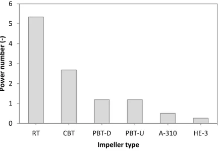
Lehn et al. compared power consumption for different impellers (Figure 1-5). Knowledge on power consumption in solid-liquid stirred tank is essential for proper design and operation (Lehn et al., 1999).

Figure 1-5: Ungassed power number of impellers in turbulent regime for different impellers (Lehn et al., 1999)

Some researchers have studied solid-liquid mixing in agitated vessels through experimental investigation (Baldi et al., 1978, Bujalski et al., 1999, Hicks et al., 1997, Wu et al., 2001) and some have employed CFD to explore the effect of impeller type on CH and Njs (Oshinowo, 2002,

Micale et al., 2004). Sardeshpande et al. investigated the effect of solid volume fraction and impeller speeds on the Njs, CH, power consumption, mixing time, and circulation time using

PBTD and HF impeller. They used tap water and glass bead particles (50-250 μm) with 1, 3, 5, and 7 vol% loading. They developed a new way of characterizing solid-liquid suspensions and liquid phase mixing using nonintrusive wall pressure fluctuation measurements. They found out that at higher solid loading (above 3 vol% ), cloud height measurements indicated different stages of suspension. By increasing impeller speed under certain conditions, cloud height is decreased. Interaction of incompletely suspended solids, a bed of unsuspended solids at the bottom and impeller pumping action cause such non-monotonic variations of cloud height with the impeller

0 1 2 3 4 5 6

RT CBT PBT-D PBT-U A-310 HE-3

Pow e r n u m b e r (-) Impeller type

(40)

speed (Sardeshpande et al., 2009). Giraud et al. showed that the optimal impeller speed has a significant effect on the degree of homogeneity. This speed should always be between two critical impeller speeds, Njs and the impeller speed for the maximum homogeneity, preferably

closer to the latter. Also, by increasing the particle size, the free settling velocity in solid suspension is increased and the extent of homogeneity is decreased (Guiraud et al., 1997).

Most of the studies on just suspended speed have been carried out in flat bottom vessels. A few work attempted to characterize Njs in dish bottom vessels (Buurman et al., 1986) or studied the

effect of tank bottom shape (Chudacek, 1985, Musil and Vlk, 1978). Ghionzoli et al. studied the effect of bottom roughness on Njs. They have reported that effect of bottom roughness is related

to particle size. For small particles size, suspension is helped by roughness. But by increasing dp

rough bottom begin to hinder suspension (Ghionzoli et al., 2007). The influence of the clearance on the flow pattern has been the subject of extensive studies. (Kresta and Wood, 1993, Bourne and Sharma, 1974b, Sharma and Shaikh, 2003). Montante et al. investigated transition in flow pattern for RT by decreasing impeller clearance by means of laser-Doppler anemometry (Micale et al., 2000, Montante et al., 1999). they also studied flow regime transition for RT by means of CFD tools For axial flow impellers (Montante et al., 2001, Micale et al., 2004, Micale et al., 2000). Sharma and Shaikh showed that all impellers with very low clearance (C/T <0.1) behave like the axial flow impeller and generate a single-eight loop flow. This low-clearance range is the most efficient condition for the impellers (Sharma and Shaikh, 2003). Foucault et al. utilized the determination theory of just-suspended speed that was developed by Zwietering, using Delfo, Sevin and Hybrid coaxial mixers. It was shown that for Newtonian or Non-Newtonian continuous phases, the capability of Sevin and Hybrid impellers to generate axial pumping was better than Deflo and they needed lower Njs (Foucault et al., 2004). Bararpour et al. studied the power

consumption and homogenization efficiency in a dual shaft mixer consisting of a wall-scraping Paravisc and Deflo disperser in the case of a highly viscous continuous phase. In their work, the power consumption by solid-liquid dispersion was detailed. They showed that Deflo provides good pumping capacity and increasing the rotational speed of the Deflo lowers the Paravisc power draw. They also explained the maximum and minimum power consumption by the possibility of the formation of particle agglomerates (Bararpour et al., 2007). Pinelli and Magelli studied the solid distribution in pseudo plastic fluid in a stirred tank with four Rushton turbines. They found out the concentration profiles of two different pseudo plastic liquids are qualitatively

(41)

similar with Newtonian liquid and the higher viscosity of the primary liquid makes the lower deviation from suspension homogeneity (Pinelli and Magelli, 2001). Fajner et al. studied the dispersion behavior of buoyant solid particles in multiple Rushton turbines. Due to the buoyant property, the solid concentration in this case is increasing from tank bottom to top, which is symmetrical to the profile of solid particles with higher density than continuous liquid. Moreover, the higher speed causes more uniform concentration distribution. They also pointed out that the solids loading has no effect on the concentration profile (Fajner et al., 2008). Kresta and Wood investigated the effect of the impeller clearance on the flow pattern generated by PBT in a fully baffled stirred tank. They concluded that by increasing the impeller clearance the angle of flow discharge from the axial direction toward the radial direction will be changed (Kresta and Wood, 1993). Hicks et al. studied solid suspension with four-bladed, 45° pitched blade turbines and Chemineer high-efficiency impellers. They reported that impeller type and physical properties do not strongly influence cloud height except for the fastest-settling solids (Hicks et al., 1997). Peker and Helvaci also reported that the degree of homogeneity decreases when the terminal velocity of the solid particles increases (Peker and Helvacı, 2007). A similar trend was also observed by Godfrey and Zhu (Godfrey and Zhu, 1994). Hoseini et al. investigated the effect of impeller type (LightninA100, A200, A310, and A320impellers), impeller speed, impeller off-bottom clearance, particle size (210–1500 mm), and solid concentration (5–30wt %) on the degree of homogeneity in an agitated tank. They developed CFD modeling to explore the effects of these parameters on mixing and compared their results with the experimental data. It was shown that the homogeneity of the system will be increased by increasing impeller power/speed. When homogeneity reaches the maximum, any further increase in impeller power/speed is not beneficial, but detrimental. The reason is the formation of regions with low solid concentrations inside the circulation loops at higher impeller speed. Hence, in a solid–liquid mixing system, the measurement of the optimal impeller speed as a function of the operating conditions and design parameters has a vital role in achieving maximum homogeneity (Hosseini et al., 2010a, Hosseini et al., 2010b). Tamburini et al. employed CFD modeling to investigate the dynamic behavior of the mixing of the silica suspension in a fully baffled mixing tank equipped with a radial flow impeller (Rushton turbine). They observed a high level of agreement between experimental results and relevant computational pictures (Tamburini et al., 2009). Ochieng et al. investigated nickel solids distribution with a four blade hydrofoil propeller in a stirred tank, using CFD and experimental

(42)

methods. They reported that for high solids loading, the turbulent dispersion force is very important. By increasing particle size and loading, axial concentration distribution decreases and the difference between axial solid concentrations at different elevations increases (Ochieng and Lewis, 2006a, Ochieng and Lewis, 2006b). Fradette et al. employed CFD modeling to explore the migration of particles in a stirred vessel and developed the diffusion model to predict the behavior of concentrated suspensions. The average behavior of a suspension in a three dimensional situation can be predicted with this model (Fradette et al., 2007a).

1.3.1. Maxblend Impeller

In the 1990’s, a wide impeller named Maxblend was designed by Sumitomo Heavy Industrials (SHI) Mechanical & Equipment. It combines two parts, a low paddle and a grid. The Maxblend is one of the most promising impellers of the new generation, due to its good mixing performance, its low power dissipation, its simple geometry that makes it easy to clean, and its capability of operating in a wide range of Reynolds numbers (Mishima, 1992, Kuratsu et al., 1995).

Figure 1-6: Schematic of the Maxblend impeller

The Maxblend impeller represents an interesting alternative to close-clearance impellers and it has been used in different processes. SHI uses the Maxblend for a variety of applications in liquid-liquid, liquid-solid and gas-liquid mixing. According to the manufacturer claims, the

(43)

Maxblend can handle processes from suspension polymerization and crystallization operation to high viscosity gas absorption. The Maxblend design idea originally comes from multi-stage impellers. As shown in Figure 1-7, the separation plan (interfering boundary) is formed by the upward and downward flow while the two multi-stage impellers are rotating. By combining the two impellers in a wide impeller, the boundary can be eliminated. Moreover, moving the impeller close to the bottom of the tank creates just one circulation flow in the tank. Finally, by adding the grid part, efficient mixing can be achieved. In addition, the simple shape of the impeller (no pitch, no angle, no spiral) makes the clean-up process easy and reduces the adhesion problem and the polymer blocks.

Multi-stage One-stage One circulation Efficient mixing boundary disappear

Figure 1-7: Concept of the Maxblend design (Iranshahi et al., 2007)

The top-to-bottom pumping induced by Maxblend is remarkable: the flow goes upward near the wall and downward in the center along the shaft. With regard to the flow pattern in the Maxblend mixer, it was proven that the paddle produces a strong tangential flow and a weak axial flow, generating a strong recirculation at the bottom of tank that causes flow segregation, while the grid part generates an axial pumping, with an upward motion at the vessel wall and a downward flow along the shaft. Therefore, four large loops are generated in the tank, two near the paddle (one in front and one behind) and two in the grid region (Figure 1-8). In fact, due to the symmetry, these four loops comprise two mixing structures: one at the bottom and one at the grid part (Iranshahi et al., 2007). The size of the two bottom circulation zones decreases by increasing the Reynolds number (Devals et al., 2008).

(44)

Figure 1-8: Effect of Reynolds numbers on flow pattern and velocity field for un baffled configuration: (a) Re = 80

(b) Re = 40 (Iranshahi et al., 2007)

There are different types of Maxblend, including: straight, wedge, modified N˚1, and modified N˚2, which are shown in Figures 1-9 and 1-10. The Maxblend modified N◦1 presents small apertures accounting for 1/3 of the paddle surface and the Maxblend modified N◦2 presents larger openings, about 2/3 of the bottom paddle surface. The shape of the Maxblend is known to influence the overall pumping capability. The wedge type is used for viscous applications while the straight-shaped Maxblend is preferred for the turbulent regime. The recirculation areas observed in high viscosity with the wedge Maxblend can be removed by making openings in the bottom paddle.

Figure 1-9: (a) Straight Maxblend impeller (b) Wedge Maxblend impeller