Dynamics, Control and Extremum Seeking of the Rectisol Process

UNIVERSIT´E DE MONTR´EAL

DYNAMICS, CONTROL AND EXTREMUM SEEKING OF THE RECTISOL PROCESS

MOHAMMAD GHODRATNAMA D´EPARTEMENT DE G´ENIE CHIMIQUE ´

ECOLE POLYTECHNIQUE DE MONTR´EAL

M´EMOIRE PR´ESENT´E EN VUE DE L’OBTENTION DU DIPL ˆOME DE MAˆITRISE `ES SCIENCES APPLIQU´EES

(G´ENIE CHIMIQUE) NOVEMBRE 2013

´

ECOLE POLYTECHNIQUE DE MONTR´EAL

Ce m´emoire intitul´e :

DYNAMICS, CONTROL AND EXTREMUM SEEKING OF THE RECTISOL PROCESS

pr´esent´e par : GHODRATNAMA Mohammad

en vue de l’obtention du diplˆome de : Maˆıtrise `es sciences appliqu´ees a ´et´e dˆument accept´e par le jury d’examen constitu´e de :

M. Srinivasan Bala, Ph.D., pr´esident

M. Perrier Michel, Ph.D., membre et directeur de recherche M. Abatzoglou Nicolas, Ph.D., membre

iii

To My parents, To whom I own everything I have. . .

ACKNOWLEDGEMENTS

Approaching the end of this period, I would like to thank those who helped realize the work done. First of all, It is with immense gratitude that I acknowledge the support of my supervisor, Professor Michel Perrier, for guiding me through out the path and for his patience and for showing me that it’s not hard to follow your passion. I would also like to thank the members of his team and my colleagues, Guillaume for helping me out whenever I needed his help and encouraging me. Didac, Samin , Masood, Javier and Prof. Srinivasan for sharing their knowledge with me. I feel also responsible to thank Prof. Zhu who reminded me that the right way starts from the basics.

I also appreciate the cooperation of the department’s informatics technician, Mehdi, and Prof. Francois Bertrand for allowing me to use the resources of URPEI to fulfill the requirements of this project.

I would also like to thank my former officemates at A-562, Ata, Majid, Ebrahim, Amirhosein, Richard,Patrice and Romain and my current officemates at URPEI, Julie, Bruno, Inci, Selim, Christopher, Benoit, Ebrahim and David for creating a friendly and warm environment. I wish also to show my profound gratitude to my parents, my brother and sister, who where on my side and supported me during this time, and to as well for their encouragement and help.

I also wish to thank my friends at AECSP, who made my experience at Polytechnique fun, my friends and family in Iran all my friends in montreal,Shahab, Shervin, Helia, Milad, Amin, Amir, Danial,Tareq, Fanny and their son Tristan.

Since there’s the rest of the page left, I would like to thank Metallica, Linkin park, Breaking Benjamin, Three days grace, 30 seconds to mars and Hoobastank for making great music that helped me significantly while running simulations.

v R´ESUM´E

Pendant la derni`ere d´ecennie, les bioraffineries bas´ees sur la gaz´eification ont fait l’objet de nombreuses ´etudes dans le cadre des e↵orts mondiaux visant `a remplacer les combustibles fossiles qui produisent de l’´energie et des produits chimiques `a valeur ajout´ee. Une partie importante de ces bioraffineries est l’unit´e de purification des gaz de synth`ese issus de l’oxy-dation partielle, qui enl`eve le CO<sub>2</sub> et l’H<sub>2</sub>S. Un des proc´ed´es de purification consid´er´e dans ces ´etudes est le Rectisol. Ce proc´ed´e est utilis´e car il est plus environnemental et requi`ert moins de coˆuts d’investissement et d’op´eration par rapport `a d’autres proc´ed´es similaires. Afin de faire l’´etude dynamique de ce proc´ed´e, une simulation en r´egime permanent a, d’abord, ´et´e men´ee `a l’aide du logiciel Aspen plus R. Le comportement de ce mod`ele a ´et´e ´etudi´e et

valid´e par rapport aux donn´ees trouv´ees dans la litt´erature. Des vannes de contrˆole ont ´et´e plac´ees dans les endroits n´ecessaires. Apr`es avoir dimensionn´e les ´equipements, tels que les s´eparateurs, les vannes, les puisards de colonne et les condenseurs, les pressions ont ´et´e v´eri-fi´ees pour que celles des courants entrants `a l’´equipement s’accordent avec la pression dans la zone d’entr´ee de l’´equipement. Le mod`ele a ´et´e export´e en Aspen plus Dynamics et les e↵ets des entr´ees de mod`ele et des perturbations ont ´et´e ´etudi´es sur les variables de sorties. Vu que la composition et les caract´eristiques de la biomasse gaz´eifi´ee varient, la composition et la quantit´e d’impuret´es du gaz produit changent aussi. Ceci cr´ee alors des variations au niveau de la puret´e du gaz de synth`ese et des sous-produits de l’unit´e de purification du gaz. Dans une usine, il est important de garder les compositions de produits aussi constantes que possible afin de ne pas cr´eer de perturbations dans les unit´es en aval. Pour surmonter ces va-riations, un sch´ema de recherche d’extremum adaptatif a ´et´e implant´e. Il consiste `a optimiser une fonction objectif quadratique des compositions de produit pour laquelle la relation entre les variables ind´ependantes et la fonction objectif est inconnue.

Pour que la recherche d’extremum soit bien efficace, une structure de contrˆole r´egulateur sensible, `a l’´echelle de l’usine, est n´ecessaire. Les proc´ed´es de purification des gaz bas´es sur l’absorption ont tous un courant de recyclage du solvant, ce qui peut ˆetre probl´ematique au niveau du contrˆole des proc´ed´es. Une recherche a donc ´et´e men´ee sur les techniques de contrˆole conventionnelles et avanc´ees. Quatre strat´egies potentielles de contrˆole ont ´et´e mises en œuvre et leurs performances ont ´et´e analys´ees. Ces quatre strat´egies sont : PI, MPC cen-tralis´e, MPC distribu´e et MPC d´ecentralis´e. La raison pour laquelle nous avons choisi des contrˆoleurs MPC est qu’ils peuvent envisager syst´ematiquement, `a la fois, les interactions entre les variables et les contraintes sur les entr´ees et sorties dans les calculs de contrˆole.

Parmi les quatre strat´egies, MPC distribu´e et MPC centralis´e sont apparue comme les plus performante en terme de rejet de perturbations du flux d’entr´ee et de suivi des consignes. Pour ces deux strat´egies, un sch´ema de recherche d’extremum adaptatif `a plusier entre´es a ´et´e con¸cu et appliqu´e et leurs performances ont ´et´e ´etudi´ees pour di↵´erentes fr´equences de signal d’excitation. Les r´esultats ont montr´e que, pour la fr´equence la plus performante, les deux combinaisons de structures d’optimisation et de contrˆole ont un comportement identique. Pour finir, la combinaison de la recherche d’extremum adaptatif avec MPC distribu´e a ´et´e choisie comme structure d’optimisation et de contrˆole pour l’usine de Rectisol ´etudi´ee. En e↵et, MPC distribu´e est moins sensible aux pannes et le contrˆole de l’installation ne d´epend pas d’un seul agent de contrˆole. En conclusion, nous avons rendu le proc´ed´e Rectisol plus robuste aux perturbations sur la composition et le d´ebit d’entr´ee afin que l’usine soit capable de garder ses compositions de produits les plus proches possibles des sp´ecifications souhait´ees.

vii ABSTRACT

Gasification based biorefineries have been studied in the past decade as part of a global e↵ort to replace fossil fuels to produce energy and added value chemicals. An important part of these biorefineries is the acid gas removal units, that remove CO₂ and H₂S from the produced synthesis gas. One of the acid gas removal processes associated in these studies is Rectisol. Rectisol has been chosen since it’s environmental friendly and requires a lower amount of operational and capital costs compared to its opponents.

To carry out a dynamic study of the process, as a first step, a steady-state simulation was carried out in Aspen Plus R. The steady-state behavior of the columns were studied and

validated based on data found in the literature. Control valves were placed in all the necessary places. After sizing the equipment, such as seperation drums, valves and column sumps, the pressures were varified, so that the pressure at the inlet of each equipment corresponds to incoming stream. Later on the model was exported to Aspen plus dynamics and the e↵ect of di↵erent inputs and disturbances on the outputs were studied.

Due to the fact that the composition of the gasified biomass varies, the composition and the amount of impurities in the gasification gas also varies This creates variations in the purities of the syngas and byproducts of acid gas removal units. In any chemical plant it is important to keep compositions of products as constant as possible so that we don’t create perturbations in downstream units. To overcome these variations an adaptive extremum control scheme was implemented that optimizes a quadratic objective function of product compositions, while the relation between the objective function and its independent variables is unknown. For the adaptive extremum seeking control to be e↵ective, a responsive plantwide regulatory control structure is required. Absorption based gas cleaning processes like Rectisol all have a recycle flow of solvent. This recycle flow can always be problematic from a process control point of view. Thus a search was conducted amongst the conventional and advanced control techniques. Four potential control strategies were implemented and their performance was analyzed. These four strategies were Multiloop PI, Centralized Model Predictive Control (MPC), Decentralized MPC and Distributed MPC. The reason we have chosen MPC is that these controllers can systematically consider process variable interactions and input and output constraints in their control calculations. Among the four, distributed and centralized MPC were found to be most e↵ective in terms of rejecting input flow disturbances and tracking setpoints. Keeping this fact in mind a multivariable extremum-seeking scheme was designed and implemented on these two types of controllers and their performance was studied for

di↵erent dither signal frequencies. The results showed that at the proper frequency, both combination of optimization and control structures have identical behavior.

At the end the combination of adaptive extremum seeking and Distributed MPC was chosen as the optimizing and control structure for the studied Rectisol plant, since Distributed MPC is more fault tolerant and the control of the plant will not depend on a single control agent. In conclusion, Rectisol has been robustified to the composition and flowrate of the input and the plant is able to keep its product compositions as close as possible to the desired specifications.

ix TABLE OF CONTENTS DEDICATION . . . iii ACKNOWLEDGEMENTS . . . iv R´ESUM´E . . . v ABSTRACT . . . vii TABLE OF CONTENTS . . . ix LIST OF TABLES . . . x LIST OF FIGURES . . . xi

LIST OF APPENDIXES . . . xii

LIST OF SYMBOLS AND ABREVIATIONS . . . xiii

CHAPTER 1 INTRODUCTION . . . 1 1.1 Motivation . . . 1 1.1.1 Process configuration . . . 1 1.1.2 Absorption mechanisms . . . 2 1.2 Problem definition . . . 5 1.3 Objectives . . . 6 1.4 Thesis orginization . . . 6

CHAPTER 2 LITERATURE REVIEW . . . 7

2.2 Plantwide control of processes with recycle . . . 9

2.3 Linear Model Predictive Control . . . 10

2.4 Distributed Linear Model Predictive control . . . 12

2.5 Adaptive extremum seeking control and Realtime optimization . . . 13

CHAPTER 3 Methodology . . . 15

3.1 Development of a dynamic model . . . 15

3.1.1 Development of the steady state model . . . 15

3.1.2 Forming the dynamic platform . . . 24

3.2 Identification of a linear model for MPC . . . 30

3.2.1 Identification of dynamic models . . . 30

3.2.2 Validation of the dynamic model . . . 37

3.3 Centralized linear MPC design . . . 37

3.4 Distributed MPC Design . . . 43

3.5 Design of the adaptive extremum seeking loop . . . 46

CHAPTER 4 RESULTS AND DISCUSSION . . . 50

4.1 Tuning of di↵erent control schemes . . . 50

4.1.1 Multiloop PI tuning . . . 50

4.1.2 Centralized MPC tuning . . . 51

4.1.3 Distributed and Decentralized MPC tuning . . . 52

4.2 Comparison of controller performance . . . 53

4.3 Adaptive extremum seeking . . . 57

4.4 Summary of results . . . 64

CHAPTER 5 CONCLUSIONS AND RECOMMENDATIONS . . . 65

5.1 Conclusions . . . 65

xi

REFERENCES . . . 67

LIST OF TABLES

Table 2.1 Industrial linear MPC products (Qin and Badgwell, 2003) . . . 11

Table 3.1 Feed Composition . . . 19

Table 3.2 Vessel dimensions . . . 23

Table 3.3 Pressure drop per tray . . . 24

Table 3.4 List of PID controllers . . . 26

Table 3.5 Inputs and Outputs of model . . . 31

Table 3.6 Inputs and Outputs of model . . . 33

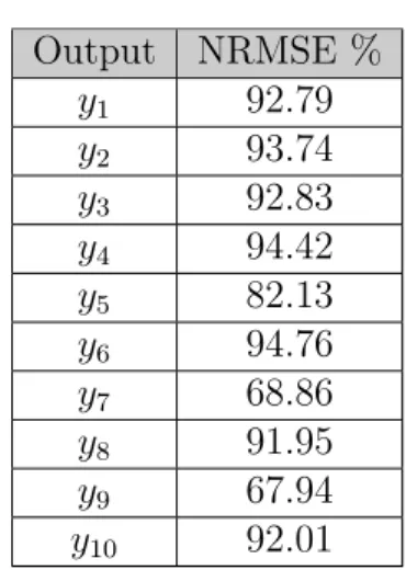
Table 3.7 Goodness of fit of model . . . 34

Table 3.8 Validation of model . . . 37

Table 3.9 Inputs and Outputs of model . . . 44

Table 4.1 Tuning of PI controllers . . . 51

Table 4.2 Results for Disturbance rejection . . . 53

Table 4.3 Results for Set point tracking . . . 54

Table 4.4 Comparison of loss of precision for setpoint tracking . . . 54

xiii

LIST OF FIGURES

Figure 1.1 Rectisol configuration used . . . 4

Figure 2.1 Standard Rectisol configuration (Hiller et al. (2000),p.96) . . . 7

Figure 2.2 Selective Rectisol configuration (Ranke, 1977) . . . 8

Figure 2.3 Evolution of industrial MPC technology (Qin and Badgwell, 2003) . . 12

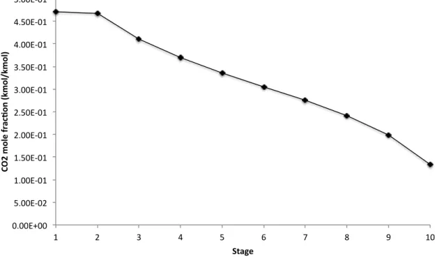
Figure 3.1 Process flow diagram of total CO₂ and H₂S removal Rectisol (Larson et al. (2006),p.43) . . . 16

Figure 3.2 Process flow diagram of the Rectisol used . . . 18

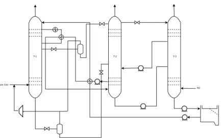
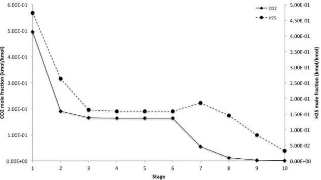
Figure 3.3 CO₂ and H₂S mole fraction profiles (gas phase) in the absorber . . . . 21

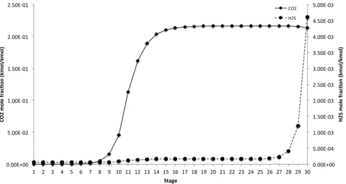
Figure 3.4 CO₂ mole fraction profile (gas phase) in the H₂S concentrator . . . 21

Figure 3.5 CO₂ mole fraction profile (gas phase) in the CO₂ stripper . . . 22

Figure 3.6 CO₂ and H₂S mole fraction profiles (gas phase) in the solvent regenerator 23 Figure 3.7 Process flow diagram of the rectisol with PID controllers . . . 28

Figure 3.8 Schematic of the Aspen dynamics flowsheet . . . 29

Figure 3.9 Identification signals . . . 32

Figure 3.10 Model output vs identification data . . . 35

Figure 3.11 Step response of the identified model . . . 36

Figure 3.12 Simulink layout of Centralized MPC . . . 42

Figure 3.13 Simulink layout of centralized MPC, plant subsystem . . . 42

Figure 3.14 Simulink layout of centralized MPC, controller subsystem . . . 43

Figure 3.15 Information flow suggested by Rawlings and Stewart (2008) . . . 45

Figure 3.16 Information flow of our DMPC . . . 45

Figure 3.17 Adaptive extremum seeking principle . . . 47

Figure 3.19 Settling time for the closed loop system for a) 2nd_{, b) 5}th_{, c) 10}th_output

of the system with Centralized MPC . . . 48 Figure 3.20 Combination of adaptive extremum seeking with a) Centralized MPC

and b) Distributed MPC . . . 49 Figure 4.1 Performance of controllers for disturbance rejection . . . 55 Figure 4.2 Performance of controllers for setpoint tracking . . . 56 Figure 4.3 Performance of adaptive extremum seeking with centralized MPC . . . 59 Figure 4.4 Performance of adaptive extremum seeking with Distributed MPC . . . 61 Figure 4.5 Tracking performance of distributed MPC for setpoints generated by

adaptive extremum seeking . . . 62 Figure 4.6 Setpoint trajectories for a) CMPC at 0.01 Hz, b) DMPC at 0.01 Hz,

c) CMPC at 0.02 Hz, d) DMPC at 0.02 Hz, e) CMPC at 0.1 Hz and f) DMPC at 0.1 Hz . . . 63

xv

LIST OF APPENDIXES

LIST OF SYMBOLS AND ABREVIATIONS

List of Abbreviations

ARX Auto Regressive with external input COD Constant Output Disturbance DMC Dynamic matrix control DPS Distributed Parameter system FC Flow Controller

FIR Finite Impulse Response FSR Finite Step Response

GPC Generalized Predictive control

IGCC Integrated Gasificatiom combined Cycle IMC Internal Model Control

ISE Integral of Squared Error LC Level Controller

LQG Linear Quadratic Gaussian LSS Linear State Space

MIMO Multi Input- Multi Output MISO Multi Input- Single Output MPC Model Predictive Control

NRMSE Normalized root mean square error PC Pressure Controller

QDMC Quadratic Dynamic Matrix control RTO RealTime Optimization

SVD Singular Value Decomposition TC Temperature Controller TF Transfer function

List of Symbols

A, B, C space state model parameters a, b constraint matrices

d measured disturbance

F state matrix in prediction generation

xvii

G disturbance matrix in space state model Gp approximation of system model

H QP matrix J MPC or LQG obejctive function k discrete time kc proportional gain of PI Np Prediction Horizon Nc Control Horizon P Pressure

Q state or output weighting matrix R input weighting matrix

ui ith Input of system

x states of augmented system xmi ith state of system

yi ith Output of system

ˆ

yi output of the identified model

Y vector of predicted outputs U predicted input sequence

¯

U input sequence of other subsystems

disturbance matrix in prediction generation IMC tuning parameter

⌧I Integral time of PID

⌧P time constant of approximated model

✓ dead time of approximated model

input of other subsystems matrix in prediction generation input matrix in prediction generation

CHAPTER 1

INTRODUCTION

Work done in this thesis can be divided in two general sections, first the process enginee-ring section which focuses on the design, steady-state and dynamic simulation of a Rectisol plant and second the control and real time optimization section. In this chapter we will brie-fly provide a background on these two subjects and describe the motivation and objectives behind our work. The structure of the thesis is also provided at the end of this chapter.

1.1 Motivation

Removal of acid gases, mainly CO₂ and sulphuric compounds such as H₂S and COS, is used for the purification of a tailgas, intermediate or final product gas stream. The purpose of this purification can be environmental and safety issues , operating constraints, or both. Acid gas removal processes are utilized in many industries such as the oil and gas, power plants and most recently in the gasification based biorefineries.

There are many reasons for removal of sour components in a gas, one is environmental regulations. For example in many regions there are regulations on the amount of carbon and sulfur in gas emissions of a power plant or chemical unit. Another reason can be the quality of a final product, for example if a plant is producing syn gas for combustion, the CO₂ is removed to increase the heating value of the gas and sulfur compounds have to be removed due to safety issues. Also another constraint is the requirement of downstream processes, for example the syn gas being sent to a Fischer Tropsch unit should not contain sulfur compounds to prevent their reaction with the catalyst and to protect the catalyst.

These processes consist of two main sections : – The absorption section.

– The regeneration section.

1.1.1 Process configuration

The absorption section consists of one or two absorption columns where the gas is contac-ted with the lean solvent and impurities are absorbed. The regeneration section contains

strip-2

pers and distillation columns where the rich solvent is stripped from the absorbed impurities. The configuration of the absorption and regeneration sections depends on the pressure, tem-perature and composition of the contaminated gas, the upstream and downstream processes and the use of the syngas, such as production of ammonia, methanol, or even combustion gas.

1.1.2 Absorption mechanisms

Depending on the absorption mechanism used for separation acid gas removal processes are divided into two groups :

– Chemical absorption. – Physical absorption.

In chemical absorption the contaminants form a chemical bond with the solvent, while in phy-sical absorption the contaminats are absorbed only based on their solubility in the solvent and no significant chemical reaction occurs. Examples of chemical absorption processes are Monoethanolamine (MEA), Diethanolamine (DEA), Methyl diethanolamine (MDEA), Die-thyleneglycol (DEG) and TrieDie-thyleneglycol (TEG). As we see these solvent are all of a basic nature and thus react with the acid gas components to absorb it. Examples of physical ab-sorption processes used for acid gas removal are Rectisol which uses methanol as solvent, Purisol with N-methyl-2-pyrrolidone (NMP) as solvent, Selexol with a mixture of dimethyle-ther and polyethylene glycol. A third group of processes use a mixture of both physical and chemical solvents. Examples of these processes are Amisol and the Selefining process.

The process studied in this work is a physical absorption process named Rectisol. Compared to many similar processes, Rectisol is an economical and environmental friendly candidate for purification of gases produced by partial oxidation of carbon containing material. It is widely considered as part of many gasification based biorefinary schemes due to its design and operation flexibility, capability in removal of sulphuric compounds and CO₂ in ppm ranges, and its potential for energy integration. The advantages of Rectisol is that in this process the solvent does not foam in contact with the sour gas, the solvent is not corrosive and it can be easily regenerated by flashing at low pressures. But it also comes with a disadvantage which is the relatively high refrigeration energy requirement which leads to higher operating costs (Olajire, 2010).

Based on the area of application, Rectisol can have many configurations. If the absorption section consists only of one column, or in other words if the absorption of CO₂ and H₂S is done at the same time, the process is said to be single stage. But if the absorption of H₂S and CO₂ is done in two separate columns, the process is said to be two stage. Also if CO₂ and

H₂S are disposed of in the same stream the process is non-selective, and if CO₂ and sulfur compounds are disposed of in separate streams, the process is called selective (Ranke and Mohr, 1985).

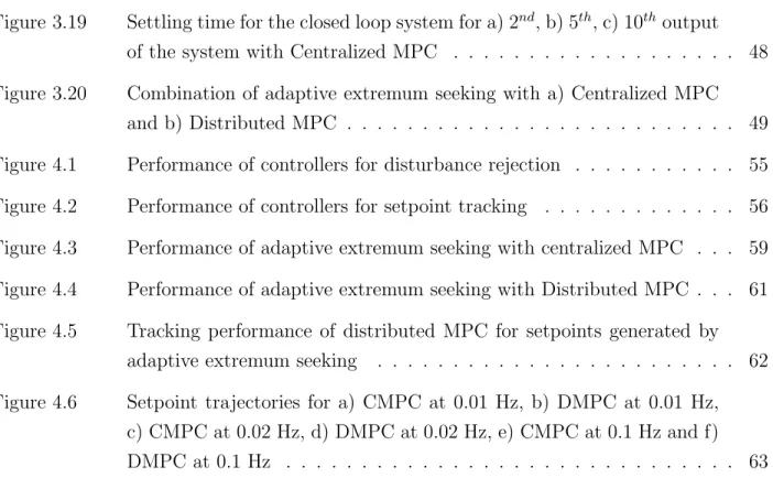
The configuration we used in this work is two stage and selective. Figure 1.1 shows this configuration :

4 F ig ur e 1.1 R ec tis ol co nfig ur at io n us ed

As we can see the syngas enters the bottom absorber ( which actually consists of two columns on top of each other) where it is contacted with partially loaded solvent, mostly containing CO₂, to absorb the H₂S, and also CO₂ . The remaining amount of CO₂ is ab-sorbed in the top section of the column in contact with the lean solvent. The solvent is withdrawn from the absorber at the end of each section, and flashed to remove the valuable components like H₂, CO and CH₄. While part of the liquids from the first section is sent to the third column, the remainder is sent to the second column. In the second column which is also called the ”H₂S Concentrator” the rich solvent is heated up to a temperature where mainly CO₂ is stripped from the liquid. The gas product of the H₂S concentrator is 98 vol% CO₂. The pressure of the liquid product is dropped and it is flashed, the resulting gas stream is recycled back to column as stripping gas and the liquid phase is sent to the third column. The third column which is called the ”CO₂stripper” removes the remaining CO₂ from the rich solvent using a stream of pure nitrogen.The gas product of this column is approximately half CO₂ and half N₂. The liquid product is divided into two streams, while the smaller portion is recycled to the H₂S concentrator, the larger portion is sent the solvent regenerator. The solvent regenerator is a conventional distillation column, where the remaining sour compo-nents are removed from the solvent using distillation and the lean solvent is cooled and sent back to the absorber.

1.2 Problem definition

The problem assumed to be associated with the Rectisol process studied in this thesis is that the feed composition and flowrate to the Rectisol process may vary depending on the operating conditions of the gasifier, the biomass composition and many other parameters. In order for the process to react to these variations and keep the products as close as possible to the specified standards, adaptive extremum seeking control was used.

As seen in the previous section, the process is complex in terms of recycle streams. Such a process is multivariable and highly interactive and like many other chemical processes shows nonlinear behaviour. For the adaptive extremum seeking control to be functional and to reject measurable and unmeasurable disturbances and also for the process to adapt to new operating conditions a fast interactive regulatory control structure is required.

In this context a search for an implementable multivariable control structure was done and an adaptive extremum seeking scheme was designed that keeps the product specifications as close as possible to their standards.

6

1.3 Objectives

The general objective associated with this work is : to implement adaptive extre-mum seeking control on the Rectisol process to optimize its performance in the presence of perturbations. In this context the following specific objectives were declared to achieve our General objective :

– To develop a dynamic model for Rectisol

– To design and implement a plantwide regulatory control structure on the dynamic model

The hypothesis linked to our objectives is that adaptive extremum seeking can help improve the performance of the process especially in the presence of unmeasurable disturbances.

1.4 Thesis orginization

This thesis commences with a brief literature review (Chapter 2) on the Rectisol process and its simulation, a plantwide control solution to recycle processes, Linear MPC, Distributed Linear MPC and at the end adaptive extremum seeking control.

In Chapter 3 the methodological concepts used, will be described. The latter includes the development of a dynamic model in Aspen plusRDynamics, design of a centralized and

distributed MPC structure and design of a multi input adaptive extremum seeking scheme. In chapter 4 the results of the regulatory control structure will be presented independently and compared using existing criteria and interpreted.Then the adaptive extremum seeking control layer will be implemented on some of these structures and their performance will be compared in terms of control and optimization.

In the final chapter (chapter 5) a conclusion will be made from the results presented in the previous chapter and the best regulation and optimization structure will be chosen.

CHAPTER 2

LITERATURE REVIEW

In this chapter we briefly review the literature on Rectisol, linear model predictive control, distributed MPC and adaptive extremum seeking.

2.1 Rectisol

Rectisol is known to be an economical process for acid gas removal of partial oxidation products(Weiss, 1988). As found in Ullmann’s Encyclopedia of industrial chemistry, it has been cited by Ranke that the Rectisol process was at first invented by Lurgi in 1950 and later on further developed, in cooperation with Linde (Hiller et al., 2000). In general it is used for the purification of partial oxidization gases, and has di↵erent configurations based on the purpose of its application. Ranke and Mohr (1985) classify di↵erent configurations of the process into two main classes, non-selective and selective. The selective systems have at least two sour gas products, one sulfur free CO₂ stream, and a sulfur stream which is fed to a Clause unit. The non-selective systems only have one sour gas stream containing both CO₂ and sulfur compounds. The standard Rectisol configuration is of the non selective type. Its flow diagram can be seen in figure 2.3. Ranke (1977) modified this flow diagram to create a_{96 Gas Production}

Figure 45. Standard Rectisol process for simultaneous removal of H2S and CO2

a) Absorber; b) Flash tower; c) Hot regeneration; d) Condenser; e) Methanol – water column in this desorption step and not by the

refrigera-tion unit. This phenomenon is often referred to as the “autorefrigeration effect”. In the fine wash

sectionof the absorber, only the residual acid gases are removed. Therefore, little heat of ab-sorption is released in the fine wash section and the temperatures remain low. Moreover, there is a smaller quantity of gas to be treated in the fine wash section. Therefore, solvent demand in the fine wash section is considerably lower than that in the main section of the absorber. This is de-sirable in view of the high investment and utility costs for hot regeneration.

In Fischer – Tropsch synthesis, SNG, and town gas plants, carbon dioxide must only be re-moved to a final content of 1 – 2 %. This value can even be reached in the main wash part with flash-regenerated methanol. The fine wash part then has to be designed only for removal of hy-drogen sulfide and carbonyl sulfide, which re-sults in a lower solvent rate, normally one-tenth of the total amount of solvent withdrawn from the bottom, due to the higher solubility of these components.

Downstream of hot regeneration, a metha-nol – water distillation column is used to sepa-rate water entering with the raw gas. To prevent icing in the cooling section of the raw gas, a small amount of methanol is injected upstream of the heat exchanger. The mixture of methanol and water is withdrawn and fed directly to the distillation column. A refrigeration unit is used to cover cold losses in the plant due to surge

energy, incomplete heat exchange, unrecovered heat of absorption, and insulation losses. An am-monia absorption refrigeration unit can be ad-vantageously applied if low temperature (130 – 200 C) waste heat is available.

The standard Rectisol process combines all absorbed gases in a single acid gas stream. The sulfur compounds are thus diluted with the entire absorbed volume of carbon dioxide. (Referred to the raw gas specification in Table 24, only 0.9 vol % of hydrogen sulfide [example 2] and only 1.8 vol %, of hydrogen sulfide [example 4] in the off-gas are typical of the standard process with complete removal of carbon dioxide.) The off-gas with this low sulfur content is not suitable for sulfur recovery in a Claus process. Other sul-fur recovery processes must be applied such as liquid-phase oxidation (see 5.4.3) or adsorption. The standard Rectisol process is therefore ad-vantageously applied for gases from low-sulfur feedstock.

Selective Rectisol Process. Initially the

se-lective Rectisol process was introduced to pro-duce an off-gas rich in hydrogen sulfide which could be processed in a Claus plant for sulfur recovery. Pure carbon dioxide is produced as a second product with a total sulfur content in the low ppm range. This stream can be vented to at-mosphere or utilized, for example in urea plants, which are often built in conjunction with ammo-nia plants, or recovered in food grade (see Sec-tion 6.3),or can be used for enhanced oil

recov-Figure 2.1 Standard Rectisol configuration (Hiller et al. (2000),p.96)

8

2.2 shows the proposed configuration.

Figure 2.2 Selective Rectisol configuration (Ranke, 1977)

Ranke and Mohr (1985) have also compared the selective and non-selective configurations considering energy consumption and performance in di↵erent applications. They have also listed a few applications such as ammonia production and methanol production. They also studied the integration of di↵erent processes with Rectisol such as shift gas conversion, sulfur production and cryogenic separation.

The number of absorption columns can also be di↵erent, single stage Rectisol consists of only one wash column while two-stage Rectisol consists of two. Two-stage Rectisol is mostly used along with the shift conversion process in ammonia and methanol plants where the shift conversion is done between the two stages of the wash (Weiss, 1988).

Literature on simulation of Rectisol itself is very limited, and it has been mainly studied as part of another process and mainly in steady state. Preston (1981) has developed a steady state model of Rectisol using the AspenR software. A non-selective configuration has been

modeled. The Redlich-Kwong-Soave equation-of-state was found suitable and the coefficients were found using experimental data. The model was developed to obtain mass and energy balances and to predict the composition of clean product gas by varying di↵erent paramaters and operating conditions. The overall regenerated solvent recycle loop was not closed to obtain convergence.

As part of a Dynamic model for IGCC, only the absorption section of Rectisol was modelled using the Dymola software. Equilibrium stages where considered and it was assumed that the system obeys the ideal gas - Henry law. The steady state results of this simulation where validated by results from Aspen Plus and Chemcad (Heil et al., 2009).

Many works has been done on dynamic modelling and simulation of other acid gas removal processes that are similar to Rectisol from a systems engineering point of view. The models are either created by combining first principle models of individual units or by using commercial software like AspenRPlus Dynamics (Lin et al., 2010; Harun et al., 2012).

2.2 Plantwide control of processes with recycle

Design of a plantwide control procedure for cascaded unit operations without any recycle streams was developed over half a century ago and has been widely used in the industry ever since (Buckley, 1964). But when a process contains recycle streams these techniques might cause instabilities through what is called ”the snowball e↵ect”. The dynamic behaviour of these systems have been studied and analyzed in detail by Luyben. In his work Luyben has used a Reactor/Separator example with a linear model (Luyben, 1993).

Later on Luyben (1994) proposes that in order to deal with the mass recycle loop , at least one of the flows in the in liquid recycle loop has to be flow controlled. The same concept can be applied on energy recycle loops. Once this is done conventional plantwide control procedures can be used. Tyreus and Luyben (1993) have also studied the snowball e↵ect in a one reactor, two separators configuration with two recycle streams, where a second order reaction takes place in the reactor, and have once again reached the conclusion that the flow-rate should be fixed at-least in one stream of the recycle loop. It has been shown that fixing the flow rate in the recycle loop at the fresh feed inlet can be advantageous compared to other alternatives (Bildea and Dimian, 2003).

By analyzing Luyben’s structure we can see that it takes away the possibility of optimizing the plant’s production rate. We can also see that snowball e↵ect can be dealt with by redoing the process design, in this case by increasing the reactor volume so that the larger volume of the reactor can damp the oscillation of the recycle loop . Larsson et al. (2003) pointed out that by defining an objective function and a set of active constraints we can develop a self optimizing control structure to regulate and optimize the plant’s performance. They later on point out that a MPC controller can explicitly handle the constraints. Seki and Naka (2008) have used Larsson’s self optimizing control structure as their regulatory layer and implemented a MPC as the supervisory layer to optimize the process economy.

The Tennessee Eastman process is another example of processes with a recycle stream. This process is nonlinear and open loop unstable. Amongst the first attempts to stabilize this process was the work of McAvoy and Ye (1994). They developed a multi loop PID structure using steady-state analysis, relative gain analysis, Niederlinski index and disturbance analysis. Ricker and Lee (1995) mention that Palavajjhala et al used PI controllers alongside with

10

Dynamic matrix control (DMC) to control this problem. The PI controllers give a partially open loop stable plant. Ricker formed a nonlinear model of the partially open loop stable plant and formed an MPC controller that linearizes the model at each time step. The Tennessee Eastman process is a benchmark for many control topics and a vast amount of literature can be found on this subject.

2.3 Linear Model Predictive Control

Roots of MPC can be traced back to Linear Quadratic Gaussian (LQG). In LQG for a linear time invariant discrete system in the form of :

x(k + 1) = Ax(k) + Bu(k) + Gw(k)

y(k) = Cx(k) + ⇠(k) (2.1)

where w(k) and ⇠(k) are the state disturbance and measurement noise, considered to be zero mean independent Gaussian noise, an objective function in the following form is formulated :

J =

1

X

i=1

xT_i Qxi+ uTi Rui (2.2)

Q and R are tuneable weighting matrices. By replacing u = Kx(k) in equation 2.2 the objective function is minimised for K which is the gain. The optimization is done o✏ine once, and the gain is implemented in the control loop. MPC is an extension of LQG in the sense that it controls the plant by optimizing a similar objective function, but the optimization is done at each time step for the current states of the system and it has a finite horizon (Qin and Badgwell, 2003).

In General MPC needs an internal model to generate the vector of predictions that represent the future dynamic behaviour of the plant. This model can be in the state space form, polynomial, or can even be a matrix of transfer functions. MPC also has an optimizer that tries to bring the vector of predictions generated by the internal model close to the reference trajectory by solving an optimization problem. This optimization problem can be constrained or unconstrained.

min

U(Y Yref)

T_{Q(Y Y}

ref) + UTR U (2.3)

The first works on MPC were carried out by Cutler and Ramaker (1980). They used linear step response models and formed an unconstrained multivariable control algorithm which is called Dynamic Matrix Control. This algorithm is advantageous compared to a multiloop

PID structure since it considers the interactions between variables but it does not explicitly handle constraints. DMC is considered as first generation MPC. Garcia and Morshedi (1986) reformulated the DMC problem into a Quadratic programming problem that can find the plant’s input by considering the constraints as part of the solution. This technique is cal-led Quadratic Dynamic Matrix control (QDMC). QDMC is considered as second generation MPC.

Clarke et al. (1987) have used input-output models to find the predictions. They showed that as long as the input-output correlation is rich enough, the predictive controller formed by this model is able to control the system even in the presence of non-minimum phase behaviour, open loop instability or unknown dead-time. This technique is called Generalized Predictive Control. As promising as it seems, this technique cannot handle multivariable constrained systems well (Morari and Lee, 1999).

MPC has been formulated in the state space format (Morari, 1990). In this manner, many useful theories can be applied to it and it also facilitates the extension of MPC to more com-plex cases. State space MPC needs the value of the states to carry out the calculations. These values can either be measured from the plant (if possible) or be provided by a state estimator. Wang and Young (2006) have proposed a method where non-minimal state space models are formed using input output data or even using transfer functions. They also augmented the model with integrators to enable o↵set free tracking. Previously to handle modelling error and o↵set, at each sampling interval the error between the process output and the model prediction at that instant was calculated and was fedback to the controller as a constant dis-turbance over the prediction horizon (Constant Output Disdis-turbance (COD)). Another idea is using a Kalman filter.

In the third generation MPC, new features are mainly use of state space models, an explicit description of disturbance models, the integration of a Kalman filter for state estimation and unmeasured disturbances and the introduction of soft and hard constraints to insure the fea-sibility of a solution by MPC. Examples of this generation are Shell multivariable optimizing control (SMOC), IDCOM-M by Setpoint Inc. and HIECON by Adersa . In terms of industrial application, MPC is pretty mature and has been applied in the industry for years. Aspen Technology Inc. and Honeywell are the two leaders in industrial MPC development. They have developed the fourth generation of MPC controllers which consider model uncertainty and enable multiple optimization levels (Qin and Badgwell, 2003). Table 2.1 shows a list of industrial linear MPC products.

12

Table 2.1 Industrial linear MPC products (Qin and Badgwell, 2003) Company Aspen Tech Honeywell Adersa Invensys SGS

Product DMC-plus RMPCT PFC Connois SMOC

Model Type FSR ARX,TF LSS,TF,ARX ARX,FIR LSS

Feedback COD COD COD COD KF

In recent years the MPC landscape has changed drastically, with a large increase in the number of reported applications, significant improvements in technical capability, and mergers between several of the vendor companies. The primary purpose of this paper is to present an updated, representative snapshot of commercially available MPC technology. The in-formation reported here was collected from vendors starting in mid-1999, reflecting the status of MPC practice just prior to the new millennium, roughly 25 years after the first applications.

A brief history of MPC technology development is presented first, followed by the results of our industrial survey. Significant features of each offering are outlined and discussed. MPC applications to date by each vendor are then summarized by application area. The final section presents a view of next-generation MPC technology, emphasizing potential business and research opportunities.

2. A brief history of industrial MPC

This section presents an abbreviated history of

industrial MPC technology.Fig. 1shows an

evolution-ary tree for the most significant industrial MPC algorithms, illustrating their connections in a concise way. Control algorithms are emphasized here because relatively little information is available on the develop-ment of industrial identification technology. The follow-ing sub-sections describe key algorithms on the MPC evolutionary tree.

2.1. LQG

The development of modern control concepts can be traced to the work of Kalman et al. in the early 1960s

(Kalman, 1960a, b). A greatly simplified description of

their results will be presented here as a reference point for the discussion to come. In the discrete-time context,

the process considered by Kalman and co-workers can be described by a discrete-time, linear state-space model:

xkþ1¼ Axkþ Bukþ Gwk; ð1aÞ

y_k¼ Cxkþ nk: ð1bÞ

The vector u represents process inputs, or manipulated variables, and vector y describes measured process outputs. The vector x represents process states to be

controlled. The state disturbance wk and measurement

noise nk are independent Gaussian noise with zero

mean. The initial state x0 is assumed to be Gaussian

with non-zero mean.

The objective function F to be minimized

penalizes expected values of squared input and state deviations from the origin and includes separate state and input weight matrices Q and R to allow for tuning trade-offs:

F ¼ EðJÞ; J ¼X

N j¼1

ðjjxkþjjj2Qþ jjukþjjj2RÞ: ð2Þ

The norm terms in the objective function are defined as follows:

jjxjj2

Q¼ xTQx: ð3Þ

Implicit in this formulation is the assumption that all variables are written in terms of deviations from a desired steady state. It was found that the solution to this problem, known as the linear quadratic Gaussian (LQG) controller, involves two separate steps. At time

interval k; the output measurement yk is first used to

obtain an optimal state estimate #xkjk:

#

xkjk%1¼ A#xk%1jk%1þ Buk%1; ð4aÞ

#

xkjk¼ #xkjk%1þ Kfðyk% C#xkjk%1Þ: ð4bÞ

Then the optimal input ukis computed using an optimal

proportional state controller:

uk¼ %Kcx#kjk: ð5Þ LQG IDCOM-M HIECON SMCA PCT PFC IDCOM SMOC Connoisseur DMC DMC+ QDMC RMPC RMPCT 1960 1970 1980 1990 2000 1st generation MPC 2nd generation MPC 3rd generation MPC 4th generation MPC

Fig. 1. Approximate genealogy of linear MPC algorithms. S.J. Qin, T.A. Badgwell / Control Engineering Practice 11 (2003) 733–764 734

Figure 2.3 Evolution of industrial MPC technology (Qin and Badgwell, 2003)

2.4 Distributed Linear Model Predictive control

Centralized MPC control of a multivariable system comes with the of advantage of syste-matically considering all interactions between states and outputs. But if the system is large, the optimization problem can become too computationally demanding. Also the fact that the system relies on a single control agent can cause maintenance problems (Stewart et al., 2010). A solution to this problem is decentralization of MPC. The model is decomposed into smaller subsystems and an optimization agent is assigned to each subsystem. The agents are completely independent of one another and there is no communication between them. The advantages that come with decentralization are easier implementation and modelling. The disadvantages are loss of performance in case of highly interactive systems and also in the presence of non-minimum phase transmission zeros (Cui and Jacobsen, 2002).

In general any type of communicating combination of MPC controllers can be seen as distri-buted MPC. Distridistri-buted MPC not only o↵ers the flexibility and ease of implementation of decentralized MPC, but improves its performance by creating communication amongst the agents(Scattolini, 2009). The communication structure can be formed based on the topo-logy of the plant. It is suggested that subsystems that interact with each other must have a communication link. In the case of chemical plants, if there is no recycle flow, it is just the

neighbouring units that communicate, in the presence of a recycle flow all units inside the recycle loop must be linked (Rawlings and Stewart, 2008).

Depending on the number of information exchanges done in a sampling interval distributed MPC is divided into two groups :

– Non-iterative or independent, if information exchange is only done once during the sampling intervals.

– Iterative, if information exchange is done more than once during the sampling intervals. Iterative algorithms can be more beneficial in the sense that the amount of information exchanged amongst local controllers is large (Scattolini, 2009). Another classification is based on the objective function used in the local controllers (Christofides et al., 2013) :

– If all local controllers work together to optimize a global cost function the DMPC structure is called Cooperative.

– if each local controller solves it’s own objective function, which is independent of the others it is called Non-cooperative.

An iterative, cooperating method is said to converge closely to the solution of a centralized method, what is called ”Pareto optimal solution” in game theory, whereas in non-iterative and independent algorithms, local controllers tend towards the ”Nash equilibrium” which may be unstable (Scattolini, 2009). In order to insure stability of non-iterative, independent algorithms for linear discrete systems, Camponogara et al. (2002) have added a constraint. They have studied the application of their proposed method to load frequency control of power systems. Alessio and Bemporad (2008) have also added a stability condition for when the communication between local controllers fails.

Stewart et al. (2010) have developed an iterative-cooperative DMPC algorithm for linear systems with decoupled or weakly coupled constraints. Venkat et al. (2005) have studied the stability and optimality of iterative-cooperative DMPC. They have also added a modification which insures that all intermediate iterates are stable. Mercang¨oz and Doyle (2007) have developed an iterative DMPC framework and applied it to the four tank system to control the level of the two bottom tanks. They compared their DMPC to centralized and completely decentralized controllers. The results showed that the DMPC’s performance is significantly better than the decentralized controllers and very close to that of a centralized controller. Venkat et al. (2008) applied cooperative DMPC to automatic generation control. Our DMPC Structure is similar to that of Mercang¨oz and Doyle (2007), so it’s non-cooperative leading to a Nash equilibrium despite its iterative nature.

14

2.5 Adaptive extremum seeking control and Realtime optimization

Adaptive extremum seeking is one of the subjects of adaptive control, where an input which optimizes an output is found, while the only knowledge required is the existence of an extremum. Tan et al. (2010) mention that adaptive extremum seeking was primarily presen-ted by Leblanc to maximise the power transfer from an overhead electric transmission device to a tram car. Luxat and Lees (1971) have studied the stability of an adaptive extremum scheme using Lyapunov’s second stability law. Wang and Krstic (2000) also studied the sta-bility of classic extremum seeking and applied it to minimize limit cycle behaviour in the Van der Pol oscillator. Krsti´c (2000) has proposed adding a dynamic compensator to the in-tegrator that improves the speed of the overall extremum seeking by accounting for the plant dynamics. Ariyur and Krstic (2002) have created a design algorithm based on common LTI control techniques and stability. They have extended their design procedure to multivariable systems.

Many applications of adaptive extremum seeking have been reported in the literature. Wang et al. (2000) have used adaptive extremum seeking to maximize pressure rise in an axial flow compressor with uncertain compressor characteristics. Schneider et al. (2000) have used adaptive extremum seeking to tune the controllers that stabilizes the thermoacoustic insta-bilities in combustion processes. Banaszuk et al. (2000) have used this technique to tune the phase shifting controller that is part of a control structure that reduces acoustic pressure oscillations in gas-turbine engines.

Nguang and Chen (2000) took advantage of the model free concept of adaptive extremum seeking and implemented it on a continuos fermentation process were the extremum seeking controller optimizes the biomass production rate using the feed substrate rate. Wang et al. (1999) have also used the model-free (steady-state) form of extremum seeking to maximise biomass production rate in bioreactors with Haldane and Monod kinetic models, two di↵erent non-linear models.

Other forms of extremum seeking have also been formed that require an explicit structure information of the objective function. (Zhang et al., 2003; Titica et al., 2003; Marcos et al., 2004b,a). Zhang et al. (2003) claims that this approach insures global stability for non-linear systems since it’s based on Lyapunov’s theorem whereas the approach utilized by Wang et al. (1999) can only assure global stability for linear systems and in the non-linear case, it can only guarantee local stability. A parameter estimation algorithm was developed for the unk-nown parameters. The proposed approach was applied to a continuous stirred tank bioreactor with Monod’s kinetic model with unknown parameters and was shown that as long as the dither signal respects a certain persistent excitation criteria the convergence is guaranteed.

Marcos et al. (2004b) have applied a similar technique with the di↵erence that they used the Haldane’s Kinetic model with unknown parameters, which has unstable steady states. The approaches mentioned up to here are all based on state feedback. An output feedback alternative was proposed and applied to a continuous stirred tank bioreactor with Monod’s Kinetic model (Marcos et al., 2004a). This methodology has also been applied to fed batch bioreactors with both of the kinetic models (Titica et al., 2003; Cougnon et al., 2011). The principles of the methodology proposed by Zhang et al. (2003) have been applied to a non-isothermal continuous stirred tank where the Van de Vusse reaction occurs, to maximize the concentration of a product by manipulating the rate of heating and cooling (Guay et al., 2005). The obtained extremum seeking structure was later on used to maximize an objective function of the reactor outlet concentrations through changing the jacket temperature, in a non-isothermal tubular reactor with the Williams-otto reaction, where the system is consi-dered as a Distributed Parameter System (DPS). The kinetics were assumed unknown but a certain level of the systems structure information was used (Hudon et al., 2005). Hudon et al. (2008) have extended this scheme to a case where input constraints are also considered in the optimization problem.

16

CHAPTER 3

Methodology

The methodology used in this thesis may be divided into three sections : 1. Development of a dynamic model for Rectisol

2. Design of a plantwide control strategy for disturbance rejection and setpoint tracking 3. Implementation of an Adaptive extremum seeking for realtime optimization

The steps taken in each section will be discussed in this chapter.

3.1 Development of a dynamic model

In order to create a dynamic model the Aspen Plus Dynamics software by AspenTechRwas

used, so a steady state model had to be developed in Aspen plus, due to the fact that the creation of a dynamic model in this manner is more simple. Later on the steady state model was modified and was exported to Aspen dynamics. This dynamic model will be treated in a blackbox manner.

3.1.1 Development of the steady state model

To create a steady state model, the steady state data and process flow diagram found in Larson et al. (2006) was used. Amongst the di↵erent process layouts introduced for Rectisol in this report, the more general case where both CO₂ and H₂S are removed was considered. In this layout the syngas enters the bottom of the column C1 where it is contacted with chilled methanol at a temperature of 60 C, there’s a side-stream of methanol that is flashed and sent to C2 and C3. The bottom methanol stream is flashed and sent to C2 where it is heated just enough to strip a mostly CO₂ stream from it. The bottom liquid stream is flashed, and the gas released is recycled back to C2, the liquid stream is sent to C3 where the remaining CO₂is stripped using a N₂ flow. It is then passed to C4 where using distillation the remaining CO₂ and H₂S are separated.

43

reduce

th

e

so

lv

en

t

lo

sses

in

th

e

pro

duct

gas.

As

the

CO

2

a

bs

o

rp

ti

o

n

in

po

la

r

so

lv

en

ts

is

a

re

la

ti

ve

ly

hi

gh

ly

e

xo

th

er

m

ic

p

ro

ce

ss

,

th

e

m

et

ha

no

l

so

lv

en

t

ne

ed

s

to

b

e

fe

d

to

t

he

absor

be

r

col

umn

at

a

very

low

tem

perature

(-60

°C

)

in

order

to

m

ai

nta

in

a

low

opera

ti

ng

te

m

pe

rature

in

the

co

lu

mn.

Wi

th

this

co

nf

igura

ti

o

n,

the

m

et

hano

l

fed

at

the

to

p

o

f

the

upp

er

co

lu

mn

is

near

ly

pur

e,

while

th

e

m

et

ha

no

l

used

to

scrub

H

2

S

in

the

lo

we

r

co

lu

mn

is

ric

h

in

CO

2

.

The

liqu

id

st

rea

m

exi

ting

at

the

bo

tt

o

m

o

f

the

upp

er

sect

io

n

is

rich

in

CO

2

w

it

h

n

ea

rl

y

n

o

H

2

S,

whi

le

the

liqu

id

col

lec

ted

at

th

e

bottom

of

th

e

bottom

sec

ti

on

is

ri

ch

in

bot

h

aci

d

gas

es

H

2

S

an

d

CO

2

.

In

a

dd

it

io

n

t

o

H

2

S

an

d

CO

2

,

m

et

h

an

o

l

m

ay

a

b

so

rb

s

ig

n

if

ic

an

t

fr

ac

ti

o

ns

o

f

po

ss

ib

ly

v

al

u

ab

le

ga

se

s.

To

av

o

id

loo

si

ng

su

ch

gas

es,

o

ur

sch

eme

incl

udes

two

fl

as

h

drums

(D2

an

d

D3)

at

an

in

ter

mediat

e

pr

essure

(7.

5

bar)

betw

een

the

Absorber

a

nd

t

he

Solvent

Regener

ator

p

re

ss

ur

e:

t

he

le

ss

s

o

lu

bl

e

ga

s

(s

uc

h

as

C

O

,

H

2

,

A

r,..)

are

re-tran

sfe

rred

in

th

e

gas

p

hase

an

d

recy

cled

by

com

pre

ssi

ng

an

d

mi

xin

g

them

wi

th

the

raw

sy

ngas.

T

he

p

ro

ce

ss

i

s

co

m

p

o

se

d

o

f

th

re

e

o

th

er

m

ai

n

b

lo

ck

s:

-H

2

S

Concentrator

(C

2)

,

where

met

hano

l

ric

h

in

H

2

S

is

con

cen

trated

at

th

e

bottom

whi

le

C

O

2

,

the

m

ore

vo

lat

il

e

com

poun

d,

is

o

btai

ned

alm

ost

pur

e

at

the

top.

-CO

2

S

tr

ip

p

er

(

C

3)

,

whe

re

the

m

et

hano

l

st

re

am

rich

in

H

2

S

is

con

tac

ted

wi

th

ni

trogen

to

stri

p

an

ot

her

frac

ti

on

of

the

CO

2

a

bs

o

rb

ed

i

n

th

e

Acid

Gas

Absorber

,

which

is

transferr

ed

back

to

th

e

ga

s

ph

as

e;

a

m

ix

tu

re

o

f

N

2

a

nd

C

O

2

i

s

ex

tr

ac

te

d

a

t

th

e

to

p

o

f

th

e

st

ri

p

p

er

.

-Solvent

Regenerator

(C4

),

whe

re

th

e

li

qui

d

fro

m

the

botto

m

o

f

the

CO

2

S

tr

ip

p

er

,

co

nt

aining

th

e

H

2

S

abso

rbed

in

the

Acid

Gas

Absorber

a

n

d

t

he

r

em

ai

n

in

g

C

O

2

i

s

re

ge

ne

ra

te

d i

n

th

e

reg

en

era

ti

on

co

lumn

vi

a

indi

rect

hea

ti

ng

wi

th

steam

.

F

oll

ow

ing

cooli

ng

at

low

te

m

pe

rature

to

con

de

ns

e

any

m

eth

an

o

l

in

th

e

gas

ph

ase

,

th

e

m

ixt

ure

of

H

2

S

an

d

CO

2

e

x

it

in

g

t

he

t

o

p

o

f

th

e

col

umn

is

ro

uted

to

a

Cl

au

s/

SCOT

uni

t.

The

ac

id

gas

st

rea

m

o

f

H

2

S

an

d

CO

2

g

o

es

f

ir

st

t

hr

o

u

g

h

a

r

eg

en

er

at

iv

e

h

ea

t

ex

ch

an

g

er

a

n

d

th

en

to

a

C

la

u

s/

S

C

O

T

p

la

n

t

w

h

er

e

H

2

S

is

conv

erted

to

el

em

en

ta

l

sul

fur.

A

cc

ord

in

g

to

th

e

li

tera

ture,

wi

th

Rec

ti

so

l

th

e

sul

fur

con

ten

t

in

th

e

CO

2

a

nd

t

ai

l

g

as

f

lo

w

i

s s

o

l

o

w

t

ha

t t

he

y

c

an

b

e

di

sc

harge

d

in

to

the

atm

osph

ere

(o

r

us

ed

in

the

pr

oc

es

s

indu

str

y).

147 33.2 1.1 -35 32.3 25.5 -0.4 _MWe -35 32.3 64.1 -2.0 MWref -2 7. 5 7.5 _42.8 58 2.0 _66.0 61 3.0 4.5 -45 2.0 3.6 -28 3.0 72 .1 -60 _{32.3 64.1} -35 3.0 7.0 T [°C] m [kg/s] p [bar] -26 _{32.3 43.8} 4.3 MW re f M

N

2 CO 2 str eam 4.0 MWt condensate to de aerator st e a m from ST 1. 87 k g/ s 4.8 bar meOH make-up 69 1.2 ₆₄.1 acid gas to Claus -0.2 MWe M B L r a w syngas gas re c y c le clean _syngas -57 ₃₂.0 ₁₃.3 20 2.0 1.4 CO 2 + N 2 st ream -10 1.2 1.9 42 _{1.2 1.9} -25 3.0 4.5 -44 3.0 12.5 -40 7.5 _32.3 -40 7.5 ₁₂.9 20 1.2 0.0 3 -36 1.0 4.5 0.2 MWref -10 1.2 1.8 54 _1.2 64.1 52 1.2 3.7 -10 1.2 3.7 -40 7.5 0.2 -40 7.5 _19.4 -36 1.0 _67.7 -28 7.5 0.9 -44 2.0 _12.5 -40 2.0 _66.0 70 32.3 64.1 co olin g water 0.5 MWt coolin g water 0.1 MW t 1.8 MWref Ac id g a s absorber C1 H 2 S conc. C2 CO 2 strippe r C3 Solv en t regenerat or C 4 Drum D1 Drum D2 Drum D3 Drum D4

Fig

.

9

.

E

nerg

y

a

nd

m

ass

balances

for

DMEa

and

D

MEb

cases

of

Rect

iso

l

model

with

H

2

S

a

nd

CO

2

abatement.

F ig ur e 3.1 P ro ce ss flo w dia gr am of to ta l C O2 and H2 S re mo va l R ec tis ol (L ar so n et al . (2 00 6) ,p.4 3)

18

This layout was slightly modified by adding a compressor and a heat exchanger to the feed stream and by replacing the heat exchanger between columns C3 and C4 with a hea-ter and cooler. Also valves are added to the flow diagram. All valves besides those indicated in red are control valves. The red valves are valves used to decrease pressure along the stream.

F ig ur e 3.2 P ro ce ss flo w dia gr am of the R ec tis ol us ed

20

In order to carry out the steady state simulation, the Peng-Robinson thermodynamic package was used. This package was also used by Aspen in their Integrated Gasification combined Cycle (IGCC) example (AspenTech, July 2008), where the Rectisol process is used for acid gas removal. The feed composition was taken from Larson et al. (2006), which can be seen in the table 3.1.

Table 3.1 Feed Composition Component Molar Fraction

Ar 0.0101 CH₄ 0.0206 CH₄O 0 CO 0.3609 CO₂ 0.2095 COS 0.0002 H₂ 0.3757 H₂S 0.0193 N₂ 0.0037

The columns were based on the RadFrac (Equilibrium stages) model of Aspen since RateFrac (Rate based) cannot be used in dynamic mode. The absorber (C1) design was based also on information found in the Aspen Plus IGCC example. The number of stages was set to 30, and the Sum-rates algorithm was chosen as the convergence algorithm. Also a liquid side-stream was set at the 10th _{stage. The results were obtained from the absorber}

and were verified with Larson et al. (2006)’s results by comparing temperature, pressure, and compositions. It must be noted that the composition of the lean solvent stream was considered to be pure methanol as an initial guess. The valves and the flash drums were added with their relevant operational information.

In the next step the H₂S concentrator (C2) was added. The number of stages was considered to be 10 and the standard convergence method was used. As seen in Figure 3.2 the liquid stream leaving D-1 is split into two streams and one of these streams is sent to C2. This stream enters the column on the 2nd _{stage. As of the liquid stream leaving D2 , it enters the}

column on the 9th_{stage. As we can see in Figure 3.2, there are also two recycled streams, one}

coming from D3 and one coming from C3. These streams enter the column on stages 6 and 9, respectively. It must be noted that these stages were chosen in a way to have the smoothest composition and temperature profile in the columns. Since the composition of these streams were at first unknown, pure methanol was considered as an initial guess. After adding drum D3 and the compressor and cooler a next estimate could be found for the guessed composition of the respected stream. After a couple of trials and errors the cooler can be directly connected