UNIVERSITÉ DE MONTRÉAL
TOOL WEAR MONITORING BASED ON FRACTAL ANALYSIS OF CUTTING FORCE SIGNALS WHILE MACHINING TITANIUM ALLOY WITHIN CFRP/TITANIUM STACK
MARYAM JAMSHIDI
DÉPARTEMENT DE GÉNIE MÉCANIQUE ÉCOLE POLYTECHNIQUE DE MONTRÉAL
MÉMOIRE PRÉSENTÉ EN VUE DE L’OBTENTION DU DIPLÔME DE MAÎTRISE ÈS SCIENCES APPLIQUÉES
(GÉNIE MÉCANIQUE) AVRIL 2018
UNIVERSITÉ DE MONTRÉAL
ÉCOLE POLYTECHNIQUE DE MONTRÉAL
Ce mémoire intitulé :
TOOL WEAR MONITORING BASED ON FRACTAL ANALYSIS OF CUTTING FORCE SIGNALS WHILE MACHINING TITANIUM ALLOY WITHIN CFRP/TITANIUM STACK
présenté par : JAMSHIDI Maryam
en vue de l’obtention du diplôme de : Maîtrise ès sciences appliquées a été dûment accepté par le jury d’examen constitué de :
M. MAYER René, Ph. D., président
M. BALAZINSKI Marek, Docteur ès sciences, membre et directeur de recherche M. ACHICHE Sofiane, Ph. D., membre
DEDICATION
This thesis work is dedicated to my husband, Hossein, who has been a source of encouragement and support during my study and life. This work is also dedicated to my parents, Ali and Mahnaz, who have always loved me unconditionally and encouraged me to work hard for a better future.
ACKNOWLEDGEMENTS
This work could not have succeeded without support, advice and guidance of my supervisor Prof. Marek Balazinski and I would like to express my very great appreciation to him. Furthermore, I would like to offer my special thanks to Xavier Rimpault, for his invaluable guidance, help and advice.
RÉSUMÉ
L’usinage orbital comporte plusieurs avantages par rapport au perçage axial, particulièrement pour les matériaux difficiles à usiner tels que les alliages de titane. Parmi les avantages, on compte une réduction des bavures, une délamination atténuée et une force de coupe diminuée.
L’industrie aérospatiale emploie de plus en plus de structures en matériaux composites en alliages légers à base de titane, en aluminium, et autres. Les propriétés mécaniques de ces alliages apportent une grande rigidité, une résistance importante à la corrosion, un poids faible et une forte résistance à la traction. Toutefois, l’usinage d’empilements de matériaux est difficile en raison des combinaisons diverses des mécanismes d’usure des outils. Afin de répondre aux exigences industrielles, plusieurs chercheurs se sont appliqués pour améliorer l’usinage des empilements hybrides. Par contre, tous les travaux se sont concentrés sur l'analyse des signaux acquis pendant l’usinage de composites impliqués dans ces empilements hybrides. Il en résulte que de l’information utile de l’usinage des matériaux homogènes dans les empilements se trouve négligée. Cette recherche examine l’usinage orbital d’un empilement hybride commun dans l’industrie aérospatiale, soit d’une matière plastique renforcée par des fibres de carbone et du titane. L’étude est consacrée à des pièces en alliage de titane afin d’exploiter les informations des signaux obtenus lors de l'usinage de matériaux homogènes qui sont présents dans des empilements multimatériaux. Les efforts de coupe représentent un des indicateurs les plus importants pour le suivi en ligne de l’état des outils vu leur sensibilité aux transitions d’états de la coupe. Par conséquent, les efforts de coupe sont davantage analysés ces dernières années. Or, l’analyse fractale des efforts de coupe durant l’usinage orbital d’empilements comprenant des alliages de titane CFRP/Ti est une méthode utile pour la caractérisation de la morphologie des signaux en vue de prévoir l’usure des outils. Afin d’exploiter cette avenue, la présente étude examine la « rugosité » des efforts de coupe en fonction du temps, à l’aide de la dimension fractale. La dimension fractale, ainsi que d’autres paramètres fractaux ressortant de la régularisation mathématique, sont évalués afin d’identifier des stades d’usure distincts servant à estimer l’usure et à augmenter la qualité de l’usinage. De plus, un indice fractal est proposé comme paramètre statistique visant le suivi de l’usure des outils durant l’usinage d’alliages de titane. Ceci est accompli afin de réduire la nécessité d’effectuer des essais de coupe à longues durées et d’améliorer le système de surveillance.
En conclusion, l’analyse fractale des efforts de coupe peut donc servir au suivi de l’état des outils de coupe durant l’usinage d’alliages de titane présents dans des empilements CFRP/Ti. Néanmoins, il sera nécessaire de confirmer que cette méthode s’apprête à d’autres matériaux homogènes tel que l’aluminium.
ABSTRACT
Orbital drilling has advantages over axial drilling, especially for difficult-to-cut materials like titanium alloys. Reduced burr size, less fiber delamination and reduced cutting force are some of these advantages.
In the aerospace industry, the utilization of hybrid structures made of composites and of lightweight metals such as titanium or aluminium alloys is increasing due to their excellent mechanical properties, including: high stiffness, high corrosion resistance, low weight and high tensile strength. However, machining these multi-material stacks is challenging due to the combination of diverse wear mechanisms which accelerate tool wear. Researchers have been working on the machining of hybrid stacks to provide industry requirements, but all the research has focused on the analysis of the signals acquired during the machining of composite involved in the hybrid stacks; in contrast, useful information from the machining of homogenous materials during machining of the hybrid stacks has been missed. This study investigates orbital drilling of one of the popular hybrid stacks in the aerospace industry, carbon fiber reinforced plastics (CFRP) with Ti-6Al-4V titanium alloy stack, and it has focused on the titanium alloy parts to ply the unexploited information from signals obtained during machining the homogenous materials within multi-material stacks.
Cutting force signals are one of the most significant indicators for online tool condition monitoring as consequence of high sensitivity to shifts between cutting states, and has prompted more monitoring of cutting force signals in recent years. Fractal analysis of cutting force signals acquired during the orbital drilling of titanium alloy while machining CFRP/Ti stack is a useful technique to characterize signal features and predict tool wear. In this study, the irregularity and “roughness” of the cutting force signal during titanium alloy machining is characterized in terms of fractal dimension. The fractal dimension and other fractal parameters based on regularization analysis are calculated to identify distinct wear stages, estimate the tool wear and prevent low machining quality. In addition, a fractal index is proposed as a statistical parameter to monitor tool wear during titanium alloy machining to mitigate the need for long machining tests and to improve the monitoring process.
In conclusion, fractal analysis of cutting force signals can be used to monitor tool wear during machining of titanium alloy within CFRP/Ti stack. However, further investigations are required to
confirm the consistency of this method for other homogenous materials such as aluminium. Furthermore, this online monitoring method could be adapted for acoustic emission sensors or accelerometers and is not limited to cutting force signals.
TABLE OF CONTENTS
DEDICATION……...………….………...……….………...… iii ACKNOWLEDGEMENTS………...……….……… iv RÉSUMÉ……….…….……...……….... v ABSTRACT………...………...……...…... vii TABLE OF CONTENTS………...………...………..ixLIST OF TABLES………...……….. xii
LIST OF FIGURES………..…………...……… xiii
LIST OF SYMBOLS AND ABBREVIATIONS………...….……… xv
CHAPTER 1 INTRODUCTION………...………..………..… 1
1.1 Motivation………...………. 1
1.2 Research objectives………... 1
1.3 Hypothesis statement……… 1
1.4 Assumption………... 2
CHAPTER 2 LITERATURE REVIEW………...……..……….…….. 3
2.1 Machining………...……….…….... 3 2.1.1 Orthogonal cutting………...……….…….… 3 2.1.2 Oblique cutting………..………....…... 3 2.1.3 Orbital drilling………...……….... 4 2.2 Titanium alloys ………...……….……... 6 2.2.1 Classification………...……….………. 7 2.2.2 Ti-6Al-4V………...…...………….………... 9 2.3 Composite materials………...……… 10 2.3.1 Generalities………...…………..………….…….... 10
2.3.2 Advantages and disadvantages of composite materials…………...…….………. 11
2.3.3 CFRP………....………...…. 11
2.3.4 CFRP/Ti stack ………...………….……... 12
2.4 Tool……….……...………… 14
2.5 Tool wear………...………... 15
2.5.1 Tool wear specification………...….……….... 18
2.5.2 Tool wear monitoring………....………...… 19
2.6 Fractal analysis………...………... 20
2.6.1 Fractal dimension……….…...……..……… 20
2.6.2 Fractal analysis techniques……….………...….……….. 21
2.6.2.1 Regularization analysis………..………...….………. 22
2.6.2.2 Box counting method………...…….…...…………. 22
2.6.2.3 Correlation fractal analysis………...……… 23
CHAPTER 3 STRUCTURE………...……….……... 25
CHAPTER 4 ARTICLE 1: TOOL WEAR MONITORING BASED ON FRACTAL ANALYSIS OF CUTTING FORCE SIGNALS WHILE MACHINING TITANIUM ALLOY WITHIN CFRP/TITANIUM STACK.….……...………...…….…...…..… 26
4.1 Abstract………...…….……….. 26
4.4 Introduction………...……….……….... 27
4.3 Experiment and data set………..………..………….……… 29
4.4 Fractal dimension………...…….………...… 35
4.4.1 Definition of the fractal dimension………...…….……….. 35
4.4.2 Regularization analysis ………...……...…… 35
4.5 Results and discussion………...….……… 38
4.7 References……….…...….………. 45
CHAPTER 5 GENERAL DISCUSSION ...…...….……….. 47
CHAPTER 6 CONCLUSION AND RECOMMENDATIONS …...…...….……….. 48
LIST OF TABLES
Table 2-1: Technical specification of K2X10 Huron® high-speed machining center…………..… 6
Table 2-2: Physical and chemical properties of Ti6Al4V alloy………...… 9
Table 2-3: Chemical composition of Ti-6Al-4V titanium alloy………...…… 9
Table 2-4: The length of a coastline……….….. 23
LIST OF FIGURES
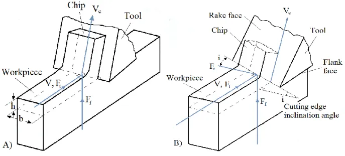
Figure 2-1: A) Orthogonal and B) oblique cutting process geometries……… 4
Figure 2-2: Orbital drilling………... 5
Figure 2-3: K2X10 Huron® high-speed machining center………... 5
Figure 2-4: Two allotropic forms of titanium……….. 8
Figure 2-5: Typical reinforcement types………..….. 10
Figure 2-6: Lay-up laminate………..………. 11
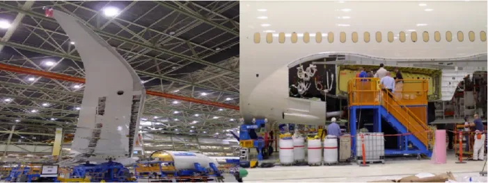
Figure 2-7: Boeing 787 Dreamliner……….……12
Figure 2-8: Assembling of the Boeing 787 Dreamliner; CFRP/Ti stack is used in the wing-fuselage connection………..…… 13
Figure 2-9: multi-material stacks machining issues leading to low tool life………..……. 13
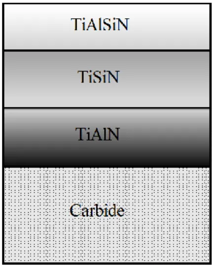
Figure 2-10: Layer structures of the TiAlSiN/TiSiN/TiAlN coatings……...…………..……...… 14
Figure 2-11: Photos of four flutes carbide end mill with TiAlSiN/TiSiN/TiAlN coatings……… 15
Figure 2-12: Types of tool wear….……… 16
Figure 2-13: Typical tool wear stages…………..……….. 17
Figure 2-14: Characterization of flank wear and crater wear.……… 18
Figure 2-15: Koch curve formation..……….. 21
Figure 2-16: Three different size grids for Great Britain……… 23
Figure 4-1: Experimental setup……….. 29
Figure 4-2: Cutting forces (top), total cutting force (𝐹𝑇) (bottom) during the first hole drilling… 31 Figure 4-3: The stable part of total cutting force (𝐹𝑇) during titanium machining from Figure 4-2, which is divided into three equal sections (A, B, C) for the first hole drilling….……….. 32
Figure4-4: Evolution of total cutting force average along hole drilling…….……… 33
Figure 4-5: The total cutting force signal through the tool life during the first, eighth, twelfth, and twentieth hole drilling in the complete sections A, B and C (with magnification areas)………… 34
Figure 4-6: Regularization analysis graph(𝑙𝑜𝑔 𝑙𝑎 vs 𝑙𝑜𝑔 𝑎) in all sections (A, B, C)……… 37
Figure 4-7: Tool wear stages in a normal cutting situation………. 38
Figure 4-8: Photos of tool along the tool life after drilling of eight, twelve and twenty holes…... 39
Figure 4-9: Evolution of the tool wear VBmax vs the hole drilled……… 40
Figure 4-10: The fractal dimension through the tool life for all sections (A, B, C)……… 41
Figure 4-11: The topothesy (𝐺) vs the holes drilled……… 42
Figure 4-12: The coefficient of determination (𝑅2) vs the holes drilled……… 42
Figure 4-13: The fractal index ( 𝐼) vs the holes drilled………...……… 43
LIST OF SYMBOLS AND ABBREVIATIONS
AE Acoustic emissionBCC Body-centered cubic
CFRP Carbon fiber reinforced plastics D Fractal dimension Ff Feed force Fr Radial force Ft Tangential force FT Resultant force HCP Hexagonal close-packed R2 Coefficient of determination VBB Average flank wear width VBmax Maximum flank wear width
CHAPTER 1
INTRODUCTION
1.1 Motivation
Titanium alloys are widely used in the aerospace industry and the utilization of hybrid structures made of composites and of titanium alloys is increasing. These materials exhibit excellent mechanical properties, including high stiffness, high corrosion resistance, and high tensile strength with low weight, but machining of these multi-material stacks is challenging due to the combination of diverse wear mechanisms which accelerate tool wear. Recent research has studied machining of the hybrid stacks to provide industry requirement, but it has only focused on the analysis of the cutting force and acoustic emission signals of composite parts while machining hybrid stacks; information from the machining of homogenous materials involved in multi-material stacks may have been missed. This study is focused on the analysis of the signal from orbital drilling of the titanium alloy within carbon fiber reinforced plastics (CFRP) with Ti-6Al-4V titanium alloy stack.
1.2 Research objectives
The main objective of this study is to analyze the cutting force signals from machining of titanium alloys within CFRP/Ti stack to improve online tool wear monitoring and estimate tool life. The secondary objective is to introduce new statistical parameters based on the fractal analysis of cutting force signals in order to monitor and estimate tool wear evolution, and to propose a limit criterion to prevent low machining quality in place of long machining tests.
1.3 Hypothesis statement
1. The fractal dimension is related to the irregularity and complexity of a fractal and it can be used to describe the non-linear behaviour of signals and extract some aspects of signals.
2. The maximum tool wear (VBmax) is used to evaluate tool life as, it is an accepted measure for assessment of the tool wear (ISO.3685, 1993).
1.4 Assumption
1. During the machining of a stack of CFRP/Ti, the main tool wear mechanism is abrasion due to the toughness of the carbon fibers; however, adhesion, chipping, attrition and abrasion are also expected (Çalışkan, Kurbanoğlu, Panjan, Čekada, & Kramar, 2013; Pramanik & Littlefair, 2014; Rimpault, X., Chatelain, Klemberg-Sapieha, & Balazinski, 2016).
2. Orbital drilling is used because it often leads to lower thrust force, smaller burrs, and less fiber delamination in composites, as compared with axial drilling (Wang, Qin, Ren, & Wang, 2011).
CHAPTER 2
LITERATURE REVIEW
2.1 Machining
Metal cutting is a large part of machining, which involves a relative motion between the tool and workpiece to remove unwanted material. Orthogonal and oblique cutting are two basic types of metal cutting processes which will be explained in this section.
2.1.1 Orthogonal cutting
Orthogonal cutting is a type of machining in which material is removed using a defined tool cutting edge which is perpendicular to the direction of tool motion. Orthogonal cutting is also known as two-dimensional plane cutting because the cutting forces can be represented by 2D coordinates. As shown in Figure 2-1, the cutting forces are exerted in the direction of velocity (Ft) and the direction of uncut chip thickness (Ff) and the resultant force (FT) is calculated as follows:
FT = √Ft2 + Ff2 (2.1) Where Ft is tangential force and Ff is feed force.
2.1.2 Oblique cutting
The main difference between orthogonal cutting and oblique cutting is that in the oblique cutting the tool cutting edge makes an angle (i) other than a right angle with respect to the direction of motion. Oblique cutting is also called three-dimensional plane cutting, and the additional third force is exerted in the radial direction (Fr). The resultant force (FT) is also calculated using:
Figure 2-1: A) Orthogonal and B) oblique cutting process geometries (Altintas, 2012)
2.1.3 Orbital drilling
Drilling is an important methods of machining in the aerospace industry. For a single aircraft, between 100,000 and 1,000,000 riveting holes are drilled. Orbital drilling, which is also called helical milling in the literature, is a machining process in which the tool has helical movement through the material, as shown in Figure 2-2. For difficult-to-cut materials like Ti alloys, orbital drilling offers advantages over axial drilling; for instance, it does not require disassembly to remove chips, deburr, or clean coolant or lubricants. Moreover, orbital drilling decreases burr size, reduces composite delamination during machining of composite materials, and diminishes cutting forces. Moreover, one tool diameter may be suitable for different holes to be machined (Denkena, Rehe, Nespor, & Dege, 2011; Pereira, Brandão, de Paiva, Ferreira, & Davim, 2017). In this study, orbital drilling was performed on the K2X10 Huron® high-speed machining center (Figure 2-3) with a dust extraction system which was mounted onto the machine for the sake of health and safety and the technical specification of this machine is also presented in Table 2-1.
Figure 2-3: K2X10 Huron® high-speed machining center Figure 2-2: Orbital drilling of CFRP/Ti stack
Table 2-1: Technical specification of K2X10 Huron® high-speed machining center
Machine type 3-axis High speed CNC machine
Manufacturer Huron Graffenstaden
Year of manufacture 2007 Controller Siemens 840 D Spindle 28 000 TPM, 20.9 Nm [185lbs-in] Number of tools 20 Displacements 1000 x 800 x 500 mm – [39.4 x 31.5 x 19.7 in] Capacity 1150 X 800 mm, 1000 kg – [45.3 X 31.5 in, 2200 lbs]
Cutting speed 60 m/mn – [2362 in/min]
Feed rate 30000 mm/min – [1181 in/min] @ 6m/s2 and
150m/s3
2.2 Titanium alloys
Titanium alloys are highly attractive for the aerospace industry because they perform well in the aerospace environment as a consequence of remarkable properties such as high specific strength, high corrosion resistance and high fatigue resistance. Due to the high strength-to-weight ratio, these alloys are used in aircraft engines and support structures. These alloys also have the ability to maintain their high strength at elevated temperatures, explaining their usefulness as engine component materials(Jianxin, Yousheng, & Wenlong, 2008). These alloys are also utilized in other industries, e.g. medical, automotive, offshore, chemical and petroleum industries, in which the
machined components need good surface integrity and dimensional accuracy (Safari, Sharif, Izman, & Jafari, 2014).
However, the machinability of titanium alloys is poor and these alloys are considered difficult-to-machine materials. Yang and Liu indicated some reasons for the poor machinability of titanium alloys (Yang & Liu, 1999):
1. Low thermal conductivity: The poor thermal properties of titanium for machining cause the temperature at the tool-workpiece interface to increase. The tool edge temperature easily reaches 1000 ℃, so the tool life decreases.
2. Very thin and long, stringy chip: When the chip is very thin, the contact area between the tool and chip is small. With the low thermal conductivity of titanium, the stress on the tool tip increases, so the tool wear rate increases. Moreover, the high strength of titanium at elevated temperatures opposes the plastic deformation needed to form a chip. A long, stringy chip will be produced, which is difficult to handle.
3. High chemical affinity: Titanium has a strong affinity to almost all the tool materials at elevated temperatures; hence, it accelerates the tool wear and causes chipping and a premature end to useful tool life.
4. Low elastic modulus: The low modulus of elasticity of titanium, and consequent high thrust force can cause significant deflection of the workpiece.
5. Sparks: Titanium has a tendency to ignite during machining and sparks are noticed because of the high temperature.
2.2.1 Classification
Basic knowledge of titanium and its alloys can help to better understanding the machining of these materials. Titanium alloys are classified into four categories which is summarized fromreferences (Nguyen & Kwon, 2014; Sha & Malinov, 2009; Yang & Liu, 1999):
1. Unalloyed (commercial purity): unalloyed titanium has very limited applications because of the low strength, but it has excellent corrosion resistance.
2. Alpha (α or hexagonal closed packed (HCP) is shown in Figure 2-4 ) and near-α: 'α stabilizers' such as Al, O, N, Ga, and C produce an increase in the temperature of the
allotropic transformation, and α alloys such as Ti5Al2.5Sn and Ti8Al1Mo1V have superior creep resistance, high corrosion resistance and good weldability. Alpha alloys are utilized for high temperature applications, but they are not heat-treatable and they are brittle with low to medium tensile strength.
3. Beta (β or body-centered cubic (BCC) is shown in Figure 2-4): The 'β stabilizers' such as Ta, Mo, V (isomorphous formers), Cu, Mn, Fe, Ni, Co, Cr and H (eutectoid formers) produce a decrease in the transformation temperature. Beta alloys such as Ti11.5Mo6Zr4.5Sn and Ti5553 have higher strength and higher toughness than the α and the α − β alloys, but they have the poorest machinability. Furthermore, segmented chips, the plastic instability and catastrophic thermoplastic shear in the primary shear zone are drawbacks when machining β alloys.
4. α – β: 70% of all titanium used is α – β alloy, and these alloys contain both α stabilizers and β stabilizers, such as Ti6Al4V and Ti5Al4V. Their properties are different, but it is generally acknowledged that they have high strength at room temperature and moderate strength at high temperature. In addition, the chip segmentation frequency in α − β alloys are higher than that in α alloys and lower than that in β alloys.
2.2.2 Ti-6Al-4V
Ti-6Al-4V is the most widely used titanium alloy and it comprises up to 60% of the total titanium production(Nguyen & Kwon, 2014). This alloy has widespread use in the surgical, chemical, aerospace and shipbuilding industries, as a consequence of outstanding corrosion resistance, a high strength-to-weight ratio, and good toughness. Physical and chemical properties of this alloy are presented in Table 2-2 and chemical composition of this alloy also is presented in Table 2-3. (Nguyen & Kwon, 2014; Rao & Shin, 2002).
Table 2-2: Physical and chemical properties of Ti6Al4V alloy (Cardarelli, 2008).
Density (𝛒 𝐤𝐠. 𝐦⁄ −𝟑) 4420
Ultimate tensile strength (𝛔𝐔𝐓𝐒⁄𝐌𝐏𝐚) 897–1205
Young modulus (𝐄 𝐆𝐏𝐚⁄ ) 106-114
Brinell hardness (HB) 330
Melting range (°C) 993
Table 2-3: Chemical composition of Ti-6Al-4V titanium alloy (Fan, Sun, Meng, Gao, & Tong, 2009)
Al V Ti Fe Si C N H O Others
2.3 Composite materials
2.3.1 Generalities
A composite material is made by combining two or more materials in order to improve the chemical, physical, and mechanical properties. Composite materials commonly consist of two components: reinforcement and matrix. The hardest and strongest part of the composite is reinforcement which is generally a fiber or a particulate. The strength and stiffness of the composite are provided by the reinforcement, and the maintenance and protection of the fibers from abrasion is provided by the matrix. The matrix can be a polymer, metal, or ceramic. Particulate composites are cheaper than fiber composites, but usually they are much weaker because they contain less reinforcement. Fibers are also divided into two groups: continuous fiber and discontinuous fiber. The examples of continuous and discontinuous fibers are shown in Figure 2-5. Continuous fibers have a preferred orientation, as in unidirectional fiber composites; discontinuous fibers have random orientations, as with
chopped fibers. Generally, higher strength can obtained with smaller diameter fibers, which is more expensive (Campbell, 2010). Polymer matrices are classified according to two categories: thermosets and thermoplastics.
During thermoset
manufacturing, resins are cured into a solid form and they cannot be reprocessed and returned to their original form. Conversely, thermoplastic polymers are manufactured by heating above the resin’s
melting temperature and can be melted and remolded.
2.3.2 Advantages and disadvantages of composite materials
Composite materials have lighter weight than metallic materials, and their fatigue lives and stiffnesses are also improved. In addition, they have high corrosion resistance, high specific strength and high specific modulus. They can reduce assembly costs by bonding detail parts together to make an integrated part. In spite of the good properties of composite materials, there are some disadvantages like high raw material cost and high fabrication cost, and the probability of delamination or ply separation during machining. Moreover, the strength in the out-of-plane direction is poor, and repairing composite structures is more difficult than in metallic structures (Campbell, 2010).
2.3.3 CFRP
The utilization of carbon fiber reinforced plastic (CFRP) is increasing in the aerospace industry as a consequence of high strength-to-weight ratio and low weight. CFRP consists of two different materials: carbon fibers and a matrix. The matrix in CFRP is a thermoset resin which is the epoxy resin in this study. CFRP has laminated structure which is anisotropic material and the properties of the material depend on the direction of the plies. The CFRP is manufactured by manual lay-up which is shown in Figure 2-6 and afterwards cured in an autoclave (Rimpault, Xavier, 2016).
2.3.4 CFRP/Ti stack
One of the innovative structural configurations in the aerospace industry is a multi-material stack, especially hybrid structures made of carbon fiber reinforced plastics (CFRP) and lightweight metals such as titanium alloys (Ti-6Al-4V). CFRP has limited structural
loadbearing capability and low wear resistance, so to improve specific characteristics such as wear resistance and elastic modulus without increasing the weight, titanium sheets are stacked with CFRP (James & Sonate, 2017). Utilization of these kind of hybrid stacks enables aerospace manufacturers to enhance resistance and specific characteristics without significantly increasing the weight. These hybrid stacks have good mechanical properties like high strength, high corrosion resistance and high stiffness with low weight, which are all essential attributes for aerospace (Pecat & Brinksmeier, 2014). Many aircraft manufacturers such as Boeing, Airbus, Bombardier, etc., have employed hybrid structures to improve the characteristics of this new-generation structures. For instant, CFRP/Ti stack is used in the wing and the fuselage connection of the Boeing 787 Dreamliner (Figure 2-7). The area where the wing is joined to the fuselage is made of a titanium alloy and the wing is made of carbon fiber reinforced plastics which is shown in Figure 2-8 (Xu & El Mansori, 2016).
Despite the great properties of multi-material stacks, it is challenging to machine these materials while meeting the desired quality because the combination of the different wear mechanism can accelerate the tool wear rate which is presented in Figure 2-9 (Isbilir & Ghassemieh, 2013). Chipping, abrasion, adhesion and attrition are the tool wear mechanism during machining of CFRP/Ti stack, but the main tool wear is abrasion due to the toughness of the carbon fibers (Pramanik & Littlefair, 2014; Rimpault, X., Chatelain, Klemberg-Sapieha, & Balazinski, 2017).
Figure 2-8: Assembling of the Boeing 787 Dreamliner; CFRP/Ti stack is used in the wing-fuselage connection (Paur, 2009, February 13)
Figure 2-9: multi-material stacks machining leading to low tool life (Xu & El Mansori, 2016) CFRP machining
-
Anisotropic behavior- Abrasive nature
- Low thermal conductivity
Titanium alloy machining - Low thermal conductivity - Strong chemical affinity to tool materials
CFRP/Ti stack machining - Poor machined surface quality
2.4 Tool
Carbide tools are used in machining of hard materials due to their high toughness, hot hardness and low cost but their tool wear rate is high which limits the utilization of these kinds of tools. The only solution to increase machinability with carbide tools is to protect the tool with appropriate coatings (Çalışkan et al., 2013). Generally, coating material needs to have some properties to obtain an acceptable lifetime, such as high hardness, low friction coefficient, low thermal conductivity and high adhesion to the cutting tool surface. In addition, combinations of coatings as multilayer designs leads to superior properties like higher microhardness (Caliskan, Celil, & Panjan, 2016). Multilayer TiAlSiN/TiSiN/TiAlN coatings are deposited on carbide cutting tools in this study and it is shown in Figure 2-10. This experimental coating is smooth and chemically stable with low residual stresses, and its maximum operating temperature is 1100 ℃ (Çalışkan et al., 2013). Caliskan et al. drew a comparison between four types of hard coatings: AlTiN/TiN, TiAlSiN/TiSiN/TiAlN, TiN and TiAlN coatings, which are deposited on carbide milling inserts during steel milling. He indicated that the TiAlSiN/TiSiN/TiAlN coating has the highest hardness and is the most resistant to plastic deformation among the investigated coatings. The AlTiN/TiN demonstrates superior performance in scratch tests and has better adhesion to the substrate and the longest lifetime. By comparison, TiN has the lowest wear rate
(Çalışkan et al., 2013). Caliskan et al. also reported that the TiAlSiN/TiSiN/TiAlN coating can enhance the wear resistance of carbide cutting tools and has higher wear resistance and longer lifetime than TiN and TiAlN coatings during steel milling (Caliskan et al., 2016). In this study, the tool is a four flutes carbide end mill with TiAlSiN/TiSiN/TiAlN coatings, with a 4 mm diameter, 30° helix angle and 11 mm maximum depth of cut which is shown in Figure 2-11.
Figure 2-10: Layer structures of the TiAlSiN/TiSiN/TiAlN
Figure 2-11: Photos of four flutes carbide end mill with TiAlSiN/TiSiN/TiAlN coatings
2.5 Tool wear
Tool wear is a significant challenge in machining. Tool wear increases cutting force and temperature and decreases the surface quality and accuracy of finished parts. Tool wear depends on several parameters, including tool geometry, tool material, workpiece material, cutting speed, feed, depth of cut, coolant and lubricant, and the characteristics of the machine. Generally, tool failure and wear are classified into two groups: premature tool failure and progressive tool wear. Premature tool failure often occurs when the cutting edge breaks because of the rapid growth of the crater wear or pre-existing cracks in the tool, and this tool edge breakage leads to failure of the tool (Cheng, 2009). On the other hand, progressive tool wear is always used to define the useful tool life. It consists of crater wear and flank wear. Figure 2-12 depicts some types of wear and failures which commonly occur on the cutting tool.
Figure 2-12: Types of tool wear: 1. flank wear, 2. crater wear, 3. plastic deformation, 4. built-up edge, 5. edge chipping or frittering, 6. gross fracture, 7. comb (thermal) cracks, 8. chip
hammering (Stephenson, 2006)
As seen in Figure 2-12, number 1 illustrates flank wear, which occurs in the tool flanks where the tool has contact with finished surface. Flank wear most commonly results from abrasion of the cutting edge (Stephenson, 2006). Flank wear can increase the total cutting force and surface roughness of the component and it can decrease the dimensional accuracy of finished parts. Flank wear can be reduced by raising the abrasion and deformation resistance of the tool material and by using appropriate tool coatings.
Number 2 shows crater wear, which happens on the tool rake face as a result of chip flow. Diffusion and chemical wear are the main causes of the crater wear. Moderate crater wear does not affect tool life, but excessive crater wear can cause deformation or fracture of the tool. Reducing the cutting speed and using an appropriate coating can mitigate crater wear (Stephenson, 2006). Number 3 illustrates plastic deformation at the tool tip. When the temperature at the tool tip increases, the tool tip softens, loses its hardness, and deforms plastically. Poor selection of tool material and cutting conditions are the main reasons for plastic deformation, resulting in loss of dimensional accuracy, severe flank wear and poor surface finish (Stephenson, 2006).
Built-up edge formation is illustrated in number 4. Built-up edges occur when the temperature and pressure at tool chip interference increase and metal adheres to the cutting edge; after some time, a built-up edge forms. This is especially common during machining of soft metals like aluminium
alloys. Low cutting speeds can promote the formation of built-up edges, which can cause tool chipping and poor surface quality (Stephenson, 2006).
Edge chipping and gross fracture are illustrated in numbers 5 and 6, respectively, which can lead to tool breakage. In continuous cutting, as with turning, fracture or chipping are rare, but in interrupted cutting like milling these kinds of wear are common. De Melo et al. indicated the main cutting parameter which has an effect on tool chipping or fracture is feed rate (De Melo, Milan, Da Silva, & Machado, 2006).
Cracks can appear on the rake or flank faces because of the cyclical heating and cooling during cutting, especially in interrupted cutting. After a certain number of cycles, thermal cracks transform into comb cracks, as is shown in number 7.
Improper chip control can cause chips to curl back and touch the tool face, which leads to chipping of the tool surface, called chip hammering. Hammering is shown in number 8. Chip hammering can be mitigated by changing the lead angle, feed rate, depth of cut, or tool nose radius (Stephenson, 2006).
As shown in Figure 2-13, the flank wear rate changes with time in a typical cutting situation and it is divided into three stages. In the initial or primary wear stage, the tool wears rapidly due to the high pressure in the small contact area. After initial tool wear, flank wear increases slowly at the steady state wear stage until it reaches the third, accelerated wear stage in which wear accelerates and becomes severe, rapidly leading to tool failure in this final stage.
2.5.1 Tool wear specification
Tool wear can be measured using crater wear on the rake face and flank wear on the flank face. On the flank face, the average (VBB) and the maximum (VBBmax) values of the flank wear width which are shown in Figure 2-14 are usually measured and the major cutting edge is divided into three zones: C, B, and N. Zone C is the curved part of the cutting edge and zone N is the quarter of the worn cutting edge from the tool corner and zone B is the remaining straight part between C and N. Similarly, on the rake face, the crater width (KB), crater depth (KT) and the crater center distance (KM) are the values normally measured. On the flank face, the amount of material worn off can be approximated by:
vw = VBB2∗b∗tanθ
2 (2.3) Where b is the cutting width and θ is the relief angle.
On the rake face, the total amount of crater wear can be approximated similarly: vcr =
2b(KB−KF)KT
3 (Stephenson, 2006)(2.4)
2.5.2 Tool wear monitoring
Tool wear monitoring is a significant aspect of advanced manufacturing, and prediction of tool life plays an important role in improving manufacturing processes. Hidayah et al. indicated that tool condition monitoring can allow for cutting process speed to be increased by 10% to 50% and decrease costs by 10% to 40% (Hidayah, Ghani, Nuawi, & Haron, 2015). Jantunen listed a number of reasons for the importance of tool condition monitoring including the possibility of unmanned production, obtainment of required surface qualities, and means to save on time and expenses (Jantunen, 2002). Generally, tool wear monitoring methods are classified into two categories: the direct and indirect methods. The direct method is an offline method which estimates tool wear directly based on surface textures, using sensors of various kinds, such as radioactive, optical, laser scan micrometer, and electrical resistance sensors (Stephenson, 2006). The indirect method is utilized to analyze signals of cutting force, vibration, acoustic emission (AE), among others. Such signals are acquired during the machining process in order to monitor the tool condition in real time and estimate the tool wear. Moreover, the indirect or “online” tool wear monitoring method is playing an important role in current engineering in order to meet the customer’s requirements and reduce production costs. So, this method has been appealing to researchers (Jantunen, 2002). Generally, tool condition monitoring follows the following steps. Several process variables, including cutting forces, acoustic emission, vibration, temperature, surface finish, and noise, are sensitive to cutting tool condition and to machining parameter values. These variables are acquired by appropriate sensors. The acquired signals are then processed by a variety of methods including neural networks (Elforjani & Shanbr, 2018), fuzzy logic (Ren, Baron, Balazinski, Botez, & Bigras, 2015), genetic algorithms (Pandiyan, Caesarendra, Tjahjowidodo, & Tan, 2018), or fractal analysis (Rimpault, X. et al., 2016) in order to generate decision making systems able to provide diagnoses of manufacturing issues. Notably, Teti et al. surveyed the literature on tool condition monitoring and produced a comprehensive survey of sensor technologies, signal processing, and decision making strategies for process monitoring (Teti, Jemielniak, O’Donnell, & Dornfeld, 2010).
2.6 Fractal analysis
B.B. Mandelbrot, an American scientist, coined the word ‘fractal’ in the mid-1970s to characterize the length of the British coastline. Fractals are irregular objects and cannot be classified as geometric figures. Fractals have some form of self-similarity and affine structure and they have fractal dimension which is greater than topological dimension (Mandelbrot, 1982).
Fractal theory is becoming a strong tool for the analysis and prediction of the behaviour of complex dynamic systems and it can be applied in fields such as chemistry, physics and geology (Chuangwen & Hualing, 2009).
2.6.1 Fractal dimension
Fractal dimension characterizes the irregularity and complexity of a system with a single value. The fractal dimension is expressed by:
D = lim ε→0 ln N(ε) ln(1 ε) (2.5) Where N(ε) is the number of pieces (self-similar pieces) and ε is a scaling factor. To clarify the definition of the fractal dimension, let us consider one of the most famous fractal objects, the Koch flake.
Construction of the Koch curve is shown in Figure 2-15; a straight line is chosen and broken into three equal parts, then central part is removed and replaced by the two other segments. In the next step, the same operation is repeated for each straight part. After infinite repetition, the Koch curve will be obtained. This curve is self-similar and the dimension of the curve is constant at all scales. The fractal dimension of the Koch flake is calculated as follows:
D = lim k→∞ ln N(k) ln(1 εk) = lim k→∞ ln 4k ln 3k = 1.2619 (2.6)
Where N is the number of pieces at the first stage with the length of ε =1
3 and after k stages, the number of pieces is N(k) = 4k and the length measurement is ε
k= 1
3k ,so the fractal dimension of the Koch curve is approximately 1.26 (Sahoo, Barman, & Davim, 2011).
Figure 2-15: Koch curve formation (Sahoo et al., 2011)
2.6.2 Fractal analysis techniques
Fractal dimension can be estimated using numerous techniques such as correlation analysis, information analysis, regularization analysis, box-counting analysis and so on. However, all of these methods follow three steps, summarised as follow:
1.
A property of an object is evaluated at different scales.2.
A logarithmic graph (log(measured quantities) vs log(step sizes)) is plotted and the least-squares regression line is fitted through the points.3.
Fractal dimension, which is the slope of the regression line, is calculated (Lopes & Betrouni, 2009).Three fractal analysis methods will be explained briefly in this chapter. The regularization analysis chosen for this study was selected for its relatively good repeatability rates in recent papers (Feng, Zuo, & Chu, 2010; Rimpault, X. et al., 2016).
2.6.2.1 Regularization analysis
Regularization dimension measures the “roughness” and irregularity of a signal. Signals are regularized/smoothed by convolution with different kernels (ga) with a width of a.
Let fa be the convolution of f with ga.
fa=f ∗ ga (2.7)
So, la (the length of fa) approaches to infinity as a (kernel’s width) tends to 0 and D (the regularization dimension) measures the speed of this conversion, itself calculated with:
D = 1 − lim a→0
log la
log a (2.8) When the coefficient of determination R2 of the linear regression of a part of the curve ( log 𝑙𝑎 vs log 𝑎 ) is close to 1, the fractal dimension is calculated (Rimpault, X. et al., 2016).
2.6.2.2 Box counting method
The box counting method is the most frequently used method to estimate the fractal dimension. Small boxes with adjustable size are used to cover a fractal and the fractal dimension can be calculated using: D = lim ε→0 log N(ε) log(1 ε) (2.9) where N(ε) is the number of boxes and ε is the box size, usually the straightest part of the curve of log N(ε) vs log (1
ε) used to calculate the box counting dimension. For example, the length of a coastline can be estimated in the map by using different size of grids based on box-counting method as shown in Figure 2-16 and it was calculated by Eq. (2.9) as given in the Table 2-4. Lopes et al. indicated that this method has many limitations like; it needs signal binarization, and if the signal is statistically self-similar, this method can be reliable (Lopes & Betrouni, 2009).
Figure 2-16: Three different size grids for Great Britain (Mandelbrot, 1982)
Table 2-4: The length of a coastline (Duong, 2015)
N (𝛆) 𝛆 (km) L (km) 6 500.00 3000 12 258.82 3106 24 130.53 3133 48 65.40 3139 96 32.72 3141 192 16.36 3141
2.6.2.3 Correlation fractal analysis
Correlation analysis is one of the widely used methods to calculate fractal dimension of the curve. A set of vectors from the time series is extracted as follows:
x1 = {x(1), x(1 + τ), … , x(1 + (M − 1)τ)} (2.10) x2 = {x(1 + k), x(1 + k + τ), … , x(1 + k + (M − 1)τ)}
(...)
xN+1 = {x(1 + Nk), x(1 + Nk + τ), … , x(1 + Nk + (M − 1)τ)} Where x(t) is the discrete time series signal, N is number of vectors, M is the phase space, k is the space between the vectors and τ is the space between two points.
The correlation function c(ε) is calculated using:
c(ε) = 1 N(ε)(N(ε)+1)∑ ∑ θ(ε − |xi− xj|) N+1 j=1 N+1 i=1 , j ≠ i, (2.11) where xi and xj are the position vector on the attractor and θ is the Heaviside step function; θ(x) = 0 if x ≤ 0 and θ(x) = 1 if> 0.
Then, the correlation dimension can be estimated as a derivative of the correlation function: D = lim
ε→0 log c(ε)
log ε (2.12) The correlation dimension is the slope of the straight line portion of the graph of log c(ε) vs log ε (Logan & Mathew, 1996).
CHAPTER 3
STRUCTURE
Chapter 1 presented the motivation for the work, its objectives, assumption and the hypotheses made. The motivation for this study is to ply the unexploited information from signals obtained during machining of the homogenous materials involved in multi-material stacks. The principle objective is to analyze the cutting force signals while machining titanium alloys within CFRP/Ti stack in order to improve online tool wear monitoring and tool life estimation.
The literature review in Chapter 2 introduced the state of the art in the machining, the material, and the tooling, and presented an introduction to the analysis techniques used in this study.
The general structure of the work follows here. Also included is an article introduction.
The subsequent chapter consists of the article “Tool wear monitoring based on fractal analysis of cutting force signals while machining titanium alloy within CFRP/titanium stack,” which was submitted for peer review for publication in the Journal of materials processing technology. That article is the core of this study. The fractal analysis of cutting force signals acquired during machining of titanium alloys within CFRP/Ti stack is a useful technique for the characterization of signal features. Such analysis may well find a key role for the prediction of tool wear. In this study, the irregularity and “roughness” of the total cutting force signals of the titanium alloy are characterized in terms of fractal dimension while drilling of a stack of carbon fiber reinforced plastics (CFRP) and Ti-6Al-4V titanium alloy. The fractal dimension (D), the topothesy (G) and the coefficient of determination (R2) based on regularization analysis of the total cutting force signal during titanium machining are calculated in order to identify distinct wear stages and enable estimation of the tool wear. The empirical fractal index is also introduced as a statistical parameter in order to monitor and estimate the tool wear, as a replacement for long machining tests. In conclusion, fractal analysis of cutting force signals can be used to monitor the tool wear during titanium alloy machining involved in CFRP/Ti stack and the results show great potential for further development.
This master thesis ends with a general discussion and conclusion to sum up its original contributions.
CHAPTER 4
ARTICLE 1: TOOL WEAR MONITORING BASED ON
FRACTAL ANALYSIS OF CUTTING FORCE SIGNALS WHILE
MACHINING TITANIUM ALLOY WITHIN CFRP/TITANIUM STACK
Maryam Jamshidi
1, Xavier Rimpault
1,2,*, Marek Balazinski
1, Jean-François
Chatelain
21 Department of Mechanical Engineering, Polytechnique Montréal, 2900 Édouard-Montpetit Blvd., Montreal, QC, H3T 1J4, Canada
2 Department of Mechanical Engineering, École de technologie supérieure, 1100 Notre-Dame St W, Montreal, QC, H3C 1K3, Canada
* Submitted to Journal of materials processing technology in February 2018.
4.1 Abstract
In the aerospace industry, the utilization of hybrid structures made of composite and lightweight metals is increasing. Machining stacks remains challenging and its process needs to be optimized and monitored closely. Cutting force signals are one of the most significant indicators to be considered in online tool condition monitoring. Recent research has focused on the analysis of the cutting force or acoustic emission signals of composite parts during machining of the hybrid stacks; in contrast, useful information in the signal from the machining of homogenous materials has been missed. In this context, the fractal analysis of those signals acquired during the titanium alloys machining is a useful technique for thecharacterization of signal features, and has a key role in predicting tool wear. In this study, the irregularity and “roughness” of the total cutting force signals of the titanium alloy are characterized in terms of fractal dimension during orbital drilling of a stack of carbon fiber reinforced plastics (CFRP) and Ti-6Al-4V titanium alloy. Fractal parameters are found to be adequate for the identification of distinct wear stages and prevent low machining quality.In addition, a fractal index is proposed as a statistical parameter to monitor tool wear during titanium alloy machining to mitigate the need for long machining tests and to improve the monitoring process.
4.2 Introduction
Titanium alloys are extensively used in the aerospace industry. Titanium alloys offer good mechanical properties such as high strength to weight ratio, high tensile strength, high fatigue resistance, low mass density and also high corrosion resistance. Titanium alloys are used in many aircraft components, including structures, gas turbine engines, and non-structural applications such as aircraft flooring, tubes or pipes. These alloys are also attractive for other industries, e.g. chemical, automotive, offshore and petroleum industries as well as medical purposes [1]. Notwithstanding their good properties, titanium alloys are considered difficult-to-machine materials. The low thermal conductivity of titanium alloys leads to elevated cutting tool
temperature. Moreover, tool life decreases because of the extreme affinity of titanium alloys to many tool materials. As a result, the tool wear rate and the machining costs are high, and low productivity is expected. The hardness of titanium causes the force and stress to increase rapidly on the cutting edge [2].
The use of hybrid structures made of carbon fiber reinforced plastics (CFRP) and lightweight metals such as titanium (Ti) or aluminum is increasing in the aerospace industry and researchers have been working on the machining of composite and metal stacks. Among the available hybrid stacks, CFRP/Ti is one of the most popular ones due to excellent mechanical properties like high stiffness, high corrosion resistance with low weight and high tensile strength, but in the assembly process, drilling of this stack is challenging [3]. Adhesion, chipping, attrition and abrasion are the tool wear mechanisms during machining of CFRP/Ti stacks. However, the main tool wear
mechanism is abrasion due to the toughness of the carbon fibers [4, 5]. During drilling of titanium, Zhang et al. determined that about 90% of the plastic deformation is converted into heat, and because of the low thermal conductivity of titanium, hence a large portion of generated heat is absorbed by the tool and the tool fails quickly [1].
In this study, instead of axial drilling, orbital drilling was used. Orbital drilling is a machining process in which the tool follows an helical movement through the material and often leads to lower thrust force, lower burr size and less fiber delamination in composites [6].
Rimpault et al. analyzed the cutting force and acoustic emission signals during CFRP machining while orbital drilling of the stack of CFRP/Ti, but analysis of the cutting force signals during titanium machining was omitted and some potential information may have been missed [4]. For the current paper, the total cutting force signals of titanium machining during orbital drilling of
the CFRP/Ti stack is analyzed. Due to the high sensitivity of the cutting force signals to change of cutting states, monitoring of cutting forces has been used in recent years [7-11]. Tool wear causes alteration of the contact area between the tool and the workpiece, and thus evolution of the cutting force signals.
In order to control and optimize manufacturing processes, tool condition monitoring can be efficient to predict continuous tool wear processes. Hidayah et al. indicated that tool condition monitoring can allow for cutting process speed to be increased by 10% - 50% and principally decrease cost by 10% to 40% [7]. Generally, tool wear monitoring methods are classified into two categories: the direct and indirect methods. Direct methods, such as visual inspection, are performed offline and assess tool wear directly, but currently, manufacturing industries need an online system to monitor the tool wear in order to meet customer requirement and reduce production costs. Such a system may help prevent tool breakage upon the costly workpiece during machining and aid in replacing the worn tool at the end of its effective lifetime. Hence, the indirect or online methods have been appealing to researchers. Indirect methods imply
monitoring of tool condition in real time with the help of signals which are acquired during the machining process [12].
In this work, an indirect method of tool wear monitoring was used to predict the tool wear evolution based on analysis of the total cutting force signals. Rimpault et al. found that during composite machining, parameters calculated from the acoustic emission signal analysis are more efficient than the cutting force signals to estimate the tool wear [4]; nevertheless, for homogeneous materials, especially titanium alloys, analysis of the cutting force signals could be adequate. The research herein focuses on the titanium machining within the CFRP/titanium stack in order to fit as possible to industrial processes.
4.3 Experiment and data set
A stack of a quasi-isotropic carbon fiber reinforced plastics (CFRP) and Ti-6Al-4V titanium alloy was used. Orbital drilling was performed on the K2X10 Huron® high-speed machining center with a dust extraction system which was mounted onto the machine for the sake of health and safety. The hole diameter was 5.85 mm and the drilling was performed until tool breakage and 20 holes were achieved. The cutting parameters and detailed information about the cutting tool are presented in Table 4-1. The cutting conditions were set after preliminary experiments. The input signal was acquired using an amplifier and a data acquisition system at a 48 kHz sampling rate. The cutting force was acquired by a dynamometer table during the drilling of CFRP with a 3.3 mm thickness at the top of the stack and Ti-6Al-4V with a 3.0 mm thickness at the bottom. The schematic of the setup is presented in Figure 4-1. The photos of the tool were recorded by VHC 600+500F Keyence® optical microscope, which were used to estimate the tool wear. The maximum tool wear is the average of the maximum tool wear on each of the four cutting edges of the tool. The average of the four cutting edge tool wear evaluation gives the (VBmax) displayed hereafter.
Table 4-1: Tool specifications and cutting parameters Cutting Tool
Type Four flutes carbide end mill
Diameter 4 mm
Helix Angle 30°
Maximum Depth of cut 11 mm
Cutting Parameters Feed (mm/min) Feed (mm/tooth) 300 1.3 Titanium Speed (RPM) 3200 Helix Step (mm) 0.35 Feed (mm/min) Feed (mm/tooth) 800 4.5 CFRP Speed (RPM) 11000 Helix Step (mm) 0.7
Figure 4-2 clarifies the cutting force signals which were acquired during the first drilling. Fx, Fy Fz and their resultant force (FT) are displayed. From those curves, the study relies on the analysis of the resultant force only and for the machining of the titanium. The area between dashed lines is a relatively stable part of the total cutting force signal during titanium machining where it is presumed that the exit and the entrance of the tool into workpiece do not have an influence on the cutting force signals. In this study, the stable part of the total cutting force signal from titanium drilling was analyzed.
Figure 4-2: Cutting forces (top) and total cutting force (bottom) during the first hole drilling
In order to obtain more detailed information, the stable part was divided into three equal sections (herein labelled A, B and C) which are depicted in Figure 4-3; each section was analyzed separately. The analysis was carried out on those three separate sections to evaluate the influence of the machining time on the monitoring technique proposed herein. The separation into three
-100 0 100 200 300 0 5 10 15 20 C utt ing for ce sig na ls (N ) Time (s) Fx Fy Fz Titanium machining 0 50 100 150 200 250 300 0 5 10 15 20 T ot al cut ti ng f or ce si gnal FT Time (s) Stable part of titanium machining to be analyzed CFRP machining
sections for the titanium orbital drilling of each hole will allow to observe the different analysis results along the machining and along the tool life.
Figure 4-3: The stable part of total cutting force during titanium machining from Figure 4-2, which is divided into three equal sections (A, B, C) for the first hole drilling
Figure 4-4 depicts the average of the total cutting force for each section along the tool life. The cutting force average trend has a quasi linear behavior along the number of holes but is not representative of the tool wear and hence the machining quality. The use of the average of cutting forces to monitor such machining process is then inadvisable. Building a model for monitoring using the cutting force average would require to perform numerous experiments and impose to tightly respect the same environmental conditions during its use. For the first holes machined, the average values of the three sections follows the alphabetical order which is characteristic to a stable process. However, for the last holes, the order is inverse meaning that after engaging fully the tool into the titanium, the cutting force increases leading to unstable process in the long run.
100 200 300 10 12.5 15 17.5 20 T ot al cut ti ng f or ce si gnal ( N ) Time (s)
Figure 4-4: Evolution of total cutting force average along hole drilling
Variations of the total cutting force signal throughout the tool’s life are illustrated in Figure 4-5. Each section is two second long and the zoomed area correspond to one complete tool rotation. Those variations are directly related to the alteration of the cutting condition, and tool wear is the main factor that affects the cutting force signals. The total cutting force increases as tool wear grows, and the cutting force reaches the peak in the twentieth hole because friction between tool and workpiece increases. As is visible in the zoomed region of Figure 4-5, in the first holes, the signal’s moving average appears approximately constant, but as the number of holes increases, the signals are bumpier. Likewise, as tool wear increases, more noticeable arches are visible. Moreover, the signal acquired during drilling of hole number eight shows unstable behavior and its total cutting force magnitude and shape change through sections A, B and C. This coincides with the signal from this hole demonstrating a transition from the steady state wear stage to the accelerated wear stage which will be discussed in the next section.
100 200 300 400 0 5 10 15 20 A ver ag e v al ue of tot al cut ti ng for ce FT (m m ) Hole number
Complete section Zoomed area S ec ti on A S ec ti on B S ec ti on C 150 200 250 300 350 400 0 0.5 1 1.5 2 T ot al cut ti ng f or ce FT (N ) Time (s) 150 200 250 300 350 400 0.5 0.55 0.6 0.65 0.7 Time (s) 150 200 250 300 350 400 0 0.5 1 1.5 2 T ot al cut ti ng f or ce FT (N ) Time (s) 150 200 250 300 350 400 0.5 0.55 0.6 0.65 0.7 Time (s) 150 200 250 300 350 400 0 0.5 1 1.5 2 T ot al cut ti ng f or ce FT (N ) Time (s) 150 200 250 300 350 400 0.5 0.55 0.6 0.65 0.7 Time (s)
Figure 4-5: The total cutting force signal through the tool life during the first, eighth, twelfth, and twentieth hole drilling in the sections A, B and C (left); grey area corresponds to the
4.4 Fractal dimension
4.4.1 Definition of the fractal dimension
The word ‘fractal’ was first used in the mid-1970s by B. B. Mandelbrot, an American scientist, to describe objects which were not regular and so could not be described by geometric figures. Fractals have some form of self-similarity and affine structure and they have fractal dimension which is greater than topological dimension [13]. The fractal dimension is related to the
irregularity and complexity of a fractal and it is used to describe the non-linear behaviour of signals and extract some aspects of signals [14]. Fractal analysis of the cutting force signals while machining hybrid stacks has been receiving attention in recent years [15, 16].
Various calculation methods can be used to estimate fractal dimension, such as correlation analysis, information analysis, regularization analysis or box-counting. In this study, regularization analysis was selected for its relatively good repeatability shown in recent papers [4, 14].
4.4.2 Regularization analysis
The fractal dimension D can be approximated using different techniques as mentioned previously. One fractal dimension approximation method is the regularization analysis which characterizes the “roughness” and irregularity of a signal. Signals are regularized by convolution with Gaussian kernels (ga) with a width of (a). The first derivative of the 1-D Gaussian function was used to regularize/smooth the signals in this study. The smoothed signal has finite length (la) but it approaches infinity when the Gaussian kernel’s width (a) tends to 0 and the regularization dimension measures the speed of this conversion [14].
fa=f ∗ ga (4.1)
where, f is the signal section to be analyzed, ga is the kernel with a width of (a);
so la (the length of fa) approaches infinity as a (the Gaussian kernel’s width) goes to 0 and D (the regularization dimension) is calculated using:
D = 1 − lim a→0
log la
log a (4.2)
When the coefficient of determination, R2, of the linear regression of a part of the curve (log 𝑙𝑎 vs log 𝑎 ) is close to 1, the fractal dimension is calculated [4]. To that effect, samples of regularization analysis graphs are displayed in Figure 4-6.
Figure 4-6 depicts samples of graph (log 𝑙𝑎 vs log 𝑎) which were required to calculate the fractal dimension and other fractal parameters. A part of each graphs was selected for preliminary analysis, shown in the area between dashed lines, between 7 and 19 sampling points for all sections A, B and C. In practice, the fractal dimension (D) is calculated on a portion of those graphs. Fractal dimension (D) was defined as the slope of the graph (log 𝑙𝑎 vs log 𝑎) in the determined interval. Furthermore, two additional fractal parameters were defined for additional description: (G) and (R2), which are the topothesy and the coefficient of determination of the linear regression, respectively. The topothesy (G) was the intercept calculated from the same slope of the graph and R2 was the coefficient of determination of the linear regression from the same slope estimation of the graph section.
Henceforth, three fractal parameters are introduced to describe the tool wear evolution. The fractal dimension (D), the topothesy (G) and the coefficient of determination (R2). The signal “roughness” is specified by fractal dimension (D) which is calculated directly from the slope of the logarithmic plot in the determined interval. The topothesy (G) allows to evaluate the signal ruggedness and the coefficient of determination (R2) represents the auto-scale regularity of the signal. Those fractal parameters were calculated for each section of the signal for each hole.
S ec ti on A S ec ti on B S ec ti on C
Figure 4-6: Regularization analysis graph (log 𝑙𝑎 vs log 𝑎) in all sections (A, B and C)
-4.5 -3 -1.5 0 0 1 2 3 4 5 log la log a -4.5 -3 -1.5 0 0 1 2 3 4 5 log la log a -4.5 -3 -1.5 0 0 1 2 3 4 5 log la log a
4.5 Results and discussion
Three wear stages as in the normal cutting situation are depicted in Figure 4-7. The first stage is the initial or primary wear stage, where the tool wear rapidly increases because of high contact pressure in the small contact area. After the initial wear stage, a constant wear rate is observed in the second, steady-state wear stage. In the third, accelerated wear stage, the tool wear rate is high and the cutting force and temperature increase, and the tool’s useful lifetime ends as it loses its cutting ability.
Figure 4-7: Tool wear stages in a normal cutting situation
Figure 4-8 shows photos of the tool along the tool life after drilling of eight, twelve and twenty holes. Adhesion, chipping, attrition and abrasion were noticed, but the main tool wear was abrasion, because of the hardness of the carbon fibers of CFRP.
Figure 4-8: Photos of tool along the tool life after drilling of eight, twelve and twenty holes
Figure 4-9 illustrates the maximum tool wear (VBmax) through the tool life. As shown in this figure, the initial or primary stage might happen during the machining of the CFRP layer, or through the hole number one, but the second stage or the steady-state stage is ended around the eighth hole where VBmax is less than 0.3 mm. The third stage or accelerated wear stage is achieved at hole number twelve. After drilling the twelve holes, sparks were noticed due to extreme heat generated in the cutting region, becoming a flame at the end of hole number eighteen where the burning occurred. This is why in Figure 4-9, from the twelfth hole, the graph area is shadowed to highlight the sparkling and then burning occurring during the machining. Hole drilling was performed until the cutting tool broke at the twentieth hole. The drilling was performed beyond the 0.3 mm standard limit in order to have a clearer view on the tool wear evolution and to evaluate the proposed monitoring method.