Accurate and Efficient Simulation of Electromagnetic Transients Using Frequency Dependant Line and Cable Models

(1)

POLYTECHNIQUE MONTRÉAL

affiliée à l’Université de Montréal

Accurate and efficient simulation of electromagnetic transients using

frequency dependent line and cable models

MIGUEL CERVANTES MARTINEZ

Département de génie électrique

Thèse présentée en vue de l’obtention du diplôme de Philosophiæ Doctor Génie électrique

Août 2019

(2)

POLYTECHNIQUE MONTRÉAL

affiliée à l’Université de Montréal

Cette thèse intitulée:

Accurate and efficient simulation of electromagnetic transients using

frequency dependent line and cable models

présentée par Miguel CERVANTES MARTINEZ en vue de l’obtention du diplôme de Philosophiæ Doctor a été dûment acceptée par le jury d’examen constitué de :

Houshang KARIMI, président

Ilhan KOCAR, membre et directeur de recherche

Jean MAHSEREDJIAN, membre et codirecteur de recherche Abner RAMIREZ VASQUEZ, membre et codirecteur de recherche Keyhan SHESHYEKANI, membre

(3)

DEDICATION

(4)

ACKNOWLEDGEMENTS

My best acknowledgments and gratefulness to…

▪ My co-supervisor Dr. Jean Mahseredjian for giving me the opportunity to pursue this PhD project and the continuous support

▪ My supervisor Dr. Ilhan Kocar for the proper advice, support and discussions

▪ My co-supervisor, Dr. Abner, who made the contact that allowed me to come to Montreal for this PhD, and who continued to support me despite the distance

▪ To Dr. Akihiro Ametani for his valuable advices, his friendship, and all the coffee breaks ▪ My friends and colleagues from the department: Isabel, Baki, Fidji, Thomas, Haoyan,

Masashi, Ming, Anton, Jesus, Reza, Aramis, David, Diane. Also, to all the people who have helped me and have made my life pleasant in Montreal

▪ My family, my parents and sisters, who always support me, regardless of the situation or the distance

Finally, special thanks to my wife Xitlali for her love, friendship, support and encouragement regardless of the distance or adversities.

(5)

RÉSUMÉ

La conception et le fonctionnement efficace des lignes de transmission dépendent fortement des simulations précises des transitoires électromagnétiques, qui nécessitent de couvrir une large gamme de fréquences, comprenant celles très proches du courant continu (CC). Plusieurs approches de modélisation des lignes de transmission et des câbles ont été développées au cours des dernières décennies. Les modèles les plus sophistiqués souffrent de problèmes de performances de calcul et les modèles simplifiés ne sont pas suffisamment précis lorsqu'ils sont utilisés dans une large gamme de transitoires.

Cette thèse passe en revue les modèles prédominants à l’heure actuelle et démontre leurs inconvénients au moyen de simulations. Ensuite, elle étudie les pratiques de modélisation requises pour obtenir des simulations plus précises et plus rapides dans le domaine temporel en utilisant de modèles de lignes/câbles dépendant de la fréquence.

Dans la première partie, cette thèse contribue à une procédure d’ajustement améliorée pour l’identification de la fonction de propagation H dans les câbles. La procédure d’ajustement proposée repose sur des techniques de pondération adaptative et de partitionnement de fréquence afin d’assurer la précision de l’ajustement pour toutes les entrées de la matrice H, comprenant des éléments hors diagonaux de faible magnitude. En outre, une technique de réduction d’ordre de modèle via une réalisation équilibrée est appliquée pour obtenir un ordre d’approximation réduit. Les résultats numériques montrent que la méthodologie proposée permet d’obtenir un ajustement plus précis et qu’elle, combinée à des schémas d’intégration précis, fournit des simulations stables et plus précises.

L’analyse transitoire des lignes de transmission en capturant avec précision la réponse du courant continu est devenue un intérêt particulier avec le nombre croissant de systèmes HVDC planifiés et installés. Une pratique pour capturer la réponse CC consiste à démarrer la gamme de fréquences dans le modèle à partir d'un échantillon de très basse fréquence dans l'ajustement des fonctions de ligne de transmission. Toutefois, cela peut rigidifier l'ajustement en raison de l’augmentation de la gamme de fréquences, et les valeurs calculées de tension/courant de ligne de régime permanent à courant continu peuvent s'écarter de la solution correcte. Pour résoudre ce problème, cette thèse propose une méthode d’ajustement en deux étapes dans laquelle les échantillons de basse fréquence sont exclusivement pris en compte. Dans une première étape,

(6)

l’ajustement est réalisé en excluant les échantillons de très basse fréquence tels que ceux inférieurs à 1 Hz. Dans une deuxième étape, une fonction de correction est trouvée pour les échantillons basse fréquence uniquement. Il est proposé d’utiliser cette approche pour éviter les instabilités numériques dues à un ajustement déséquilibré et pour améliorer la précision de la réponse CC.

D'autre part, cette thèse propose une méthode de relaxation permettant de surveiller le contenu fréquentiel d'un transitoire et d'ajuster les calculs de modélisation convenablement, afin d'obtenir de meilleures performances sans perte de précision significative. Il est proposé de basculer entre les modèles WB et PI pendant la simulation. Fondamentalement, l’idée est de relaxer les équations de ligne pendant le régime permanent dans la simulation pour augmenter la vitesse des calculs de type EMT. La commutation entre les deux modèles est effectuée en modifiant les termes du courant d’histoire et leurs éléments correspondants dans la matrice d’admittance nodale au cours de la simulation.

Les travaux de recherche présentés dans cette thèse sont également accompagnés des résultats d’essais disponibles via un groupe IEEE de Bonneville Power Administration (BPA). Les résultats d’essais disponibles permettent de valider les modèles de ligne de transmission. Les principaux objectifs sont de comprendre les facteurs dominants de la reproduction des résultats d’essais sur le terrain à l'aide de simulations et d'étudier la sensibilité des simulations à divers paramètres électriques de modélisation. Il comprend également des recherches sur la solution de problèmes complexes, tels que l’effet couronne distribué. Il est démontré que les résultats des simulations sont considérablement surestimés, sauf si l'effet couronne est inclus.

Enfin, cette thèse contribue à une recherche sur des simulations statistiques de surtensions de commutation pour déterminer la pire surtension à la réception d’une ligne de transmission à charge piégée lors d’une refermeture à grande vitesse. La surtension maximale estimée obtenue à partir des simulations statistiques montre un bon accord avec celle enregistrée lors des tests sur le terrain.

(7)

ABSTRACT

The design and effective operation of transmission lines strongly depend on accurate electromagnetic transients (EMT) simulations, which require covering a wide range of frequencies including those very close to DC. Several approaches for transmission line and cable modeling have been developed during the last decades. The more sophisticated models suffer from computational performance issues, and the simplified models are not sufficiently accurate when they are used in a wide range of transients.

This thesis first reviews the most currently predominant models and demonstrates their drawbacks through simulations. Then, it investigates the modeling practice required to obtain more accurate and faster time-domain simulations using frequency-dependent line/cable models. In the first part, this thesis contributes with an improved fitting procedure for the identification of the propagation function H in cables. The proposed fitting procedure relies on adaptive weighting and frequency partitioning techniques to ensure the precision of fitting for all the entries of H including the low-magnitude off-diagonal elements. In addition, a model order reduction technique via balanced realization is applied to obtain a reduced order of approximation. Numerical results show that the proposed methodology allows obtaining more accurate fitting, and when combined with more precise integration schemes, it yields stable and more accurate time-domain simulations.

Transient analysis of transmission lines while accurately capturing the DC response has become of special interest with the increasing number of planned and installed HVDC systems. One practice to capture the DC response is to start the frequency range in the model from a very low frequency sample in the fitting of transmission line functions. However, this may stiffen the fitting due to increased range of frequencies, and the calculated DC steady-state line voltage/current values may deviate from the correct solution. To address this problem, this thesis proposes a two-stage fitting method in which low frequency samples are exclusively considered. In the first step, the fitting is performed by excluding very low frequency samples such as those below 1 Hz. In the second step, a correction function is found for the excluded low frequency samples. It is proposed to use this approach for avoiding numerical instabilities due to unbalanced fitting, and for improving the precision of the DC response.

(8)

In the other part, this thesis proposes a relaxation method that can monitor the frequency content of a transient and adjust model mathematics accordingly to achieve better performance without significant loss of accuracy. It is proposed to switch between WB and PI models during the simulation. Basically, the idea is relaxing the line equations during the steady state in the simulation to increase the speed of the EMT-type computations. The switching between the two models is performed by modifying the terms of the history current and their corresponding elements in the nodal admittance matrix during the simulation.

The research work presented in this thesis is also accompanied by test data available through an IEEE group from Bonneville Power Administration (BPA). The available test data allows to validate the transmission line models. The main objectives are to understand the major factors in the reproduction of field measurements using simulations and to investigate the sensitivity of simulations to various modeling electrical parameters. It also includes research on the solution of complicated problems, such as distributed corona effect. It is demonstrated that simulation results are significantly overestimated unless the effect of corona is included.

Finally, this thesis contributes with an investigation on statistical simulations of switching overvoltages to determine the worst overvoltage at the receiving end of a transmission line with trapped charge during a high-speed reclosing. The estimated maximum overvoltage obtained from the statistical simulations shows a good agreement with the one recorded in the field tests.

(9)

LIST OF TABLES

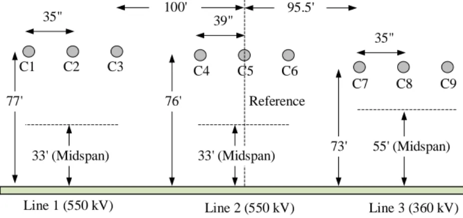
Table 2.1 Conductor data of the transmission system of Figure 2.15 ... 22

Table 2.2 Cable data for the system of Figure 2.20 ... 25

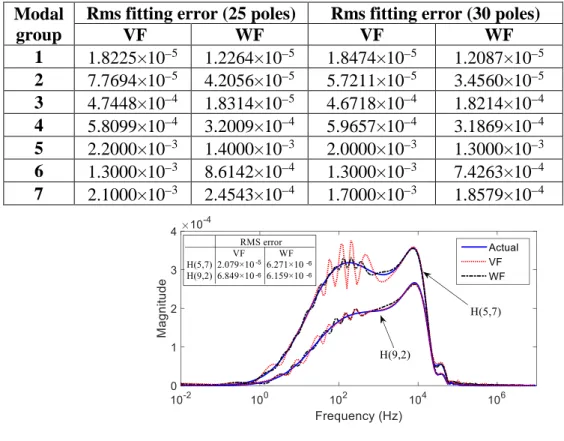
Table 3.1 Fitting errors of the modal contribution groups of the cable system of Figure 2.20 ... 34

Table 3.2 Fitting errors of the modal contribution groups of the cable system of Figure 2.20, considering the frequency partitioning approach ... 35

Table 3.3 Fitting data of the system of Figure 3.6 ... 39

Table 4.1 Residue-pole pairs with large ratios obtained with ULM ... 49

Table 4.2 Fitting errors of the modal groups of the system of Figure 4.8... 51

Table 4.3 Cable data for the system of Figure 4.18 ... 56

Table 4.4 Time-domain results (steady-state values) ... 56

Table 4.5 Steady-state magnitude results obtained by ULM ... 57

Table 5.1 Comparison of CPU times ... 67

Table 5.2 Comparison of CPU times for the simulation of Figure 5.15 ... 72

Table 6.1 Three-phase line switching, peak voltages (kV) ... 76

Table 6.2 Trapped charge voltages (kV) ... 76

Table 6.3 Source impedance data for buses along Big Eddy-Chemawa line ... 79

Table 6.4 Source voltage data for buses along Big Eddy-Chemawa line ... 79

Table 6.5 Sequence of switching times ... 80

Table 7.1 Sequence of switching events in simulation 246 ... 105

Table 7.2 Sequence of switching events in simulation 152 ... 106

Table 7.3 Summary of results ... 107

Table B.1 Suliciu model parameters ... 125

(15)

LIST OF FIGURES

Figure 2.1 Multiconductor line segment of length L ... 9

Figure 2.2 Traveling-wave multiconductor line/cable segment ... 10

Figure 2.3 Equivalent Norton circuit... 11

Figure 2.4 Classification of the currently most predominant line/cable models ... 12

Figure 2.5 Three-phase transmission line (a) physical layout, and (b) test circuit ... 18

Figure 2.6 Frequency response, (a) exact versus PI and CP and (b) exact versus FD and ULM . 18 Figure 2.7 Voltage of phase a at the receiving end, balanced energization, (a) NLT versus PI and CP and (b) NLT versus FD and ULM ... 18

Figure 2.8 Voltage of phase a at the receiving end, unbalanced energization, (a) NLT versus PI and CP and (b) NLT versus FD and ULM ... 19

Figure 2.9 25-km double-circuit transmission lines physical (a) layout and (b) test circuit ... 20

Figure 2.10 Fault current at the end of the line ... 20

Figure 2.11 Voltage at the receiving end of conductor C4 ... 20

Figure 2.12 Layout and parameters details of the 15-km cable system ... 21

Figure 2.13 Test circuit used in the example 2 ... 21

Figure 2.14 Sheath voltage of phase a at the receiving end ... 21

Figure 2.15 Three transmission lines in parallel ... 22

Figure 2.16 Network configuration for example 4 ... 23

Figure 2.17 Voltage of phase b at the receiving end of Line 2 ... 23

Figure 2.18 Voltage of phase b at the receiving end of Line 3 ... 24

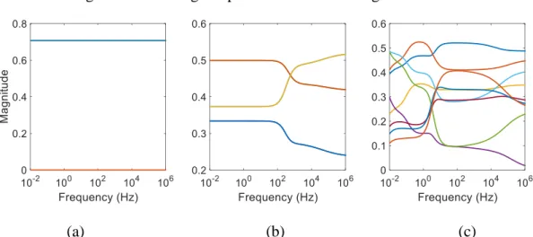
Figure 2.19 Magnitude of entries of the second column of the transformation matrix of the lines shown in: (a) Figure 2.5a, (b) Figure 2.9a and (c) Figure 2.15 ... 24

(16)

Figure 2.21 Magnitude of diagonal entries of the (a) H, and (b) Y_c matrices. ... 25

Figure 2.22 Magnitude of off-diagonal entries of the (a) H, and (b) Y_c matrices. ... 26

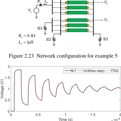
Figure 2.23 Network configuration for example 5 ... 26

Figure 2.24 Voltage at the receiving end of the first core, V₁ ... 26

Figure 2.25 Voltage at the receiving end of the fourth core, V₇ ... 27

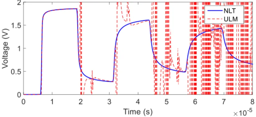
Figure 2.26 Voltage at the receiving end of the fourth core, V₁, using the ULM approach ... 27

Figure 2.27 Magnitude of (a) two diagonal and (b) two off-diagonal entries of H ... 28

Figure 3.1 Illustration of the proposed frequency partitioning method for a given entry of H ... 32

Figure 3.2 Magnitude of the H

( )

5, 7 , and H

( )

9, 2 fitted with 25 poles ... 34

Figure 3.3 Magnitude of the H

( )

5, 7 , and H

( )

9, 2 fitted with 30 poles ... 34

Figure 3.4 Magnitude of entry H

( )

5, 7 refer to Table 3.2 for rms fitting errors ... 35

Figure 3.5 Illustration of the FDM/DC approach for one entry of H ... 38

Figure 3.6 AC/DC lines geometry... 39

Figure 3.7 Low-frequency approximation of function error for H_LF ... 39

Figure 3.8 Magnitude of the first column of H. Solid line corresponds to actual values while dashed lines corresponds to fitted values with FDM/DC ... 39

Figure 4.1 Single-step integration scheme ... 44

Figure 4.2 Two-step integration scheme ... 45

Figure 4.3 Case study 1, 12-conductor cable system ... 47

Figure 4.4 Voltage at the receiving end, V₁ in Figure 4.3 ... 48

Figure 4.5 Induced voltage at the receiving end, V₇ in Figure 4.3 ... 48

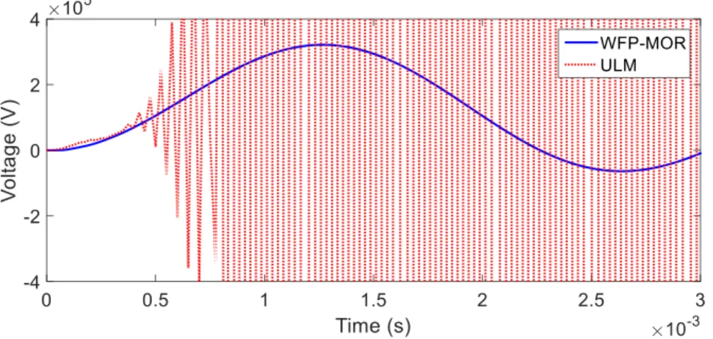
Figure 4.6 Comparison of the proposed WFP-MOR and ULM approaches ... 49

(17)

Figure 4.8 10-km transmission system layout for the case study 2 ... 50

Figure 4.9 Test circuit for the case study 2 ... 51

Figure 4.10 Sheath voltage on phase-a at the receiving end of the cable in Figure 4.9 ... 52

Figure 4.11 Induced-voltage on phase-a at the receiving end of the line in Figure 4.9 ... 52

Figure 4.12 Core-voltage of phase-a at the receiving end of the cable in Figure 4.9 ... 52

Figure 4.13 (a) short- and (b) open-circuit configuration for testing the AC/DC line ... 53

Figure 4.14 Time domain results of V₂ in Figure 4.13(a) ... 54

Figure 4.15 Time domain results of V₄ in Figure 4.13(b) ... 54

Figure 4.16 HVDC test system used for the case study 4 ... 55

Figure 4.17 Layout of the line segments in Figure 4.16 ... 55

Figure 4.18 Layout of the cable segment in Figure 4.16 ... 55

Figure 4.19 Circuit configuration of the case study 4 ... 56

Figure 4.20 Time domain results for I₄ in Figure 4.19 with time-step of 10 µs. ... 57

Figure 4.21 Hybrid AC/DC line geometry for the case study 5 ... 58

Figure 4.22 Voltage at the receiving end of C5 in Figure 4.21, time-step 10 µs ... 58

Figure 4.23 Voltage at the receiving end of C5 in Figure 4.21, time-step 10 µs ... 58

Figure 5.1 Transition steps in the proposed adaptive line model ... 61

Figure 5.2 Proposed switching control algorithm ... 62

Figure 5.3 Equivalent PI model ... 62

Figure 5.4 Tracking the steady state waveform ... 65

Figure 5.5 Finding the steady state phasor solution ... 65

Figure 5.6 Voltage of phase A at the receiving end. Simulation time of 0.16 s ... 66

Figure 5.7 Voltage of phase A at the receiving end. Simulation time of 0.5 s ... 67

(18)

Figure 5.9 Voltage of the three phases at the receiving end obtained with WB-CP model,

transient state ... 68

Figure 5.10 Voltage of phase B at the receiving end. Comparison between WB-CP and WB .... 68

Figure 5.11 Element H

( )

1,1 of the line of Figure 5.7 fitted from 0.01 Hz to 100 Hz ... 70

( )

1,1 of the line of Figure 5.7 fitted from 0.01 Hz to 100 kHz ... 70

Figure 5.13 Steady-state simulation of phase A, H fitted from 0.01 Hz to 100 kHz ... 70

( )

1,1 of the line of Figure 5.7 fitted with the FDBR technique ... 71

Figure 5.15 Voltage of phase A at the receiving end. Comparison between different models ... 71

Figure 6.1 Big Eddy-Chemawa 230-kV detailed system model [64] ... 75

Figure 6.2 One-line diagram of Big Eddy-Chemawa and parallel lines, [89] ... 77

Figure 6.3 Equivalent model for filters and capacitor banks ... 78

Figure 6.4 Simplified source model ... 78

Figure 6.5 Voltage of phase A at Chemawa end, tabulated source model ... 81

Figure 6.6 Voltage of phase A at Chemawa end, simplified source model ... 82

Figure 6.7 Voltage of phase A at the Chemawa end, comparison between tabulated and simplified source model with the FD model. ... 82

Figure 6.8 Voltage of phase A at Chemawa end, effect of the parallel lines ... 83

Figure 6.9 Voltage of phase A at the Chemawa end, effect of model refinements ... 84

Figure 6.10 Voltage of phase A at the Chemawa end considering a detailed source model ... 84

Figure 6.11 Suliciu corona model (shunt branch) with FD model for each section ... 86

Figure 6.12 Voltage of phase A at the Chemawa end with the Suliciu corona model ... 86

Figure 6.13 Voltage of phase A at Chemawa end. Comparison of Sulicio and linear corona model ... 87

Figure 6.14 Voltage of phase A at the Chemawa end. Comparison of the Suliciu and Linear Corona models. 12ms (high resolution field data). ... 87

(19)

Figure 6.15 Voltage of phase A at the Chemawa end including the Suliciu corona model for a

100-ms simulation time ... 88

Figure 6.16 Voltage of phase A at the Chemawa end. Case 5-02 ... 89

Figure 6.17 Voltage of phase A at the Chemawa end. Case 5-05 ... 89

Figure 6.18 Voltage of phase C at the Big Eddy end, Case 5-53 ... 89

Figure 6.19 Voltage of phase B at the Chemawa end, Case 1-04 ... 90

Figure 7.1 Big Eddy breaker dielectric slopes based on prestrike data during closing ... 94

Figure 7.2 Prestrike modeling in EMTP ... 94

Figure 7.3 Big Eddy breaker dielectric slope of phase A ... 95

Figure 7.4 Voltages at Big Eddy end ... 96

Figure 7.5 Voltages at Chemawa end ... 96

Figure 7.6 Voltage of phase A at Chemawa end ... 96

Figure 7.7 Systematic switching times ... 97

Figure 7.8 Maximum overvoltages from 360 simulations ... 97

Figure 7.9 Minimum overvoltages from 360 simulations ... 98

Figure 7.10 Voltages at Chemawa end, simulation 5 ... 98

Figure 7.11 Voltage of phase A at Chemawa end, simulation 5 ... 98

Figure 7.12 Gaussian distribution ... 99

Figure 7.13 Cumulative distribution function ... 99

Figure 7.14 Maximum overvoltages from 300 simulations ... 100

Figure 7.17 Maximum values obtained in Figure 7.14 ... 101

Figure 7.18 Histogram of Figure 7.17 ... 101

(20)

Figure 7.21 Minimum overvoltages values from 300 simulations ... 102

Figure 7.23 Voltage of phase C at Chemawa end, simulation 32 ... 103

Figure 7.24 Prestrike model with random times ... 103

Figure 7.25 Cumulative distribution function ... 104

Figure 7.26 Comparison of the statistical and real switching times of phase B ... 104

Figure 7.27 Maximum overvoltages values from 300 simulations ... 104

Figure 7.28 Maximum values obtained in Figure 7.27 ... 105

Figure 7.31 Minimum overvoltages values from 300 simulations ... 106

Figure 7.33 Voltage of phase C at Chemawa end, simulation 152 ... 107

Figure A.1 Inclusion of losses in the CP line model ... 122

Figure A.2 CP equivalent circuit ... 123

(21)

LIST OF SYMBOLS AND ABBREVIATIONS

AC Alternating current

BPA Bonneville Power Administration BR Balanced realization

CP Constant Parameter

DC Direct current

EMT Electromagnetic transients

EMTP Electromagnetic Transients Program

FD Frequency dependent

FDBR Frequency-domain balance realization

FDCM Frequency-dependent cable model in phase domain FDM Frequency dependent model

FDM/DC FDM with DC correction

FDQ Frequency-dependent cable model based on modal domain FFT Fast Fourier transform

H Propagation function matrix

HF High frequency

HVDC High voltage direct current

IEEE Institute of Electrical and Electronic Engineering

LF Low frequency

MPM Matrix pencil method MOR Model order reduction NLT Numerical Laplace transform

(22)

PI Lumped PI circuit

Q Transformation matrix

g

 Ground resistivity

r Radius of a conductor

R Per unit length series resistance matrix RC Parallel resistive-capacitive lumped circuit

dc

R Resistance of DC

RWB Reduced-order WB

s Complex frequency

 Propagation time delay

T Matrix of eigenvectors of the product YZ

ULM Universal line model

VF Vector fitting

WB Wideband

WB-CP Adaptive line model: switching between WB and CP WB-PI Adaptive line model: switching between WB and PI WB-RWB Adaptive line model: switching between WB and RWB WF Weighting fitting technique

WFP WF technique combined with frequency partitioning WFP-MOR WFP technique combined with MOR

Y Per unit length shunt admittance matrix

c

Y Characteristic admittance matrix

(23)

LIST OF APPENDICES

Appendix A Constant parameter line model details ... 122 Appendix B Corona model details ... 124

(24)

CHAPTER 1 INTRODUCTION

1.1 Motivation

The transmission line is one of the most important devices in the electrical power system, its primary function is to transfer electrical power from generating stations to consumers. Typically, aerial lines are used for long distances in rural zones, while underground cables are used in urban areas.

The design and effective operation of transmission lines strongly depends on accurate electromagnetic transients (EMT) simulations, which are obtained using precise line models. Line modeling is much easier when the line equations are formulated directly in the frequency domain [1], [2]. However, for transient analysis of large systems, the step-by-step time-domain solution [3] is more flexible than frequency-domain formulations, especially with the presence of nonlinear elements and switching events in the network. Thus, time-domain based models are preferred and widely used in practice.

Transmission lines are characterized by two electrical parameters, i.e., series impedance Z

(longitudinal field effects), and shunt admittance Y (transversal field effects) matrices. Considering the nature of these parameters, time-domain line models can be divided into two groups: lumped- and distributed-parameters models. In the lumped-parameter models, both Z

and Y are calculated at a single frequency. These models, also called PI models, are adequate for steady-state studies when calculating parameters at fundamental power frequency. For transient studies, the most appropriate models are those that consider line parameters distributed along the distance. These models are formulated based on the traveling-wave theory [3]-[5], and can be classified into two categories: a) constant parameters and b) frequency-dependent parameters models.

The constant parameter (CP) model considers that Z and Y are independent of the frequency effects caused by the skin effect on phase conductors and on the ground [5]. The CP model implementation requires a small computational burden [5]. However, since a transient typically involves a wide range of frequencies, the CP model is only recommended for modeling lines located on zones distant to the area where the transient event occurs.

(25)

The implementation of frequency-dependent models requires rational function-based approximations of two coefficients: the characteristic admittance Y_c, which relates current waves to voltage waves, and the propagation function H, which defines the delay and distortion of a wave traveling along the line. Rational functions allow efficient computation of convolution integrals in the time-domain through recursive schemes.

Early attempts to include frequency dependence in traveling-waves based models for transient simulations relied on performing direct numerical convolutions [6]-[8]. The major drawbacks encountered in those convolution methods are the excessive computation time and large accumulation errors. These problems were first addressed with the introduction of the recursive convolution scheme [9]-[11]. Afterwards, several models have been developed during the last decades, which can be classified into two groups: a) modal-domain, and b) phase-domain based models.

Modal-domain models

Modal-domain based models typically assume a constant transformation matrix [6]-[13]. In general, these models provide accurate representations for a large class of lines. However, when the frequency dependence of modal transformation matrices is very strong, the assumption of constant transformation matrices causes inaccuracies [14]. Therefore, their accuracy is restricted to aerial lines with symmetric or nearly-symmetric configurations.

The consideration of the frequency-dependent modal transformation can be achieved by applying a convolution to the matrix columns, as proposed in [14]. However, it has been encountered that transformation matrices cannot be synthesized with sufficient accuracy in many cases, yielding to imprecisions and numerical instabilities in time-domain simulations [15].

Phase-domain models

The issues associated with the constant transformation matrices mentioned above can be avoided by fitting the line functions directly in the phase domain [16]-[27]. However, this conveys complexities because the elements of H contain modal contributions with multiple time delays. Some models suggest extracting a single time-delay from each entry of H [18], [19]. However, this may stiffen the fitting procedure, requiring a high order fitting. This problem is addressed in other models by including modal time delays in the phase-domain formulation [21]-[27].

(26)

One of the most accepted phase-domain models is the universal line model (ULM) [27], which has been implemented in many EMTP-type programs. The ULM has a two-step fitting approach in which the poles of H are identified in the modal domain together with time delays, and the residues in the phase domain. Repetitive or close modal delays are grouped. The criterion for grouping is the difference in angle and magnitude at a high frequency [28]-[30]. Since its proposal, ULM has received several improvements related to fitting accuracy [31], out-of-band passivity violations [32]-[33], matrix symmetry issues [34], and real-time implementation [35]. Although the ULM is considered an accurate model for both transmission lines and cables, it has been associated with numerical stability problems [36]-[39]. These problems potentially arise when the propagation function H is fitted with poles and delays coming from different but close delay groups. This is denoted as unbalanced modal contributions and it results in magnification of integration errors in time-domain simulations. Adapting more accurate integration methods and a two-step interpolation scheme, as proposed in [37], reduces integration errors and helps maintaining numerical stability in the time domain. However, the unbalanced modal contributions in H cannot be removed by changing the integration method, and inaccurate simulation results with spurious oscillations can still be observed in cases with high residue/pole ratios.

Fitting modal contribution groups of H directly in the phase-domain, as proposed in [39], avoids high residue/pole ratios. However, if the fitting of H is performed directly in the phase domain and per modal contribution, more poles are required compared to ULM approach to maintain similar precisions. Moreover, since a single set of poles is used per modal contribution group to accelerate time domain simulations, the overall system of equations becomes large, and off-diagonal low-magnitude entries of H may not be accurately fitted. Even though off-diagonal entries of H are of very small magnitude, their poor fitting may have an observable impact on induced transient voltages.

Curve fitting techniques

The basic idea of frequency-dependent line models in EMT-type programs is to use rational approximations for Y_c and H, calculated by using different methodologies. Among existing methodologies, the vector fitting (VF) method has been widely used for the fitting of measured or calculated frequency-domain functions with rational function approximations [40]. Alternatively,

(27)

the matrix pencil method (MPM) [46] has also been applied to rational fitting of frequency responses [47], [48]. However, the MPM is not as direct as VF method, since it requires additional numerical operations from and to the time-domain and the frequency-domain, involving a set of closed-form formulas based on the Fourier transform [49].

After its original proposal, the VF method has been modified to improve its numerical performance [41]-[43]. However, its equations may become ill-conditioned for wide frequency ranges, creating problems for low order rational fitting. To address this problem, the orthonormal vector fitting, and the weighted vector fitting have been proposed in [44], and [45], respectively. Partitioning of frequency responses improves fitting precision. This idea has been applied for the modeling of frequency dependent network equivalents [50]-[52], transmission lines [53], and underground cables [54]. The downside is the increasing number of poles. Recently, the application of a model order reduction [52] via a balance-realization (BR)-based technique [55], [56] has been proposed to remove the redundant poles.

Corona effect

It has been mentioned the importance of including the frequency dependence of line parameters in the line modeling. However, even though frequency dependent line models provide accurate time-domain simulations, conservative results can be obtained unless the corona effect is considered [57]. The corona effect has a strong influence on the propagation of waves [57]-[63]. The corona discharge is produced by the ionization of the air surrounding a conductor that is electrically charged. This occurs when the voltage of a conductor reaches a critical value, i.e. corona inception voltage [59]. The storage and movement of charges in the ionized region can be viewed as an increase of the conductor radius and consequently of the capacitance to ground [58]. The effect of corona is characterized by the charge-voltage (q-v) response of the conductors of the transmission line [59].

The representation of corona involves a distributed nonlinear hysteresis behavior which becomes difficult to combine with the EMTP-type transmission line formulations. Most of the methods proposed in the literature rely on the two following techniques: i) subdividing lines in linear subsections with non-linear shunt branches at each junction [58], and ii) applying finite differences methods to line equations [60]. The latter presents less numerical oscillations than the former; however, it requires a significant computational burden [60].

(28)

Existing corona models can be classified into two groups: static and dynamic. In general, all the models need to calculate beforehand the corona inception voltage [59]. Static models are those in which the corona capacitance is only a function of the voltage. In this type of models, a fixed nonlinear q-v characteristic is assumed, and can be either simulated directly by using RC circuits and diodes [61], or described by analytical expressions [62]. Dynamic models consider the fact that the charge depends on the voltage and on the rate of change of the voltage [63].

1.2 Contributions

EMT simulations require covering a wide range of frequencies including those very close to DC. As mentioned before, several line and cable models have been developed during the last decades [3]-[27]. It is concluded that the more sophisticated models suffer from computational performance issues, and the simplified models are not sufficiently accurate when they are used in a wide range of transients.

This thesis first reviews the most predominant models in the literature and demonstrates their drawbacks through simulations. Then, it investigates the modeling practice required to obtain more accurate and faster time-domain simulations using frequency-dependent line/cable models. The contributions of this thesis are detailed as follows.

A) Identification procedure of the propagation function

This thesis contributes with precise fitting procedures for the identification of H in the phase domain while maintaining reduced order of approximation. In the proposed fitting approach, poles and residues of H are identified simultaneously in the phase domain. The procedure encapsulates the following proposed features. An adaptive weighting technique is applied to normalize all the entries of H prior to fitting. This allows ensuring the precision of fitting for all the entries including the low-magnitude off-diagonal elements. The frequency band of fitting is partitioned so that the fitting problem is simplified, and the accuracy is improved compared to the standard application of vector fitting. Finally, a model order reduction (MOR) technique via balanced realization (BR) is applied to obtain a reduced order of approximation.

The proposed methodology allows obtaining more accurate fitting, and when combined with more precise integration schemes, it yields more stable and more accurate time-domain simulations.

(29)

B) DC correction in wideband models

Transient analysis of transmission lines with accurate capturing of the DC response, has become of special interest with the increasing number of planned and installed HVDC systems [65]-[68]. One practice to capture the DC response in the ULM is to specify a very low frequency for fitting

H and Y_c. However, this approach often leads to incorrect solutions for the DC steady-state voltages and currents due to generally poor DC fitting [69]-[70]. To address this problem, this thesis contributes with a two-stage fitting method in which low frequency samples are given priority. In the first stage, the fitting is performed by excluding very low frequency samples such as those below 1 Hz. In the second stage, a correction function is found for the excluded low frequency samples. It is proposed to use this approach for avoiding numerical instabilities due to unbalanced fitting, and for improving the precision of DC response.

C) Adaptive line modeling

Another contribution of this thesis is a relaxation method that can monitor the frequency content of a transient and adjust model mathematics accordingly to achieve better performance without significant loss of accuracy. Simulation of EMT using relaxing models have been proposed through the shift frequency concept [71]-[74]. In this thesis, it is proposed to switch between wideband (WB) and PI models during the simulation. Basically, the idea is to relax the line equations during the steady state to increase the speed of the EMT-type computations. The switching between the two models is performed by modifying the terms of the history current vectors and their corresponding elements in the nodal admittance matrix during the simulation.

D) Validation of line models with field measurements

One more contribution of this thesis is to validate transmission lines model with field tests and to identify the required simulation practices in reproducing field measured overvoltages in EMT simulations. The test data are available through an IEEE working group from Bonneville Power Administration (BPA). It is demonstrated that even though the pattern of the transient voltage waveforms can be reproduced very well using frequency-dependent line models, simulations results are significantly overestimated unless the effect of corona is included. Two types of corona models are tested; both models demonstrate that corona is the primary factor that allows the simulations to correctly reproduce field measurements.

(30)

E) Statistical study of switching overvoltages

This thesis also contributes with an investigation on statistical simulations of switching overvoltages to determine the worst overvoltage at the receiving end of a transmission line with trapped charge.

1.3 Thesis outline

This thesis is composed of eight chapters and two appendices.

CHAPTER 1 – INTRODUCTION, explains the background motivating this PhD project, and summarizes its objectives and contributions.

CHAPTER 2 – REVIEW OF LINE/CABLE MODELS, contains the basic theory essential for a better understanding of the content of this thesis. This includes main equations and a general classification of line and cable models. In addition, it demonstrates the drawback of current models through time-domain simulations.

CHAPTER 3 – ENHANCED FITTING TECHNIQUES FOR THE IDENTIFICATION OF THE PROPAGATION FUNCTION, presents fitting procedures for the identification of the propagation function in the phase domain. The proposed procedure encapsulates: Frequency partition and adaptive weighting techniques to ensure the precision of fitting, and a model order reduction method via balanced realization to obtain a reduced order of approximation. It also includes an additional two-stage fitting procedure for improving the precision of DC response. CHAPTER 4 – TIME DOMAIN SIMULATIONS, analyses the impact of improving the fitting of the propagation function in time-domain simulations via transient studies. The proposed fitting procedures are combined with more precise integration schemes to obtain stable and more accurate simulation results.

CHAPTER 5 – ADAPTIVE LINE MODEL, presents a relaxation method to increase the speed of time-domain simulations. It is proposed to switch between WB and PI models during the simulation. The idea is illustrated via a simple case of study.

CHAPTER 6 – SIMULATION OF SWITCHING OVERVOLTAGES AND VALIDATION WITH FIELD TEST, presents the analysis of other important factors in line modeling, such the consideration of corona. It includes validation of transmission lines with field test.

(31)

CHAPTER 7 – STATISTICAL SIMULATIONS OF SWITCHING OVERVOLTAGES, presents a statistical simulation study to determine the worst overvoltage at the receiving end of a transmission line during high-speed reclosing with a trapped charge on the line.

CHAPTER 8 – CONCLUSION, presents the main conclusions of this thesis, the list of publications derived from its contributions and possible future work.

APPENDIX A – CONSTANT PARAMETER LINE MODEL DETAILS, presents the time-domain implementation details of the constant parameter line model.

APPENDIX B – CORONA MODEL DETAILS, summarizes the equations and parameters of the corona models used in Chapter 6.

(32)

CHAPTER 2 REVIEW OF LINE/CABLE MODELS

This chapter presents the basic theory related to line/cable modeling, including main equations and a general classification of time-domain models. In addition, it demonstrates the drawback of current models used for EMT through time-domain simulations.

2.1 Main equations

2.1.1 Equations in the frequency domain

Most of existing transmission line models for EMT simulations are based on the traveling-wave theory [3]. Figure 2.1 illustrates reference directions of a transmission line of length L assuming

N conductors parallel to the ground.

L I L V 0 I 0 V N 2 1 0 x = x=L

Figure 2.1 Multiconductor line segment of length L

At each point of the line depicted in Figure 2.1, the frequency domain line equations are expressed as: d dx = − V ZI (2.1) d dx= − I YV (2.2)

where Z and Y are the per unit length series impedance (longitudinal field effects) and shunt admittance (transversal field effects) matrices, respectively. Both Z and Y can be numerically obtained from the geometry and the electrical parameters of the line [75].

The general solution of (2.1) and (2.2) can be expressed as [4]:

( )

x x x =e−Γ _F+eΓ _B I I I (2.3)

( )

1

(

x x

)

x = _c− e−Γ _F−eΓ _B V Y I I (2.4)

(33)

where Γ= YZ; the forward and backward currents, I_F and I_B, can be obtained from the boundary conditions of the line. The characteristic admittance matrix Y_c is given by:

1 − =

c

Y ΓZ (2.5)

In EMTP-type models, the transmission line/cable is represented by decomposing the current waves into incident and reflected waves as depicted in Figure 2.2.

k V V_m k I Im c H, Y ki I kr I mi I mr I k m

Figure 2.2 Traveling-wave multiconductor line/cable segment

Based on (2.3) and (2.4), and the reference directions given in Figure 2.2, the frequency-domain voltages and currents at both ends are related by:

(

)

= − + = − k k c k m c m sh ki I Y V H I Y V I I (2.6)

(

)

= − + = − m m c m k c k sh mi I Y V H I Y V I I (2.7)

where I_k and I_m are the vectors of injected currents, and V_k and V_m correspond to nodal voltage vectors. Also, subscripts i and r refer to incident and reflected waves, respectively. H is the propagation function matrix defined by:

L e−

= Γ

H (2.8)

Equivalently, the model defined by (2.6) and (2.7) can be expressed in terms of a two-port network. Combining (2.6) and (2.7), and defining U as the identity matrix, the two-port model is given by:

(

)

2 1 2 2 2 2 −   + −    ₌ ₋           − +        k k c m m I H U H V U H Y I _H _H _U V (2.9)

(34)

2.1.2 Equations in the time domain

To obtain the time-domain counterparts of (2.6) and (2.7), convolution operations (denoted by ) at line/cable terminals must be performed, as indicated in (2.10) to (2.13) (time-domain variables indicated with lowercase letters).

=  k sh c k i y v (2.10) =  m sh c m i y v (2.11)

(

)

=  + =  m ki m sh mr i h i i h i (2.12)

(

)

=  + =  k mi k sh kr i h i i h i (2.13)

The objective is to obtain the Norton equivalent shown in Figure 2.3 by solving the time-domain versions of (2.6) and (2.7). The history current sources in Figure 2.3 are obtained using the convolutions involved in (2.10) to (2.13). The

c

Y

G term is calculated from the convolution of the characteristic admittance with a terminal voltage.

k i vk vm im k hist i m hist i c Y G c Y G

Figure 2.3 Equivalent Norton circuit

The time-domain implementation of this type of model requires the synthesis of H and Y_c. The identification of rational functions for these two matrices is not straightforward, particularly in the case of H due to multiple time delays [27].

2.2 Classification of line/cable models

Figure 2.4 presents a general classification of the most commonly used transmission line/cable models for EMT simulations. Considering the nature of Z and Y, the line models can be divided into two groups: 1) lumped- and 2) distributed-parameters models.

(35)

Line/cable models

Lumped parameters Distributed parameters

Constant parameters

Frequency-dependent parameters PI model

CP model Modal domain Phase domain

FD model FDQ model

Universal line model (ULM)

Frequency-dependent cable model (FDCM)

Figure 2.4 Classification of the currently most predominant line/cable models

2.2.1 Lumped parameter models

In the lumped parameter models, or PI models, the coefficients Z and Y are calculated at a single frequency; thus, (2.9) can be directly used for modeling a line segment. For a time-domain simulation, the model of (2.9) can be discretized according to the integration time-step and solved at each simulation time-point [4]. However, since this model is only capable to simulate one frequency, its application is only adequate for steady-state purposes. For instance, harmonic initialization and frequency scan solutions.

2.2.2 Distributed parameter models

For EMT simulations, the most appropriate models are those that consider the parameters distributed along the distance. These models use (2.6) and (2.7) to represent the line at each end by a Norton equivalent circuit [4], as shown in Figure 2.3. This group of models may consider the parameters Z and Y as: a) constant- or, b) frequency-dependent.

The constant parameter (CP) model considers that (2.6) and (2.7) are resolved independently of the frequency effects, avoiding numerical convolution operations and consequently requiring a small computational burden [5]. However, since the propagation modes cannot be represented at high frequencies, the CP model is only recommended for modeling lines in analysis of problems with limited frequency dispersion.

(36)

The basic idea of frequency-dependent line models in EMT-type programs is to use rational approximations for Y_c and H, calculated by using different methodologies [40]-[46]. Rational functions allow efficient computation of convolution integrals through recursive schemes. The identification of Y_c and H is not straightforward, particularly in the case of H, due to multiple time delays [30]. Several frequency-dependent line models have been proposed during the last decades [6]-[27], the most predominant ones are reviewed in the next section.

2.3 Frequency-dependent models

Frequency-dependent line and cable models used for EMT simulations can be divided into two groups: a) modal-domain, and b) phase-domain based models.

2.3.1 FD model (modal domain)

In the frequency-dependent line model proposed in [12], named in this thesis as FD model, the multiphase line functions are decoupled via modal transformation. The transformation matrix used to relate modal and phase quantities is assumed to be constant and real. The line functions, i.e., the characteristic impedance Z_c and the propagation function H, in the modal domain are calculated as: m ₌ T c c Z Q Z Q (2.14) m ₌ −1 H Q HQ (2.15)

where Q is the eigenvector matrix which diagonalizes the product YZ and superscript m indicates modal quantity. The FD model represents frequency dependence by fitting Z_c and H

for each mode using a Bode approximation [12]. Then, each mode is solved separately as a single-phase circuit. For time-domain implementation details see [12].

Synthesis of the characteristic impedance

In the fitting procedure presented in [12], the characteristic impedance Z_c is formulated by a series of RC parallel blocks. The rational function of each mode m of Z is of the form m_c

(37)

(

)(

) (

)

(

11

)(

22

) (

)

M m c M s z s z s z Z K s p s p s p + + + = + + + (2.16)

where z_i and p_i are real and positive zeros and poles, respectively, and K is a constant value. Equivalently, (2.16) can be expressed as a partial fraction expansion as follows

0 1 M m i c i i k Z k s p = = + +



(2.17)

where M is the order of approximation, k₀ is a constant value, and k_i and p_i represents its ith pole and its ith residue, respectively.

Synthesis of the propagation function

The modes of the propagation function H are normalized as minimum-phase-shift functions prior to fitting [12]. The propagation modes are represented by the rational approximation of the form ( ) 1 m M s m i i i k H e s p  − =  −



(2.18)

where  is a real constant value associated with a modal time delay.

Frequency-dependent transformation matrix

The FD model provides accurate representations for a large class of line configurations. However, their accuracy is restricted to cases where the frequency dependence of the transformation matrix Q is not very strong, i.e., aerial lines with symmetric or nearly symmetric configuration; thus, it is not applicable to cables.

The consideration of the frequency-dependent modal transformation in the model can be achieved by applying additional convolution operations to the transformation matrix elements, as proposed in the cable model presented in [14]. In this model, named in this thesis as FDQ model, each entry of the full transformation matrix Q is approximated with

0 1 M i i i k Q k s p = = + +



(2.19)

(38)

To obtain the rational approximation of the entries of Q, its eigenvectors are normalized prior to fitting, so that one of its elements becomes real and constant along the entire frequency range. This procedure allows that all the entries of Q become minimum-phase-shift functions. It is noted that Q can be fitted only when its elements are continuous function of frequency [14].

2.3.2 ULM (phase domain)

The ULM [27] accounts for frequency-dependent parameters and constitutes a wideband model. Although ULM has its bases on modal factorization, it resolves the multiconductor propagation relations in the phase domain. Thus, it provides highly accurate results for the simulation of coupling effects between parallel conductors, compared to the modal-domain based models.

Fitting of the characteristic admittance

The fitting of the characteristic admittance Y_c is not stringent as it exhibits smooth behavior in the frequency-domain. The following form is used [27]:

1 y N i i i= s q  + −



c 0 G Y G (2.20)

where N_y is the order of approximation, q_i represents the ith fitting pole, G_i is the matrix of residues, and G₀ is a constant matrix representing the limit of Y_c when s → .

Fitting of the propagation function

In ULM, H is first decoupled into single-delay terms through modal decomposition m −1

=

H TH T (2.21)

where T is the matrix of eigenvectors of the product YZ, and Hm is a matrix of the form

(

1 2

)

m , , , N diag e e e = H (2.22)

where the terms _ei_{are the eigenvalues of} _H_{, representing the propagation modes}

i H . To compensate excessive phase lag and achieve a low-order rational approximation, a constant time delay is removed prior to fitting. Therefore, poles and delays are identified by fitting each modal propagation function with

(39)

( ) , 1 i i M j s i i j j c H e s p  − =  −



(2.23)

where M_i is the order of the approximation for the ith mode, p_{i j}_, represents the jth pole, c_j

represents its jth residue, and  is the time associated to the ith mode. Repetitive or close modal _i delays are grouped. The criterion for grouping is the difference in angle and magnitude at a high frequency [27]. Once the poles and delays are known, the matrix of residues is found by solving the following overdetermined problem:

( ) , , 1 1 gr _i i N _M i j s i j i j e s p  − = =    _ _ −  

 

R H (2.24)

where N_gr is the number of modal groups, and R_{i j}_, corresponds to the matrix of residues.

2.3.3 FDCM (phase domain)

Although (2.24) can be used for any cable or line configuration, it has been associated with numerical stability problems due to the existence of residue pole pairs with high ratios and opposite signs coming from different but close delay groups [39]. This results in a magnification of integration and interpolation errors in time-domain simulations.

In the frequency-dependent cable model (FDCM) proposed in [39], H is decomposed into modal contributions groups which are individually fitted in the phase domain. In FDCM, similar eigenvalues of H and their corresponding eigenvectors are grouped by summing them, and a single time delay is assigned to the group. The resulting modal contribution groups are smooth functions of frequency [39]. Thus, H in (2.24) is expressed now with:

1 ˆ gr i N s i i e− = 



H H (2.25)

where N is the number of modal contribution groups ˆ_gr H . The fitting of _i H is directly performed on each modal contribution group to obtain poles and residues simultaneously; consequently, the high residue/pole ratios encountered in ULM are eliminated. In (2.25), a

(40)

common set of poles can be used for each modal contribution. The exponential time delay  _i term is removed prior to fitting, i.e.

, , 1 ˆ Mi i j i i j j= s p  −



R H (2.26)

The fitting of Y_c in FDCM is performed using (2.20) due to its smooth behavior in the frequency domain.

2.4 Discussion on line and cable models

This section aims to evaluate and to discuss the performance of the most predominant line and cable models used for EMT analysis. The drawbacks of such models are demonstrated trough transient simulation of practical cases. The models and routines currently implemented in EMTP are adopted for the time-domain simulations. For verification purposes, the simulation results obtained with the numerical Laplace transform (NLT) technique [2], are considered as reference solution.

2.4.1 Importance of frequency dependence of line parameters

The objective of this section is to show that frequency-dependent models are required to achieve accurate results in EMT studies.

2.4.1.1 Example 1: Energization of an overhead transmission line

This example considers the three-phase transmission line system of Figure 2.5. Figure 2.6 shows the frequency response of the Thevenin impedance seen from the source side (see Figure 2.5b), when the transmission line is represented with the line models of Figure 2.4. It can be observed that the PI model is able to represent only one resonant frequency, while the CP model loses precision at high frequencies. On the contrary, the frequency-dependent models, i.e., FD and ULM, are able to provide accurate results for the entire frequency range, compared to the exact solution obtained with (2.9).

For time-domain analysis, the line of Figure 2.5a is modeled with the approaches of Figure 2.4 and energized by a three-phase voltage source of 230 kV, see Figure 2.5b. Figure 2.7 shows the voltage of phase a at the receiving end of the line when the three phases are simultaneously

(41)

closed at t =_c 0 s. It is observed that FD and ULM provide accurate results when compared to NLT, while both CP and PI models are not able to properly reproduce the high frequency dispersion of the transient. This phenomenon is more evident in an unbalanced energization. Figure 2.8 shows the time-domain results when the closing times t_c are 1 ms, 6 ms, and 4 ms, for the phases a, b, and c, respectively.

ρg = 100 -m 20 m 10 m Phase wires: Rdc = 0.0701 /km r = 1.529 cm 14 m 9 m Ground wires: Rdc = 3.75 /km r = 0.475 cm tc 193.1 km 0 V V_L a b c s V (a) (b)

Figure 2.5 Three-phase transmission line (a) physical layout, and (b) test circuit

(a) (b)

Figure 2.6 Frequency response, (a) exact versus PI and CP and (b) exact versus FD and ULM

(a) (b)

Figure 2.7 Voltage of phase a at the receiving end, balanced energization, (a) NLT versus PI and CP and (b) NLT versus FD and ULM

(42)

(a) (b)

Figure 2.8 Voltage of phase a at the receiving end, unbalanced energization, (a) NLT versus PI and CP and (b) NLT versus FD and ULM

2.4.1.2 Example 2: Single-phase fault on a double circuit transmission line

This case study aims at analyzing the transient response of a faulted transmission line. For this analysis, the first circuit of the 231-kV double-circuit transmission line of Figure 2.9 is submitted to a single-phase fault. It is considered that the fault occurs at the receiving end of the first conductor (phase a), as shown in Figure 2.9b. The sending end of the second circuit is grounded by a resistor of 1 Ω while the receiving end is left open.

Figure 2.10 shows the transient response of the fault current when the line of Figure 2.9 is modeled with the CP, FD, and ULM. The frequency band considered in the fitting of line function in both FD and ULM is from 0.01 Hz to 1 MHz. As for the CP, the line parameters are calculated at 1 kHz. The simulation time-step is of 10 μs for all models. It is observed in Figure 2.10 that frequency-dependent models, i.e., FD and ULM, provide identical results, which significantly differ from the response obtained with the CP model. This is explained as follows. Although CP model considers the distributed nature of the line parameters, this model is not capable to represent the high frequency dispersion occurred during the fault. The effect of the frequency dependence is more noticeable in the transient waveform of induced voltages at the end of the line. For example, Figure 2.11 shows the induced voltage on the fourth conductor C4. Note that the minor deviation between the simulation obtained with the FD and ULM approach is attributed to the accuracy of fitting process obtained in each model. It is remarked that the FD model is based on the modal domain, while the ULM performs the fitting in the phase domain.

Accurate and Efficient Simulation of Electromagnetic Transients Using Frequency Dependant Line and Cable Models

POLYTECHNIQUE MONTRÉAL

Accurate and efficient simulation of electromagnetic transients using

frequency dependent line and cable models

POLYTECHNIQUE MONTRÉAL

Accurate and efficient simulation of electromagnetic transients using

frequency dependent line and cable models

DEDICATION

ACKNOWLEDGEMENTS

RÉSUMÉ

ABSTRACT

TABLE OF CONTENTS

LIST OF TABLES

LIST OF FIGURES

( )

( )

( )

( )

( )

( )

( )

( )

LIST OF SYMBOLS AND ABBREVIATIONS

LIST OF APPENDICES

CHAPTER 1

INTRODUCTION

1.1 Motivation

1.2 Contributions

1.3 Thesis outline

CHAPTER 2

REVIEW OF LINE/CABLE MODELS

2.1 Main equations

2.1.1 Equations in the frequency domain

( )

( )

(

)

(

)

(

)

(

)

2.1.2 Equations in the time domain

(

)

(

)

2.2 Classification of line/cable models

2.2.1 Lumped parameter models

2.2.2 Distributed parameter models

2.3 Frequency-dependent models

2.3.1 FD model (modal domain)

(

)(

) (

)

(

)(

) (

)







2.3.2 ULM (phase domain)



(

)



 

2.3.3 FDCM (phase domain)





2.4 Discussion on line and cable models

2.4.1 Importance of frequency dependence of line parameters