HAL Id: hal-01097328
https://hal-mines-paristech.archives-ouvertes.fr/hal-01097328
Submitted on 19 Dec 2014
HAL is a multi-disciplinary open access
archive for the deposit and dissemination of
sci-entific research documents, whether they are
pub-lished or not. The documents may come from
teaching and research institutions in France or
L’archive ouverte pluridisciplinaire HAL, est
destinée au dépôt et à la diffusion de documents
scientifiques de niveau recherche, publiés ou non,
émanant des établissements d’enseignement et de
recherche français ou étrangers, des laboratoires
Parallelizing with BDSC, a resource-constrained
scheduling algorithm for shared and distributed memory
systems
Dounia Khaldi, Pierre Jouvelot, Corinne Ancourt
To cite this version:
Dounia Khaldi, Pierre Jouvelot, Corinne Ancourt. Parallelizing with BDSC, a resource-constrained
scheduling algorithm for shared and distributed memory systems. Parallel Computing, Elsevier, 2015,
41, pp.66 - 89. �10.1016/j.parco.2014.11.004�. �hal-01097328�
Parallelizing with BDSC, a Resource-Constrained
Scheduling Algorithm for Shared and Distributed
Memory Systems
Dounia Khaldia,∗, Pierre Jouvelotb, Corinne Ancourtb
aDepartment of Computer Science
University of Houston, Houston, Texas
bMINES ParisTech, PSL Research University, France
Abstract
We introduce a new parallelization framework for scientific computing based on BDSC, an efficient automatic scheduling algorithm for parallel programs in the presence of resource constraints on the number of processors and their local memory size. BDSC extends Yang and Gerasoulis’s Dominant Sequence Clus-tering (DSC) algorithm; it uses sophisticated cost models and addresses both shared and distributed parallel memory architectures. We describe BDSC, its integration within the PIPS compiler infrastructure and its application to the parallelization of four well-known scientific applications: Harris, ABF, equake and IS. Our experiments suggest that BDSC’s focus on efficient resource man-agement leads to significant parallelization speedups on both shared and dis-tributed memory systems, improving upon DSC results, as shown by the com-parison of the sequential and parallelized versions of these four applications running on both OpenMP and MPI frameworks.
Keywords: Task parallelism, Static scheduling, DSC algorithm, Shared mem-ory, Distributed memmem-ory, PIPS
1. Introduction
“Anyone can build a fast CPU. The trick is to build a fast system.” At-tributed to Seymour Cray, this quote is even more pertinent when looking at multiprocessor systems that contain several fast processing units; parallel system architectures introduce subtle system constraints to achieve good performance. Real world applications, which operate on a large amount of data, must be able to deal with limitations such as memory requirements, code size and processor
∗
Corresponding author, phone: +1 (713) 743 3362 Email addresses: [email protected](Dounia Khaldi), [email protected](Pierre Jouvelot), [email protected](Corinne Ancourt)
features. These constraints must also be addressed by parallelizing compilers that target such applications and translate sequential codes into efficient parallel ones.
One key issue when attempting to parallelize sequential programs is to find solutions to graph partitioning and scheduling problems, where vertices repre-sent computational tasks and edges, data exchanges. Each vertex is labeled with an estimation of the time taken by the computation it performs; similarly, each edge is assigned a cost that reflects the amount of data that need to be exchanged between its adjacent vertices. Task scheduling is the process that assigns a set of tasks to a network of processors such that the completion time of the whole application is as small as possible while respecting the dependence constraints of each task. Usually, the number of tasks exceeds the number of processors; thus some processors are dedicated to multiple tasks. Since finding the optimal solution of a general scheduling problem is NP-complete [1], provid-ing an efficient heuristic to find a good solution is needed. Efficiency is strongly dependent here on the accuracy of the cost information encoded in the graph to be scheduled. Gathering such information is a difficult process in general, in particular in our case where tasks are automatically generated from program code.
Scheduling approaches that use static predictions of task characteristics such as execution time and communication cost can be categorized in many ways, such as static/dynamic and preemptive/non-preemptive. Dynamic (on-line) schedulers make run-time decisions regarding processor mapping whenever new tasks arrive. These schedulers are able to provide good schedules even while managing resource-constraints (see for instance Tse [2]) and are particularly well suited when task time information is not perfect, even though they introduce run-time overhead. In this class of dynamic schedulers, one can even distinguish between preemptive and non-preemptive techniques. In preemptive schedulers, the current executing task can be interrupted by an other higher-priority task, while, in a non-preemptive scheme, a task keeps its processor until termination. Preemptive scheduling algorithms are instrumental in avoiding possible dead-locks and for implementing real-time systems, where tasks must adhere to spec-ified deadlines. EDF (Earliest-Deadline-First) [3] and EDZL (Earliest Deadline Zero Laxity) [4] are examples of preemptive scheduling algorithms for real-time systems. Preemptive schedulers suffer from possible loss of predictability, when overloaded processors are unable to meet the tasks’ deadlines.
In the context of the automatic parallelization of scientific applications we focus on in this paper, for which task time can be assessed with rather good pre-cision (see Section 4.2), we decide to focus on (non-preemptive) static schedul-ing policies1. Even though the subject of static scheduling is rather mature (see Section 6.1), we believe the advent and widespread market use of multi-core ar-chitectures, with the constraints they impose, warrant to take a fresh look at its
1
Note that more expensive preemptive schedulers would be required if fairness concerns were high, which is not frequently the case in the applications we address here.
potential. Indeed, static scheduling mechanisms have, first, the strong advan-tage of reducing run-time overheads, a key factor when considering execution time and energy usage metrics. One other important advantage of these sched-ulers over dynamic ones, at least over those not equipped with detailed static task information, is that the existence of efficient schedules is ensured prior to program execution. This is usually not an issue when time performance is the only goal at stake, but much more so when memory constraints might impede a task to be executed at all on a given architecture. Finally, static schedules are predictable, which helps both at the specification (if such a requirement has been introduced by designers) and debugging levels.
We introduce thus a new non-preemptive static scheduling heuristic that strives to give as small as possible schedule lengths, i.e., parallel execution time, in order to extract the task-level parallelism possibly present in sequential pro-grams, while enforcing architecture-dependent constraints. Our approach takes into account resource constraints, i.e., the number of processors, the computa-tional cost and memory use of each task and the communication cost for each task exchange2, to provide hopefully significant speedups on realistic shared and distributed computer architectures. Our technique, called BDSC, is based on an existing best-of-breed static scheduling heuristic, namely Yang and Gera-soulis’s DSC (Dominant Sequence Clustering) list-scheduling algorithm [5] [6], that we equip to deal with new heuristics that handle resource constraints. One key advantage of DSC over other scheduling policies (see Section 6), besides its already good performance when the number of processors is unlimited, is that it has been proven optimal for fork/join graphs: this is a serious asset given our focus on the program parallelization process, since task graphs repre-senting parallel programs often use this particular graph pattern. Even though this property may be lost when constraints are taken into accounts, our exper-iments on scientific benchmarks suggest that our extension still provides good performance speedups (see Section 5).
If scheduling algorithms are key issues in sequential program parallelization, they need to be properly integrated into compilation platforms to be used in practice. These environments are in particular expected to provide the data required for scheduling purposes, a difficult problem we already mentioned. Be-side BDSC, our paper introduces also new static program analysis techniques to gather the information required to perform scheduling while ensuring that resource constraints are met, namely a static instruction and communication cost models, a data dependence graph to enforce scheduling constraints and static information regarding the volume of data exchanged between program fragments.
The main contributions of this paper, which introduces a new task-based parallelization approach that takes into account resource constraints during the
2
Note that processors are usually not considered as a resource in the literature dealing with scheduling theory. One originality of the approach used in this paper is to suggest to consider this factor as a resource among others, such as memory limitations.
static scheduling process, are:
• “Bounded DSC” (BDSC), an extension of DSC that simultaneously han-dles two resource constraints, namely a bounded amount of memory per processor and a bounded number of processors, which are key parameters when scheduling tasks on actual parallel architectures;
• a new BDSC-based hierarchical scheduling algorithm (HBDSC) that uses a new data structure, called the Sequence Data Dependence Graph (SDG), to represent partitioned parallel programs;
• an implementation of HBDSC-based parallelization in the PIPS [7] source-to-source compilation framework, using new cost models based on time complexity measures, convex polyhedral approximations of data array sizes and code instrumentation for the labeling of SDG vertices and edges; • performance measures related to the BDSC-based parallelization of four significant programs, targeting both shared and distributed memory ar-chitectures: the image and signal processing applications Harris and ABF, the SPEC2001 benchmark equake and the NAS parallel benchmark IS. This paper is organized as follows. Section 2 presents the original DSC al-gorithm that we intend to extend. We detail our alal-gorithmic extension, BDSC, in Section 3. Section 4 introduces the partitioning of a source code into a Se-quence Dependence Graph (SDG), our cost models for the labeling of this SDG and a new BDSC-based hierarchical scheduling algorithm (HBDSC). Section 5 provides the performance results of four scientific applications parallelized on the PIPS platform: Harris, ABF, equake and IS. We also assess the sensitivity of our parallelization technique on the accuracy of the static approximations of the code execution time used in task scheduling. Section 6 compares the main existing scheduling algorithms and parallelization platforms with our approach. Finally Section 7 concludes the paper and addresses future work.
2. List Scheduling: the DSC Algorithm
In this section, we introduce the notion of list-scheduling heuristics and present the list-scheduling heuristic called DSC [5].
2.1. List-Scheduling Processes
A labelled direct acyclic graph (DAG) G is defined as G = (T, E, D), where (1) T = vertices(G) is a set of n tasks (vertices) τ annotated with an estimation of their execution time task time(τ ), (2) E, a set of m edges e = (τi, τj) between two tasks, and (3) D, a n × n communication edge cost matrix edge cost(e); task time(τ ) and edge cost(e) are assumed to be numeri-cal constants, although we show how we lift this restriction in Section 4.2. The functions successors(τ, G) and predecessors(τ, G) return the list of immediate successors and predecessors of a task τ in the DAG G. Figure 1 provides an
entry 0 τ1 1 τ4 2 τ2 3 τ3 2 exit 0 0 0 2 1 1 0 0
step task tlevel blevel DS scheduled tlevel
κ0 κ1 κ2
1 τ4 0 7 7 0*
2 τ3 3 2 5 2 3*
3 τ1 0 5 5 0*
4 τ2 4 3 7 2* 4
Figure 1: A Directed Acyclic Graph (left) and its scheduling (right); starred tlevels (*) corre-spond to the selected clusters
example of a simple graph, with vertices τi; vertex times are listed in the vertex circles while edge costs label arrows.
A list scheduling process provides, from a DAG G, a sequence of its vertices that satisfies the relationship imposed by E. Various heuristics try to minimize the schedule total length, possibly allocating the various vertices in different clusters, which ultimately will correspond to different processes or threads. A cluster κ is thus a list of tasks; if τ ∈ κ, we note cluster(τ ) = κ. List scheduling is based on the notion of vertex priorities. The priority for each task τ is computed using the following attributes:
• The top level [8] tlevel(τ, G) of a vertex τ is the length of the longest path from the entry vertex of G to τ . The length of a path is the sum of the communication cost of the edges and the computational time of the vertices along the path. Tlevels are used to estimate the start times of vertices on processors: the tlevel is the earliest possible start time. Scheduling in an ascending order of tlevel tends to schedule vertices in a topological order.
• The bottom level [8] blevel(τ, G) of a vertex τ is the length of the longest path from τ to the exit vertex of G. The maximum of the blevel of vertices is the length cpl(G) of a graph’s critical path, which has the longest path in the DAG G. The latest start time of a vertex τ is the difference (cpl(G) − blevel(τ, G)) between the critical path length and the bottom level of τ . Scheduling in a descending order of blevel tends to schedule critical path vertices first.
presented in the left of Figure 1 are provided in the adjacent table (we discuss the other entries in this table later on).
The general algorithmic skeleton for list scheduling a graph G on P clusters (P can be infinite and is assumed to be always strictly positive) is provided in Algorithm 1: first, priorities priority(τ ) are computed for all currently un-scheduled vertices; then, the vertex with the highest priority is selected for scheduling; finally, this vertex is allocated to the cluster that offers the earliest start time. Function f characterizes each specific heuristic, while the set of clus-ters already allocated to tasks is clusclus-ters. Priorities need to be computed again for (a possibly updated) graph G after each scheduling of a task: task times and communication costs change when tasks are allocated to clusters. This is performed by the update priority values function call.
ALGORITHM 1:List scheduling of Graph G on P processors procedure list_scheduling( G , P )
clusters = ∅ ;
foreach τi ∈ vertices ( G )
priority( τi) = f ( tlevel ( τi, G ) , blevel ( τi, G ) ) ; UT = vertices ( G ) ; // unscheduled tasks while UT 6= ∅ τ = select_task_with_highest_priority ( UT ) ; κ = select_cluster ( τ , G , P , clusters ) ; allocate_task_to_cluster( τ , κ , G ) ; update_graph( G ) ; update_priority_values( G ) ; UT = UT−{τ } ; end 2.2. The DSC Algorithm
DSC (Dominant Sequence Clustering) is a list-scheduling heuristic for an unbounded number of processors. The objective is to minimize the top level of each task. A DS (Dominant Sequence) is a path that has the longest length in a partially scheduled DAG; a graph critical path is thus a DS for the totally scheduled DAG. The DSC heuristic computes a Dominant Sequence (DS) after each vertex is processed, using tlevel(τ, G)+blevel(τ, G) as priority(τ ). A ready vertex τ , i.e., for which all predecessors have already been scheduled3, on one of the current DSs, i.e., with the highest priority, is clustered with a predecessor τp when this reduces the tlevel of τ by zeroing, i.e., setting to zero, the cost of the incident edge (τp, τ ).
3
Part of the allocate task to cluster procedure is to ensure that cluster(τ ) = κ, which indicates that Task τ is now scheduled on Cluster κ.
To decide which predecessor τpto select, DSC applies the minimization pro-cedure tlevel decrease, which returns the predecessor that leads to the highest reduction of tlevel for τ if clustered together, and the resulting tlevel; if no ze-roing is accepted, the vertex τ is kept in a new single vertex cluster4. More pre-cisely, the minimization procedure tlevel decrease for a task τ , in Algorithm 2, tries to find the cluster cluster(min τ ) of one of its predecessors τpthat reduces the tlevel of τ as much as possible by zeroing the cost of the edge (min τ, τ ). All clusters start at the same time, and each cluster is characterized by its running time, cluster time(κ), which is the cumulated time of all tasks τ scheduled into κ; idle slots within clusters may exist and are also taken into account in this accumulation process. The condition cluster (τp) 6= cluster undefined is tested on predecessors of τ in order to make it possible to apply this procedure for ready and unready τ vertices; an unready vertex has at least one unscheduled predecessor.
DSC is the instance of Algorithm 1 where select cluster is replaced by the code in Algorithm 3 (new cluster extends clusters with a new empty cluster; its cluster time is set to 0). Note that min tlevel will be used in Section 2.3. Since priorities are updated after each iteration, DSC computes dynamically the critical path based on both tlevel and blevel information. The table in Figure 1 represents the result of scheduling the DAG in the same figure using the DSC algorithm.
ALGORITHM 2:Minimization DSC procedure for Task τ in Graph G function tlevel_decrease( τ , G )
min_tlevel = tlevel ( τ , G ) ; min_τ = τ ;
foreach τp ∈ predecessors ( τ , G )
where cluster(τp) 6= cluster_undefined start_time = cluster_time ( cluster ( τp) ) ; foreach τ′ p ∈ predecessors ( τ , G ) where cluster(τ′ p) 6= cluster_undefined i f( τp 6= τ′ p) then level = tlevel ( τ′ p, G )+task_time ( τ ′ p)+edge_cost ( τ′ p, τ ) ; start_time = max ( level , start_time ) ;
i f( min_tlevel > start_time ) then min_tlevel = start_time ;
min_τ = τp;
return ( min_τ , min_tlevel ) ; end
4
In fact, DSC implements a somewhat more involved zeroing process, by selecting multiple predecessors that need to be clustered together with τ . We implemented this more sophisti-cated version, but left these technicalities outside of this paper for readability purposes.
ALGORITHM 3:DSC cluster selection for Task τ for Graph G on P processors function select_cluster( τ , G , P , clusters )
( min_τ , min_tlevel ) = tlevel_decrease ( τ , G ) ; return ( cluster ( min_τ ) 6= cluster_undefined ) ?
cluster( min_τ ) : new_cluster ( clusters ) ; end
2.3. Dominant Sequence Length Reduction Warranty (DSRW)
DSRW is an additional greedy heuristic within DSC that aims to further reduce the schedule length. A vertex on the DS path with the highest priority can be ready or not ready. With the DSRW heuristic, DSC schedules the ready vertices first, but, if such a ready vertex τr is not on the DS path, DSRW verifies, using the procedure in Algorithm 4, that the corresponding zeroing does not affect later the reduction of the tlevels of the DS vertices τu that are partially ready, i.e., such that there exists at least one unscheduled predecessor of τu. To do this, we check if the “partial top level” of τu, which does not take into account unexamined (unscheduled) predecessors and is computed using tlevel decrease, is reducible, once τris scheduled.
ALGORITHM 4: DSRW optimization for Task τu when scheduling Task τr for Graph G
function DSRW( τr, τu, clusters , G )
( min_τ , min_tlevel ) = tlevel_decrease ( τr, G ) ; // before scheduling τr
( τb, ptlevel_before ) = tlevel_decrease ( τu, G ) ; // scheduling τr
allocate_task_to_cluster( τr, cluster ( min_τ ) , G ) ; saved_edge_cost = edge_cost ( min_τ , τr) ;
edge_cost( min_τ , τr) = 0 ; // after scheduling τr
( τa, ptlevel_after ) = tlevel_decrease ( τu, G ) ; i f ( ptlevel_after > ptlevel_before ) then
// ( min_τ , τr) zeroing not accepted edge_cost( min_τ , τr) = saved_edge_cost ; return false;
return true; end
κ0 κ1 τ4 τ1 τ3 τ2 κ0 κ1 κ2 τ4 τ1 τ2 τ3
Figure 2: Result of DSC on the graph in Figure 1 without (left) and with (right) DSRW
The table in Figure 1 illustrates an example where it is useful to apply the DSRW optimization. There, the DS column provides, for the task scheduled at each step, its priority, i.e., the length of its dominant sequence, while the last column represents, for each possible zeroing, the corresponding task tlevel; starred tlevels (*) correspond to the selected clusters. Task τ4 is mapped to Cluster κ0 in the first step of DSC. Then, τ3 is selected because it is the ready task with the highest priority. The mapping of τ3 to Cluster κ0 would reduce its tlevel from 3 to 2. But the zeroing of (τ4, τ3) affects the tlevel of τ2, τ2being the unready task with the highest priority. Since the partial tlevel of τ2 is 2 with the zeroing of (τ4,τ2) but 4 after the zeroing of (τ4,τ3), DSRW will fail, and DSC allocates τ3 to a new cluster, κ1. Then, τ1 is allocated to a new cluster, κ2, since it has no predecessors. Thus, the zeroing of (τ4,τ2) is kept thanks to the DSRW optimization; the total schedule length is 5 (with DSRW) instead of 7 (without DSRW) (Figure 2).
3. BDSC: A Memory-Constrained, Number of Processor-Bounded Extension of DSC
This section details the key ideas at the core of our new scheduling process BDSC, which extends DSC with a number of important features, namely (1) verifying predefined memory constraints, (2) targeting a bounded number of processors and (3) trying to make this number as small as possible.
3.1. DSC Weaknesses
A good scheduling solution is a solution that is built carefully, by having knowledge about previous scheduled tasks and tasks to arrive in the future. Yet, as stated in [9], “an algorithm that only considers blevel or only tlevel cannot guarantee optimal solutions”. Even though DSC is a policy that uses the critical path for computing dynamic priorities based on both the blevel and the tlevel for each vertex, it has some limits in practice.
The key weakness of DSC for our purpose is that the number of proces-sors cannot be predefined; DSC yields blind clusterings, disregarding resource issues. Therefore, in practice, a thresholding mechanism to limit the number of generated clusters should be introduced. When allocating new clusters, one should verify that the number of clusters does not exceed a predefined thresh-old P (Section 3.3). Also, zeroings should handle memory constraints, i.e., by verifying that the resulting clustering does not lead to cluster data sizes that exceed a predefined cluster memory threshold M (Section 3.3).
Finally, DSC may generate a lot of idle slots in the created clusters. It adds a new cluster when no zeroing is accepted without verifying the possible existence of gaps in existing clusters. We handle this case in Section 3.4, adding an efficient idle cluster slot allocation routine in the task-to-cluster mapping process.
3.2. Resource Modeling
Since our extension deals with computer resources, we assume that each vertex in a DAG is equipped with an additional information, task data(τ ), which is an over-approximation of the memory space used by Task τ ; its size is assumed to be always strictly less than M . A similar cluster data function applies to clusters, where it represents the collective data space used by the tasks scheduled within it. Since BDSC, as DSC, needs execution times and communication costs to be numerical constants, we discuss in Section 4.2 how this information is computed.
Our improvement to the DSC heuristic intends to reach a tradeoff between the gained parallelism and the communication overhead between processors, un-der two resource constraints: finite number of processors and amount of mem-ory. We track these resources in our implementation of allocate task to cluster given in Algorithm 5; note that the aggregation function data merge is defined in Section 4.2.
ALGORITHM 5:Task allocation of Task τ in Graph G to Cluster κ, with resource management
procedure allocate_task_to_cluster( τ , κ , G ) cluster( τ ) = κ ;
cluster_time( κ ) = max ( cluster_time ( κ ) , tlevel ( τ , G ) ) + task_time( τ ) ;
cluster_data( κ ) = regions_union ( cluster_data ( κ ) , task_data( τ ) ) ; end
Efficiently allocating tasks on the target architecture requires reducing the communication overhead and transfer cost for both shared and distributed mem-ory architectures. If zeroing operations, that reduce the start time of each task and nullify the corresponding edge cost, are obviously meaningful for distributed memory systems, they are also worthwhile on shared memory architectures. Merging two tasks in the same cluster keeps the data in the local memory, and even possibly cache, of each thread and avoids their copying over the shared memory bus. Therefore, transmission costs are decreased and bus contention is reduced.
3.3. Resource Constraint Warranty
Resource usage affects speed. Thus, parallelization algorithms should try to limit the size of the memory used by tasks. BDSC introduces a new heuristic to control the amount of memory used by a cluster, via the user-defined memory upper bound parameter M. The limitation of the memory size of tasks is impor-tant when (1) executing large applications that operate on large amount of data, (2) M represents the processor local (or cache) memory size, since, if the mem-ory limitation is not respected, transfer between the global and local memories may occur during execution and may result in performance degradation, and (3) targeting embedded systems architecture. For each task τ , BDSC computes an over-approximation of the amount of data that τ allocates to perform read and write operations; it is used to check that the memory constraint of Cluster κ is satisfied whenever τ is included in κ. Algorithm 6 implements this mem-ory constraint warranty MCW; data merge and data size are functions that respectively merge data and yield the size (in bytes) of data (see Section 4.2).
ALGORITHM 6:Resource constraint warranties, on memory size M and processor number P
function MCW( τ , κ , M )
merged_data = data_merge ( cluster_data ( κ ) , task_data ( τ ) ) ; return data_size( merged_data ) ≤ M ;
end
function PCW( clusters , P ) return | clusters | < P ; end
The previous line of reasoning is well adapted to a distributed memory archi-tecture. When dealing with a multicore equipped with a purely shared memory, such per-cluster memory constraint is less meaningful. We can nonetheless keep the MCW constraint check within the BDSC algorithm even in this case, if we set M to the size of the global shared memory. A positive by-product of this design choice is that BDSC is able, in the shared memory case, to reject com-putations that need more memory space than available, even within a single cluster.
Another scarce resource is the number of processors. In the original policy of DSC, when no zeroing for τ is accepted, i.e. that would decrease its start time, τ is allocated to a new cluster. In order to limit the number of created clusters, we propose to introduce a user-defined cluster threshold P . This processor constraint warranty PCW is defined in Algorithm 6.
3.4. Efficient Task-to-Cluster Mapping
In the original policy of DSC, when no zeroings are accepted – because none would decrease the start time of Vertex τ or DSRW failed –, τ is allocated to a new cluster. This cluster creation is not necessary when idle slots are present
at the end of other clusters; thus, we suggest to select instead one of these idle slots, if this can decrease the start time of τ , without affecting the scheduling of the successors of the vertices already in these clusters. To insure this, these successors must have already been scheduled or they must be a subset of the successors of τ . Therefore, in order to efficiently use clusters and not introduce additional clusters without needing it, we propose to schedule τ to the cluster that verifies this optimizing constraint, if no zeroing is accepted.
This extension of DSC we introduce in BDSC amounts thus to replacing each definition of the cluster of τ to a new cluster by a call to end idle clusters. The end idle clusters function given in Algorithm 7 returns, among the idle clusters, the ones that finished the most recently before τ ’s top level or the empty set, if none is found. This assumes, of course, that τ ’s dependencies are compatible with this choice.
ALGORITHM 7:Efficiently mapping Task τ in Graph G to clusters, if possible function end_idle_clusters( τ , G , clusters )
idle_clusters = clusters ; foreach κ ∈ clusters
i f( cluster_time ( κ ) ≤ tlevel ( τ , G ) ) then end_idle_p = TRUE ;
foreach τκ ∈ vertices ( G ) where cluster ( τκ) = κ foreach τs ∈ successors ( τκ, G )
end_idle_p ∧= cluster ( τs) 6= cluster_undefined ∨ τs ∈ successors ( τ , G ) ;
i f( ¬end_idle_p ) then
idle_clusters = idle_clusters−{κ} ;
last_clusters = argmaxκ∈idle clusters cluster_time( κ ) ; return ( idle_clusters != ∅ ) ? last_clusters : ∅ ; end
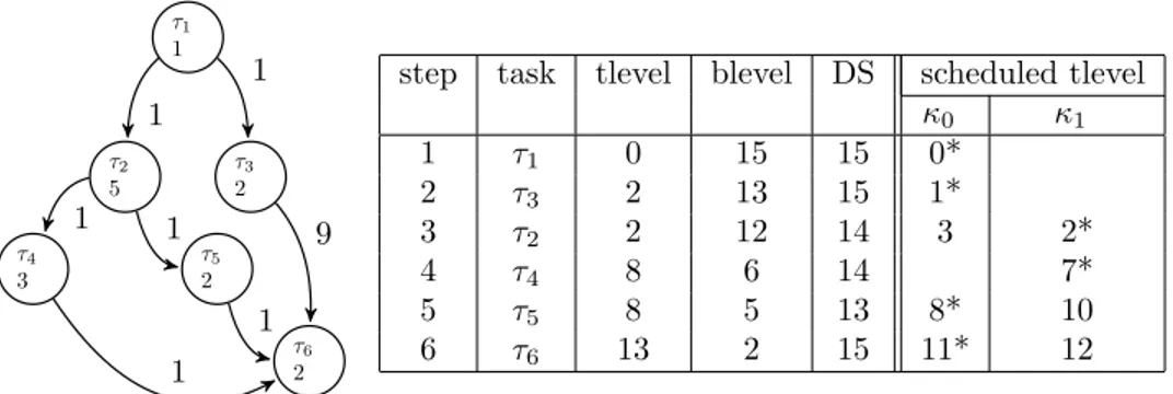
To illustrate the importance of this heuristic, suppose we have the DAG presented in Figure 3. Table 4 exhibits the difference in scheduling obtained by DSC and our extension on this graph. We observe here that the number of clusters generated using DSC is 3, with 5 idle slots, while BDSC needs only 2 clusters, with 2 idle slots. Moreover, BDSC achieves a better load balancing than DSC, since it reduces the variance of the clusters’ execution loads, defined, for a given cluster, as the sum of the costs of all its tasks: 0.25, for BDSC, vs. 6, for DSC. Finally, with our efficient task-to-cluster mapping, in addition to decreasing the number of generated clusters, we gain also in the total execution time. Indeed, our approach reduces communication costs by allocating tasks to the same cluster; for example, as shown in Figure 4, the total execution time with DSC is 14, but is equal to 13 with BDSC.
To get a feeling for the way BDSC operates, we detail the steps taken to get this better scheduling in the table of Figure 3. BDSC is equivalent to DSC until Step 5, where κ0 is chosen by our cluster mapping heuristic, since
τ1 1 τ2 5 τ3 2 τ4 3 τ5 2 τ6 2 1 1 1 1 1 9 1
step task tlevel blevel DS scheduled tlevel
κ0 κ1 1 τ1 0 15 15 0* 2 τ3 2 13 15 1* 3 τ2 2 12 14 3 2* 4 τ4 8 6 14 7* 5 τ5 8 5 13 8* 10 6 τ6 13 2 15 11* 12
Figure 3: A DAG amenable to cluster minimization (left) and its BDSC step-by-step schedul-ing (right) κ0 κ1 κ2 total time τ1 1 τ3 τ2 7 τ4 τ5 10 τ6 14 κ0 κ1 total time τ1 1 τ3 τ2 7 τ5 τ4 10 τ6 13
Figure 4: DSC (left) and BDSC (right) cluster allocations and execution times
successors(τ3, G) ⊂ successors(τ5, G); no new cluster needs to be allocated. 3.5. The BDSC Algorithm
BDSC extends the list scheduling template provided in Algorithm 1 by taking into account the various extensions discussed above. In a nutshell, the BDSC select cluster function, which decides in which cluster κ a task τ should be allocated, tries successively the four following strategies:
1. choose κ among the clusters of τ ’s predecessors that decrease the start time of τ , under MCW and DSRW constraints;
2. or, assign κ using our efficient task-to-cluster mapping strategy, under the additional constraint MCW;
3. or, create a new cluster if the PCW constraint is satisfied;
4. otherwise, choose the cluster among all clusters in M CW clusters min under the constraint MCW. Note that, in this worst case scenario, the tlevel of τ can be increased, leading to a decrease in performance since the length of the graph critical path is also increased.
BDSC is described in Algorithms 8 and 9; the entry graph Gu is the whole unscheduled program DAG, P , the maximum number of processors, and M , the maximum amount of memory available in a cluster. U T denotes the set of unexamined tasks at each BDSC iteration, RL, the set of ready tasks and U RL, the set of unready ones. We schedule the vertices of G according to the four rules above in a descending order of the vertices’ priorities. Each time a task
τr has been scheduled, all the newly readied vertices are added to the set RL (ready list) by the update ready set function.
BDSC returns a scheduled graph, i.e., an updated graph where some zeroings may have been performed and for which the clusters function yields the clusters needed by the given schedule; this schedule includes, beside the new graph, the cluster allocation function on tasks, cluster. If not enough memory is available, BDSC returns the original graph, and signals its failure by setting clusters to the empty set.
We suggest to apply here an additional heuristic, in that, if multiple vertices have the same priority, the vertex with the greatest bottom level is chosen for τr (likewise for τu) to be scheduled first to favor the successors that have the longest path from τrto the exit vertex. Also, an optimization could be performed when calling update priority values(G); indeed, after each cluster allocation, only the tlevels of the successors of τrneed to be recomputed instead of those of the whole graph.
Theorem 1. The time complexity of Algorithm 8 (BDSC) is O(n3), n being
the number of vertices in Graph G.
Proof. In the “while” loop of BDSC, the most expensive computation is the function end idle cluster used in f ind cluster that locates an existing cluster suitable to allocate there Task τ ; such reuse intends to optimize the use of the limited of processors. Its complexity is proportional to
X τκ∈vertices(G)
|successors(τκ, G)|,
which is of worst case complexity O(n2). Thus the total cost for n iterations of the “while” loop is O(n3).
Even though BDSC’s worst case complexity is larger than DSC’s, which is O(n2log(n)) [5], it remains polynomial, with a small exponent. Our experiments (see Section 5) showed this theoretical slowdown is indeed not a significant factor in practice.
4. BDSC-Based Hierarchical Parallelization
In this section, we detail how BDSC can be used, in practice, to schedule applications. We show how to build from an existing program source code what we call a Sequence Dependence Graph (SDG), which will play the role of DAG G above, how to then generate the numerical cost of vertices and edges in SDGs and how to perform what we call Hierarchical Scheduling (HBDSC) for SDGs. We use PIPS to illustrate how these new ideas can be integrated in an optimizing compilation platform.
PIPS [7] is a powerful, source-to-source compilation framework initially de-veloped at MINES ParisTech in the 1990s. Thanks to its open-source nature, PIPS has been used by multiple partners over the years for analyzing and trans-forming C and Fortran programs, in particular when targeting vector, parallel
ALGORITHM 8:BDSC scheduling Graph Gu, under processor and memory bounds P and M
function BDSC( Gu, P , M ) i f ( P ≤ 0 ) then
return error(′
Not enough processors′
, Gu) ; G = graph_copy ( Gu) ;
foreach τi ∈ vertices ( G )
priority( τi) = tlevel ( τi, G ) + blevel ( τj, G ) ; UT = vertices ( G ) ; RL = {τ ∈ UT / predecessors ( τ , G ) = ∅ } ; URL = UT − RL ; clusters = ∅ ; while UT 6= ∅ τr = select_task_with_highest_priority ( RL ) ; ( τm, min_tlevel ) = tlevel_decrease ( τr, G ) ; i f ( τm 6= τr ∧ MCW ( τr, cluster ( τm) , M ) ) then
τu = select_task_with_highest_priority ( URL ) ; i f ( priority ( τr) < priority ( τu) ) then
i f ( ¬DSRW ( τr, τu, clusters , G ) ) then i f ( PCW ( clusters , P ) ) then
κ = new_cluster ( clusters ) ;
allocate_task_to_cluster( τr, κ , G ) ; e l s e
i f ( ¬find_cluster ( τr, G , clusters , P , M ) ) then return error(′
Not enough memory′ , Gu) ; e l s e
allocate_task_to_cluster( τr, cluster ( τm) , G ) ; edge_cost( τm, τr) = 0 ;
e l s e i f ( ¬find_cluster ( τr, G , clusters , P , M ) ) then return error(′
Not enough memory′ , Gu) ; update_priority_values( G ) ; UT = UT−{τr} ; RL = update_ready_set ( RL , τr, G ) ; URL = UT−RL ; clusters( G ) = clusters ; return G; end
and hybrid architectures. Its advanced static analyses provide sophisticated in-formation about possible program behaviors, including use-def chains, precondi-tions, transformers, in-out array regions and worst-case code complexities. All information within PIPS is managed via specific APIs that are automatically provided from data structure specifications written with the Newgen domain specific language [10].
ALGORITHM 9:Attempt to allocate cluster in clusters for Task τ in Graph G, under processor and memory bounds P and M, returning true if successful
function find_cluster( τ , G , clusters , P , M ) MCW_idle_clusters = {κ ∈ end_idle_clusters ( τ , G , clusters , P ) / MCW( τ , κ , M ) } ; i f ( MCW_idle_clusters 6= ∅ ) then κ = choose_any ( MCW_idle_clusters ) ; allocate_task_to_cluster( τ , κ , G ) ; e l s e i f ( PCW ( clusters , P ) ) then
allocate_task_to_cluster( τ , new_cluster ( clusters ) , G ) ; e l s e
MCW_clusters = {κ ∈ clusters / MCW ( τ , κ , M ) } ;
MCW_clusters_min = argminκ ∈ MCW clusters cluster_time( κ ) ; i f ( MCW_clusters_min 6= ∅ ) then κ = choose_any ( MCW_clusters_min ) ; allocate_task_to_cluster( τ , κ , G ) ; e l s e return false; return true; end function error( m , G ) clusters( G ) = ∅ ; return G; end
4.1. Hierarchical Sequence Dependence DAG Mapping
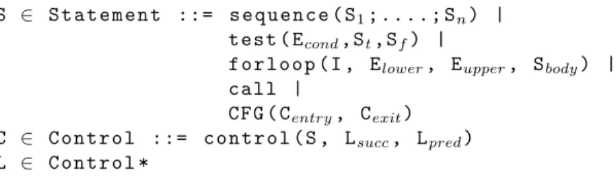
PIPS represents user code as abstract syntax trees. We define a subset of its grammar in Figure 5, limited to the statements S at stake in this paper. Econd, Elower and Eupperare expressions, while I is an identifier. The semantics of these constructs is straightforward. Note that, in PIPS, assignments are seen as function calls, where left hand sides are parameters passed by reference. We use the notion of control flow graph CFG to represent parallel code.
We assume that each task τ includes a statement S = task statement(τ ), which corresponds to the code it runs when scheduled.
In order to partition into tasks real applications, which include loops, tests and other structured constructs5, into dependence DAGs, our approach is to first build a Sequence Dependence DAG (SDG) which will be the input for the BDSC algorithm. Then, we use the code presented in form of an AST to define a
5
In this paper, we only handle structured parts of a code, i.e., the ones that do not contain gotostatements. Therefore, within this context, PIPS implements control dependences in its IR since it is equivalent to an AST (for structured programs, CDG and AST are equivalent).
S ∈ Statement ::= sequence ( S1;....; Sn) | test ( Econd,St,Sf) |
forloop (I , Elower, Eupper, Sbody) | call |
CFG ( Centry, Cexit)
C ∈ Control ::= control (S , Lsucc, Lpred)
L ∈ Control *
Figure 5: Abstract syntax tree Statement syntax
hierarchical mapping function, that we call H, to map each sequence statement of the code to its SDG. H is used for the input of the HBDSC algorithm. We present in this section what SDGs are and how an H is built upon them. 4.1.1. Sequence Dependence DAG
A Sequence Dependence DAG (SDG) G is a data dependence DAG where task vertices τ are labeled with statements, while control dependences are en-coded in the abstract syntax trees of statements. Any statement S can label a DAG vertex, i.e. each vertex τ contains a statement S, which corresponds to the code it runs when scheduled. We assume that there exist two functions vertex statement and statement vertex such that, on their respective domains of definition, they satisfy S = vertex statement(τ ) and statement vertex(S,G) = τ . In contrast to the usual program dependence graph defined in [11], an SDG is thus not built only on simple instructions, represented here as call statements; compound statements such as test statements (both true and false branches) and loop nests may constitute indivisible vertices of the SDG.
To compute the SDG G for a sequence S = sequence(S1; S2; ...; Sm), one may proceed as follows. First, a vertex τifor each statement Si in S is created; for loop and test statements, their inner statements are recursively traversed and transformed into SDGs. Then, using the Data Dependence Graph D, de-pendences coming from all the inner statements of each Si are gathered to form cumulated dependences. Finally, for each statement Si, we search for other statements Sj such that there exists a cumulated dependence between them and add a dependence edge (τi,τj) to G. G is thus the quotient graph of D with respect to the dependence relation.
Figure 7 illustrates the construction, from the DDG given in Figure 6 (right), the SDG of the C code (left). The figure contains two SDGs corresponding to the two sequences in the code; the body S0 of the first loop (in blue) has also an SDG G0. Note how the dependences between the two loops have been deduced from the dependences of their inner statements (their loop bodies). These SDGs and their printouts have been generated automatically with PIPS.
void main () { int a [11] , b [11]; int i ,d , c ; // S { c =42; for ( i =1; i <=10; i ++) { a [ i ] = 0; } for ( i =1; i <=10; i ++) { // S0 a [ i ] = bar ( a [ i ]) ; d = foo ( c ) ; b [ i ] = a [ i ]+ d ; } } return ; }
Figure 6: Example of a C code (left) and the DDG D of its internal S sequence (right, where red denotes true data-flow dependences, blue, output dependences, and green, anti-dependences)
4.1.2. Hierarchical SDG Mapping
We presented above how sequences of statements can be transformed into SDGs. This section suggests to handle the other types of statements, such as loops and tests, by adopting a hierarchical view of the source code, encoded in a new data structure. A hierarchical SDG mapping function H maps each statement S to an SDG G = H(S) if S is a sequence statement; otherwise G is equal to ⊥. In the figure 7 we already saw, a hierarchical SDG mapping H is illustrated. Here, H(S) is G, while, for the SDG G0 corresponding to the body S0 of the loop, one has G0 = H(S0). These SDGs have been generated automatically with PIPS; we use the Graphviz tool for pretty printing [12].
Our introduction of the notions of SDGs and hierarchical mappings is moti-vated by the following observations, which also support our design decisions:
1. The true and false statements of a test are control dependent upon the condition of the test statement, while every statement within a loop (i.e., statements of its body) is control dependent upon the loop statement
Figure 7: SDGs of S (top) and S0 (bottom) computed from the DDG (see the right of Figure 6); S and S0 are specified in the left of Figure 6
header. If we define a control area as a set of statements transitively linked by the control dependence relation, our SDG construction process insures that the control area of the statement of a given vertex is in the vertex. This way, we keep all the control dependences of a task in our SDG within itself.
2. We decided to consider test statements as single vertices in the SDG to ensure that they are scheduled on one cluster6, which guarantees the ex-ecution of the inner code (true or false statements), whichever branch is taken, on this cluster.
3. We do not group successive simple call instructions into a single “basic block” vertex in the SDG in order to let BDSC fuse the corresponding statements so as to maximize parallelism and minimize communications. Note that PIPS performs interprocedural analyses, which will allow call sequences to be efficiently scheduled whether these calls represent trivial assignments or complex function calls.
6
4.2. Cost Models Generation
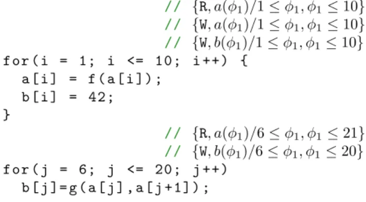
Since the volume of data used or communicated by SDG tasks are key fac-tors in the BDSC scheduling process, we need to as precisely as possible assess this information. PIPS provides an intra- and inter-procedural analysis of array data flow called regions analysis [13] that computes dependences for each array element access. Sets of array elements are gathered into array regions, which are represented by convex polyhedra expressions over the variables values in the current memory store. For each statement S, two types of sets R of regions r are considered in this paper: read regions(S) and write regions(S) contain the array elements respectively read and written by S. The two types of regions are distinguished by a label, either R or W. For instance, in Figure 8, PIPS is able to infer sets of regions such as:
Rwa= {W, a(φ1)/1 ≤ φ1, φ1≤ 10} Rra= {R, a(φ1)/6 ≤ φ1, φ1≤ 21}
where the write regions Rwaof Array a, modified in the first loop, are the array elements of a with indices in the interval [1,10]. The read regions Rra of Array a in the second loop represents the elements with indices in [6,21].
// {R, a(φ1)/1 ≤ φ1, φ1≤ 10} // {W, a(φ1)/1 ≤ φ1, φ1≤ 10} // {W, b(φ1)/1 ≤ φ1, φ1≤ 10} for ( i = 1; i <= 10; i ++) { a [ i ] = f ( a [ i ]) ; b [ i ] = 42; } // {R, a(φ1)/6 ≤ φ1, φ1≤ 21} // {W, b(φ1)/6 ≤ φ1, φ1≤ 20} for ( j = 6; j <= 20; j ++) b [ j ]= g ( a [ j ] , a [ j +1]) ;
Figure 8: Example of array region analysis
4.2.1. From Convex Polyhedra to Ehrhart Polynomials
Our analysis uses the following operations on sets Ri of regions (convex polyhedra)7:
1. regions intersection(R1,R2) is a set of regions; each region r in this set is the intersection of two regions r1∈ R1 and r2∈ R2 referencing the same
7
Note that regions must be defined with respect to a common memory store for these operations to be properly defined.
array. The convex polyhedron of r is the intersection of the two convex polyhedra of r1and r2, which is also a convex polyhedron.
2. regions union(R1,R2) is a set of regions; each region r in this set is the union of two regions r1 ∈ R1 and r2 ∈ R2 with the same reference. The convex polyhedron of r is the union of the two convex polyhedra of r1 and r2, which is not necessarily a convex polyhedron. An approximated convex hull is thus computed in order to return the smallest enclosing polyhedron.
Since we are interested in the size of these regions to precisely assess communi-cation costs and memory requirements, we compute Ehrhart polynomials [14], which represent the number of integer points contained in a given parameterized polyhedron, from this region. To manipulate these polynomials, we use various operations using the Ehrhart API provided by the polylib library [15].
Communication Edge Cost To assess the communication cost between two SDG vertices, τ1 as source and τ2 as sink vertices, we rely on the number of bytes involved in true data-flow dependences, of type “read after write” (RAW), using the read and write regions as follows:
Rw1 = write regions(vertex statement(τ1)) Rr2 = read regions(vertex statement(τ2))
edge cost bytes(τ1, τ2) =Pr∈regions intersection(Rw1,Rr2)ehrhart(r)
In practice, in our experiments (see Section 5), in order to compute nication times, this polynomial, which represents the message size to commu-nicate, expressed in number of bytes, is multiplied by the transfer time of one byte (β), to which is then added the latency time (α). These two coefficients are dependent on the specific target machine. We note:
edge cost(τ1, τ2)= α + β × edge cost bytes(τ1, τ2)
Local Storage Task Data To provide an estimation of the volume of data used by each vertex τ , we use the number of bytes of data read and written by the task statement, via the following definitions :
S = task statement(τ );
task data(τ ) = data merge(read regions(S), write regions(S)) where we define data merge and data size as follows:
data merge(R1, R2) = regions union(R1, R2) data size(R) =Pr∈Rehrhart(r)
Execution Task Time In order to determine an average execution time for each vertex in the SDG, we use a static execution time approach based on a program complexity analysis provided by PIPS. There, each statement S is automatically labeled with an expression, represented by a polynomial over program variables complexity estimation(S), that denotes an estimation of the
execution time of this statement, assuming that each basic operation (addition, multiplication...) has a fixed, architecture-dependent execution time. This so-phisticated static complexity analysis is based on inter-procedural information such as preconditions. Using this approach, one can define task time as:
task time(τ ) = complexity estimation(task statement(τ )) 4.2.2. From Polynomials to Values
We have just seen how to represent cost, data and time information in terms of polynomials; yet, running BDSC requires actual values. This is particularly a problem when computing tlevels and blevels, since cost and time are cumulated there. We decided to convert cost information into time by assuming that communication times are proportional to costs, which amounts in particular to setting communication latency to zero8.
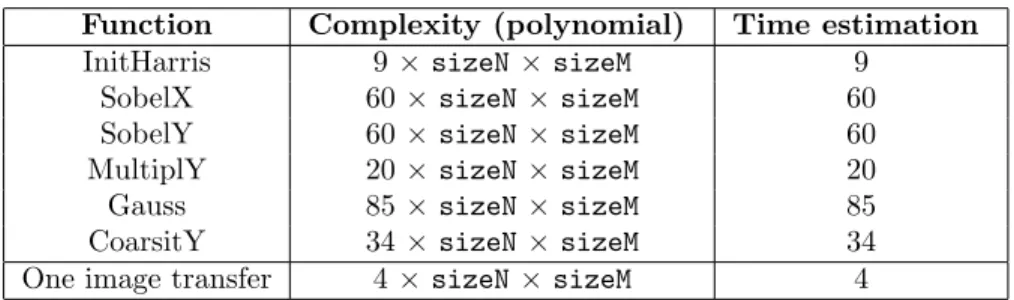
When program variables used in the above-defined polynomials are numer-ical values, each polynomial is a constant; this happens to be the case for one of our applications, ABF. However, when input data are unknown at compile time (as for the Harris application), we suggest to use a very simple heuristic to approximate the values of the polynomials. When all polynomials at stake are monomials on the same base, we simply keep the coefficient of these monomials. Even though this heuristics appears naive at first, it actually is quite useful in the Harris application: Table 1 shows the complexities and time estimation generated for each function of Harris using PIPS default operation cost model, where the sizeN and sizeM variables represent the input image size.
Function Complexity (polynomial) Time estimation
InitHarris 9 × sizeN × sizeM 9
SobelX 60 × sizeN × sizeM 60
SobelY 60 × sizeN × sizeM 60
MultiplY 20 × sizeN × sizeM 20
Gauss 85 × sizeN × sizeM 85
CoarsitY 34 × sizeN × sizeM 34
One image transfer 4 × sizeN × sizeM 4
Table 1: Execution and communication time estimations for Harris using PIPS default cost models
The general case deals with polynomials that are functions of many variables, as is the case in equake, where they depend on variables such as ARCHelems or ARCHnodes. In such cases, we suggest to first instrument the input sequential code and run it once in order to obtain the numerical values of the polynomi-als. The instrumented code contains the initial user code plus instructions that compute the values of the cost polynomials for each statement. BDSC is then
8
This assumption is validated by our experimental results, and the fact that our data arrays are large.
applied, using this cost information, to yield the final parallel program. Note that this approach is sound since BDSC ensures that the value of a variable (and thus a polynomial) is the same, whichever scheduling is used. Of course, this approach will work well, as our experiments suggest, when a program per-formance does not change when some part of its input parameters are modified; this is the case for many signal processing applications, where performance is mostly a function of structure parameters such as image size, and is independent of the actual signal (pixel) values upon which the program acts.
We show an example of this final case using a part of the instrumented equake code9 in Figure 9. The added instrumentation instructions are fprintf statements, the second parameter of which represents the statement number of the following statement, and the third, the value of its execution time for task time instrumentation. For edge cost instrumentation, the second parameter is the number of the incident statements of the edge, and the third, the edge cost polynomial. After execution of the instrumented code, the numerical results of the polynomials are printed in the file instrumented equake.in. This file will be an entry for the PIPS implementation of BDSC.
FILE ∗ finstrumented = fopen("instrumented equake.in", "w"); fprintf (finstrumented,
"task time 62 = %ld\n", 179 ∗ ARCHelems + 3); for ( i = 0; i < A R C H e l e m s ; i ++) {
for ( j = 0; j < 4; j ++) cor [ j ] = A R C H v e r t e x [ i ][ j ]; }
fprintf (finstrumented,
"task time 163= %ld\n", 20 ∗ ARCHnodes + 3); for ( i = 0; i <= ARCHnodes -1; i += 1)
for ( j = 0; j <= 2; j += 1) disp [ d i s p t p l u s ][ i ][ j ] = 0.0; fprintf (finstrumented,
"edge cost 163 → 166 = %ld\n", ARCHnodes ∗ 9); fprintf (finstrumented,
"task time 166= %ld\n", 110 ∗ ARCHnodes + 106); s m v p _ o p t ( ARCHnodes , K ,
ARCHmatrixcol , AR C Hm a tr i xi nd e x , disp [ dispt ] , disp [ d i s p t p l u s ]) ;
Figure 9: Excerpt of instrumented equake (S0 is the inner loop sequence)
9
We do not show the instrumentation on the statements inside the loops for readability purposes.
4.3. Hierarchical Scheduling (HBDSC)
Now that all the information needed by the basic version of BDSC presented above has been gathered, we detail in Algorithm 10 how we suggest to adapt it to different SDGs linked hierarchically via the mapping function H introduced above in order to eventually generate nested parallel code when possible. We adopt in this section the graph-based parallel programming model since it offers the freedom to implement arbitrary parallel patterns and since SDGs implement this model. Therefore, we use the CFG construct of the PIPS IR to encode the generated parallel code.
4.3.1. Recursive Top-Down Scheduling
Hierarchically scheduling a given statement S of SDG H(S) in a cluster κ is seen here as the definition of a hierarchical schedule σ which maps each inner statement s of S to σ(s) = (s′, κ, n). If there are enough processor and memory resources to schedule S using BDSC, (s′, κ, n) is a triplet made of a parallel statement s′ = parallel(σ(s)), the cluster κ = cluster(σ(s)) where s is being allocated and the number n = nbclusters(σ(s)) of clusters the inner scheduling of s′ requires. Otherwise, scheduling is impossible, and the program stops. In a scheduled statement, all sequences are replaced by parallel CFG statements.
A successful call to the HBDSC(S, H, κ, P, M, σ) function defined in Algo-rithm 10, which assumes that P is strictly positive, yields a new version of σ that schedules S into κ and takes into account all inner statements of S; only P clusters, with a data size at most M each, can be used for scheduling. σ[S → (S′, κ, n)] is the function equal to σ except for S, where its value is (S′, κ, n). H is the function that yields an SDG for each S to be scheduled using BDSC.
Our approach is top-down in order to yield tasks that are as coarse grained as possible when dealing with sequences. In the HBDSC function, we distin-guish four cases of statements. First, the constructs of loops10 and tests are simply traversed, scheduling information being recursively gathered in different SDGs. Then, for a call statement, there is no descent in the call graph, the call statement is returned. In order to handle the corresponding call function, one has to treat separately the different functions. Next, for a sequence S, one first accesses its SDG and computes a closure of this DAG, Gseq, using the function closure. The purpose of the closure function (see [16]) is to provide a self-contained version of H(S): H(S) is completed with a set of entry vertices and edges in order to represent the dependences coming from outside S, yield-ing the closed SDG Gseq. Finally, Gseq is scheduled using BDSC to generate a scheduled SDG G′.
10
Regarding parallel loops, since we adopt the task parallelism paradigm, note that, initially, it may be useful to apply the tiling transformation and then perform full unrolling of the outer loop (we give more details in the protocol of our experiments in Section 5.1). This way, the input code contains more potentially parallel tasks resulting from the initial (parallel) loop.
ALGORITHM 10: BDSC-based update of Schedule σ for Statement S of SDG H(S), with P and M constraints
function HBDSC( S , H , κ , P , M , σ ) switch ( S ) case call: return σ[ S → ( S , κ , 0 ) ] ; case sequence( S1; . . . ; Sn) : Gseq = closure ( S , H ( S ) ) G′ = BDSC ( Gseq, P , M , σ ) ; iter = 0 ; do σ′ = HBDSC_step ( G′, H , κ , P , M , σ ) ; G = G′ ; G′ = BDSC ( Gseq, P , M , σ′ ) ; i f ( clusters ( G′ ) = ∅ ) then abort(′ Unable to schedule′ ) ; iter++; σ = σ′ ; while ( completion_time ( G′ ) < completion_time ( G ) ∧ | clusters ( G′ ) | ≤ | clusters ( G ) | ∧ iter ≤ MAX_ITER )
return σ[ S → ( dag_to_cfg ( G ) , κ , | clusters ( G ) | ) ] ; case forloop( I , Elower, Eupper, Sbody) :
σ′
= HBDSC ( Sbody, H , κ , P , M , σ ) ; ( S′
body, κbody, nbclustersbody) = σ ′
( Sbody) ; return σ′
[ S → ( forloop ( I , Elower, Eupper, S′ body) , κ, nbclustersbody) ] ;
case test( Econd, St, Sf) : σ = HBDSC ( St, H , κ , P , M , σ′ ) ; σ′′ = HBDSC ( Sf, H , κ , P , M , σ′ ) ; ( S′ t, κt, nbclusterst) = σ ′′ ( St) ; ( S′ f, κf, nbclustersf) = σ ′′ ( Sf) ; return σ′′ [ S → ( test ( Econd, S′ t, S ′ f) ,
κ, max ( nbclusterst, nbclustersf) ) ] ; end
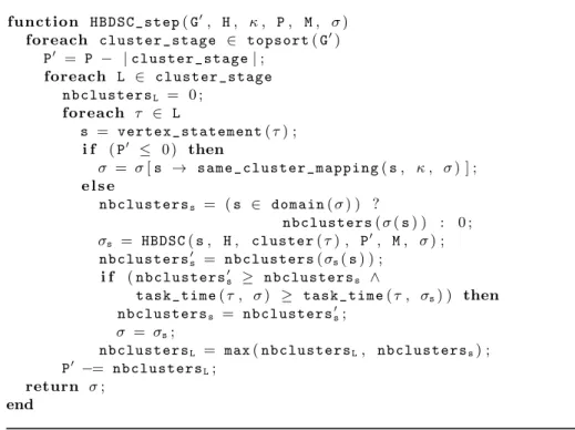
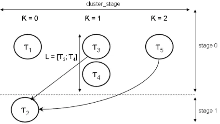
The hierarchical scheduling process is then recursively performed, to take into account inner statements of S, within Function HBDSC step defined in Algorithm 11 on each statement s of each task of G′
. There, G′
is traversed along a topological sort-ordered descent using the function topsort(G′
) yields a list of stages of computation, each cluster stage being a list of independent lists L of tasks τ , one L for each cluster κ generated by BDSC for this particular stage in the topological order.
The recursive hierarchical scheduling via the function HBDSC, within the function HBDSC step, of each statement s = vertex statement(τ ) may take
ad-vantage of at most P′available clusters, since |cluster stage| clusters are already reserved to schedule the current stage cluster stage of tasks for Statement S. It yields a new scheduling function σs. Otherwise, if no clusters are available, all inner statements of s are scheduled on the same cluster as their parent, κ. We use the straightforward function same cluster mapping (not provided here) to affect recursively (se, κ, 0) to σ(se) for each inner se of s.
ALGORITHM 11:Iterative hierarchical scheduling step for DAG fixpoint compu-tation
function HBDSC_step( G′, H , κ , P , M , σ ) foreach cluster_stage ∈ topsort ( G′
) P′ = P − | cluster_stage | ; foreach L ∈ cluster_stage nbclustersL = 0 ; foreach τ ∈ L s = vertex_statement ( τ ) ; i f ( P′ ≤ 0 ) then σ = σ [ s → same_cluster_mapping ( s , κ , σ ) ] ; e l s e nbclusterss = ( s ∈ domain ( σ ) ) ? nbclusters( σ ( s ) ) : 0 ; σs = HBDSC ( s , H , cluster ( τ ) , P ′ , M , σ ) ; nbclusters′ s = nbclusters ( σs( s ) ) ; i f ( nbclusters′ s ≥ nbclusterss ∧
task_time( τ , σ ) ≥ task_time ( τ , σs) ) then nbclusterss = nbclusters′
s; σ = σs;
nbclustersL = max ( nbclustersL, nbclusterss) ; P′
−= nbclustersL; return σ;
end
Figure 10 illustrates the various entities involved in the computation of such a scheduling function. Note that one needs to be careful in HBDSC step to ensure that each rescheduled inner statement s is allocated a number of clusters consistent with the one used when computing its parallel execution time; we check the condition nbclusters′
s ≥ nbclusterss, which ensures that the paral-lelism assumed when computing time complexities within s remains available.
Cluster allocation information for each inner statement s whose vertex in G′ is τ is maintained in σ via the recursive call to HBDSC, this time with the current cluster κ = cluster(τ ). For the non-sequence constructs in Function HBDSC, cluster information is set to κ, the current cluster.
The scheduling of a sequence yields a parallel CFG statement; we use the function dag to cfg(G) that returns a PIPS control flow graph statement Scf g from the SDG G, where the vertices of G are the statement control vertices
Figure 10: topsort(G) for the hierarchical scheduling of sequences
scf g of Scf g, and the edges of G constitute the list of successors Lsucc of scf g while the list of predecessors Lpred of scf g is deduced from Lsucc. Note that vertices and edges of G are not changed before and after scheduling; however, information of scheduling is saved in σ.
4.3.2. Iterative Scheduling for Resource Optimization
BDSC is called in HBDSC before inner statements are hierarchically sched-uled. However, a unique pass over inner statements could be suboptimal, since parallelism may exist within inner statements. It may be discovered by later recursive calls to HBDSC. Yet, if this parallelism had been known ahead of time, previous values of task time used by BDSC would have been possibly smaller, which could have had an impact on the higher-level scheduling. In or-der to address this issue, our hierarchical scheduling algorithm iterates the top
down pass HBDSC step on the new DAG G′ in which BDSC takes into account
these modified task complexities; iteration continues while G′provides a smaller DAG schedule length than G and the iteration limit MAX ITER has not been reached. We compute the completion time of the DAG G, as follows:
completion time(G) = maxκ∈clusters(G)cluster time(κ)
One constraint due to the iterative nature of the hierarchical scheduling is that, in BDSC, zeroing cannot be made between the entry vertices and their successors. This keeps an independence in terms of allocated clusters between the different levels of the hierarchy. Indeed, at a higher level, for S, if we assume that we have scheduled the parts Se inside (hierarchically) S; attempting to reschedule S iteratively cancels the precedent schedule of S but maintains the schedule of Se and vice versa. Therefore, for each sequence, we have to deal with a new set of clusters; and thus, zeroing cannot be made between these entry vertices and their successors.
Note that our top-down, iterative,e hierarchical scheduling approach also helps dealing with limited memory resources. If BDSC fails at first because not enough memory is available for a given task, the HBDSC step function
is nonetheless called to schedule nested statements, possibly loosening up the memory constraints by distributing some of the work on less memory-challenged additional clusters. This might enable the subsequent call to BDSC to succeed. 4.3.3. Parallel Cost Models
In Section 4.2, we present the sequential cost models usable in the case of sequential codes, i.e, for each first call to BDSC. When an inner statement Se of S is parallelized, the parameters task time, task data and edge cost are modified for Seand thus for S. Thus, hierarchical scheduling must use extended definitions of task time, task data and edge cost for tasks τ using statements S = vertex statement(τ ) that are CFG statements, extending the definitions provided in Section 4.2, which still apply to non-CFG statements. For such a case, we assume that BDSC and other relevant functions take σ as an additional argument to access the scheduling result associated to statement sequences and handle the modified definitions of task time, edge cost and task data. These functions can be found in [16].
4.3.4. Complexity of HBDSC Algorithm
Theorem 2. The time complexity of Algorithm 10 (HBDSC) over Statement S is O(kn), where n is the number of call statements in S and k a constant greater than 1.
Proof. Let t(l) be the worst-case time complexity for our hierarchical scheduling algorithm on the structured statement S of hierarchical level11 l. Time com-plexity increases significantly only in sequences, loops and tests being simply managed by straightforward recursive calls of HBDSC on inner statements. For a sequence S, t(l) is proportional to the time complexity of BDSC followed by a call to HBDSC step; the proportionality constant is k =MAX ITER (supposed to be greater than 1).
The time complexity of BDSC for a sequence of m statements is at most
O(m3) (see Theorem 1). Assuming that all subsequences have a maximum
number m of (possibly compound) statements, the time complexity for the hierarchical scheduling step function is the time complexity of the topological sort algorithm followed by a recursive call to HBDSC, and is thus O(m2 + mt(l − 1)). Thus t(l) is at most proportional to k(m3+ m2+ mt(l − 1)) ∼ km3+ kmt(l − 1). Since t(l) is an arithmetico-geometric series, its analytical value t(l) is (km) l (km3 +km−1)−km3 km−1 ∼ (km) lm2. Let l
S be the level for the whole Statement S. The worst performance occurs when the structure of S is flat, i.e., when lS ∼ n and m is O(1); hence t(n) = t(lS) ∼ kn.
Even though the worst case time complexity of HBDSC is exponential, we expect and our experiments suggest that it behaves more tamely on actual, properly structured code. Indeed, note that lS ∼ logm(n) if S is balanced for
11
Levels represent the hierarchy structure between statements of the AST and are counted up from leaves to the root.
some large constant m; in this case, t(n) ∼ (km)log(n), showing a subexponential time complexity.
5. Experiments
The BDSC algorithm presented in this paper has been designed to offer better task parallelism extraction performance for parallelizing compilers than traditional list-scheduling techniques such as DSC. To verify its effectiveness, BDSC has been implemented in PIPS and tested on actual applications written in C. In this section, we provide preliminary experimental BDSC-vs-DSC com-parison results based on the parallelization of four such applications, namely ABF, Harris, equake and IS. We chose these particular applications since they are well-known benchmarks and exhibit task parallelization that we hope our approach will be able to take advantage of. They are: (1) ABF (Adaptive Beam Forming), a 1,065-line program that performs adaptive spatial radar signal pro-cessing [17]; (2) Harris, a 105-line image propro-cessing corner detector [18]; (3) the 1,432-line SPEC benchmark equake [19], which is used in the finite element simulation of seismic wave propagation; and (4) Integer Sort (IS), one of the eleven benchmarks in the NAS Parallel Benchmarks suite [20], with 1,076 lines. 5.1. Protocol
We have extended PIPS with our implementation in C of BDSC-based hierar-chical scheduling. To compute the static execution time and communication cost estimates needed by BDSC, we relied upon the PIPS run time complexity anal-ysis and a more realistic, architecture-dependent communication cost matrix (Table 1 was computed using the simpler PIPS default cost models). For each code S of our four test application, PIPS performed automatic parallelization, applying our hierarchical scheduling process hierarchical schedule(S, P, M, ⊥) (using either BDSC or DSC) on these sequential programs to yield σ. PIPS automatically generated an OpenMP [21] version from the scheduled SDGs in σ(S), using omptask directives; another version, in MPI [22], was generated from the scheduled SDGs. We also applied DSC in the hierarchical schedul-ing process of these applications and generated the correspondschedul-ing OpenMP and MPI codes. Compilation times for these applications were quite reasonable, the longest (equake) being 84 seconds. In this last instance, most of the time (79 seconds) was spent by PIPS to gather semantic information such as regions, complexities and dependences; our prototype implementation of BDSC is only responsible for the remaining 5 seconds.
We ran all these parallelized codes on two shared and distributed memory computing systems. To increase available coarse-grain task parallelism in our test suite, we have used both unmodified and modified versions of our applica-tions. We tiled and fully unrolled the four most costly loops in ABF and equake; the tiling factor for the BDSC version is the number of available processors, while we had to find the proper one for DSC, since DSC puts no constraints on the number of needed processors but returns the number of processors its
scheduling requires. For Harris and IS, our experiments have looked at both tiled and untiled versions of the applications.
5.2. Experiments on Shared Memory Systems
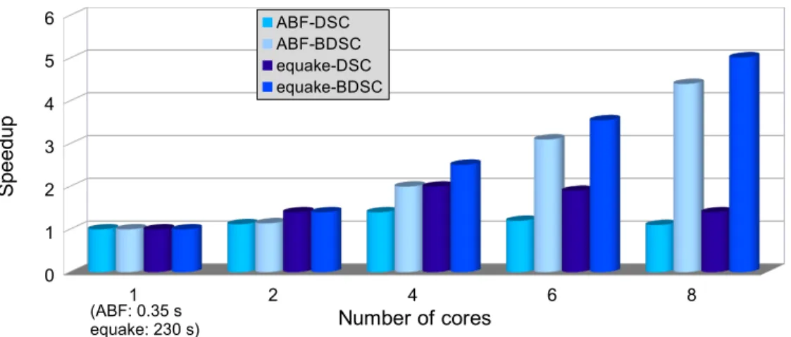
We measured the execution time of the parallel OpenMP codes on the P = 1, 2, 4, 6 and 8 cores of a host Linux machine with a 2-socket AMD quad-core Opteron with 8 quad-cores, with M = 16 GB of RAM, running at 2.4 GHz. Figure 11 shows the performance results of the generated OpenMP code on the two versions scheduled using DSC and BDSC on ABF and equake. The speedup data show that the DSC algorithm is not scalable, when the number of cores is increased; this is due to the generation of more clusters with empty slots than with BDSC, a costly decision given that, when the number of clusters exceeds P , they have to share the same core as multiple threads.
Figure 11 shows the performance results of the generated OpenMP code on the two versions scheduled using DSC and BDSC on ABF and equake. The speedup data show that the DSC algorithm is not scalable on these examples, when the number of cores is increased; this is due to the generation of more clusters (task creation overhead) with empty slots (poor potential parallelism and bad load balancing) than with BDSC, a costly decision given that, when the number of clusters exceeds P , they have to share the same core as multiple threads. 1 2 4 6 8 0 1 2 3 4 5 6 ABF-DSC ABF-BDSC equake-DSC equake-BDSC Number of cores S p e e d u p (ABF: 0.35 s equake: 230 s)
Figure 11: ABF and equake speedups with OpenMP
Figure 12 shows the hierachically scheduled SDG for Harris, generated auto-matically with PIPS using the Graphviz tool for three cores without tiling any loops (we used three cores because the maximum parallelism in Harris is three, as can be seen in the graph).
Figure 13 presents the speedup obtained using P = 3, since the maximum parallelism in Harris is three, assuming no exploitation of data parallelism,
Figure 12: Hierarchically scheduled SDG for Harris, using P =3 cores
for two parallel versions: BDSC with and BDSC without tiling of the kernel CoarsitY(we tiled by 3). The performance is given using three different input image sizes: 1024 × 1024, 2048 × 1024 and 2048 × 2048. The best speedup corresponds to the tiled version with BDSC because, in this case, the three cores are fully loaded. The DSC version (not shown in the figure) yields the same results as our versions because the code can be scheduled using three cores.
1024x1024 2048x1024 2048x2048 0 0.5 1 1.5 2 2.5 Harris-OpenMP Harris-tiled-OpenMP Image size S p e e d u p 3 t h re a d s v s . s e q u e n ti a l
sequential = 183 ms sequential = 345 ms sequential = 684 ms
Figure 13: Speedups with OpenMP: impact of tiling (P=3)
Figure 14 shows the performance results of the generated OpenMP code on the NAS benchmark IS after applying BDSC. The maximum task parallelism without tiling in IS is two, which is shown in the first subchart; the other subcharts are obtained after tiling. The program has been run with three IS input classes (A, B and C [20]). The bad performance of our implementation for Class A programs is due to the large task creation overhead, which dwarfs the potential parallelism gains, even more limited here because of the small size