HAL Id: hal-01086050
https://hal.archives-ouvertes.fr/hal-01086050
Submitted on 21 Nov 2014
HAL is a multi-disciplinary open access
archive for the deposit and dissemination of
sci-entific research documents, whether they are
pub-lished or not. The documents may come from
teaching and research institutions in France or
abroad, or from public or private research centers.
L’archive ouverte pluridisciplinaire HAL, est
destinée au dépôt et à la diffusion de documents
scientifiques de niveau recherche, publiés ou non,
émanant des établissements d’enseignement et de
recherche français ou étrangers, des laboratoires
publics ou privés.
Open licence - etalab|
EFFICIENT QUANTIZATION PARAMETER
ESTIMATION IN HEVC BASED ON ρ-DOMAIN
Thibaud Biatek, Mickaël Raulet, J.-F Travers, Olivier Deforges
To cite this version:
Thibaud Biatek, Mickaël Raulet, J.-F Travers, Olivier Deforges. EFFICIENT QUANTIZATION
PARAMETER ESTIMATION IN HEVC BASED ON ρ-DOMAIN. European Signal Processing
Con-ference (EUSIPCO), Sep 2014, Lisbonne, Portugal. �hal-01086050�
EFFICIENT QUANTIZATION PARAMETER ESTIMATION IN HEVC BASED ON ρ-DOMAIN
T. Biatek
∗, M. Raulet
†∗, J.-F. Travers
‡, O. Deforges
†∗
b<>com, Cesson-Sevigne, France
†IETR / INSA de Rennes, Rennes, France
‡
TDF, Cesson-Sevigne, France
ABSTRACT
This paper proposes a quantization parameter estimation algorithm for HEVC CTU rate control. Several methods were proposed, mostly based on Lagrangian optimization combined with Laplacian distribution for transformed coeffi-cients. These methods are accurate but increase the encoder complexity. This paper provides an innovative reduced com-plexity algorithm based on a ρ-domain rate model. Indeed, for each CTU, the algorithm predicts encoding parameters based on co-located CTU. By combining it with Laplacian distri-bution for transformed coefficients, we obtain the dead-zone boundary for quantization and the related quantization pa-rameter. Experiments in the HEVC HM Reference Software show a good accuracy with only a 3% average bitrate error and no PSNR deterioration for random-access configuration.
Index Terms— HEVC, Rate-Control, ρ-Domain
1. INTRODUCTION
High Efficiency Video Coding (HEVC) [1, 2] is the latest Video Coding Standard, standardized by the Joint Collabora-tive Team on Video Coding (JCT-VC) composed of experts from the ISO/IEC Moving Picture Experts Group (MPEG) and the ITU-T Video Coding Expert Group (VCEG). Due to telecommunication channels, bandwidth restrictions or storage capacity, rate-control plays an important part, and contains two major aspects. The first one relies on bit al-location, the algorithm has to break up the video signal at a particular granularity level (group of pictures, picture or piece of picture) and to wisely share the whole budget. The sec-ond one consists in reaching the previously allocated budgets while encoding. This is carried out by adjusting the quanti-zation parameter (QP). Indeed, the more you increase the QP, the more you lose information and the more you reduce bi-trate. Moreover, in high definition broadcasting environment, rate control algorithms have to fulfill real-time encoding re-strictions.
Several algorithms were proposed for HEVC rate-control. During standardization, [3] and [4] were proposed, based on particular rate models. In [3], the authors proposed a Rate-QP model, later replaced by [4], a more efficient algorithm based
on R-Lambda Model. This R-Lambda based algorithm is currently integrated into the HM Reference Software [5]. An-other approach for video coding rate control called ρ-Domain was introduced in [6], proposing a rate model linking ρ – the rate of non-zero coefficients after transformation and quantization– with the bitrate. This approach is interesting since it provides low-complexity linear modeling. Recently, this ρ-Domain approach was also investigated for the new HEVC Standard in [7] and [8]. These schemes are based on a model of Laplacian transformed coefficient distribution introduced in [9] and perform a picture level rate control. It is equally possible to perform rate-control at a lower level, since HEVC provides a block picture partioning called Cod-ing Tree Units (CTU). In [10] and [11], two CTU-based rate control algorithm are proposed. The first one is based on a quadratic rate modelisation and restrained to All-Intra con-figuration. The second one relies on a Laplacian distribution of transformed coefficients combined with a Lagrangian opti-mization problem. These approaches are accurate but do not take into account complexity issues, which is irrelevant for real-time encoding. In this paper, we propose a QP estimation scheme for HEVC, with the following innovative features:
• CTU-based prediction for encoding parameters. • CTU-based ρ-Domain modeling.
• Reduced complexity framework for Laplace parameter
estimation and Quantization parameter estimation. This paper is organized as follows. Section 2 provides a back-ground and discussions on ρ-Domain, Laplacian Distribution of transformed coefficients and on Lagrangian based meth-ods. In Section 3, the proposed method is presented, and the QP estimation scheme is provided. In Section 4, the experi-mental results are shown and discussed. Section 5 concludes this paper.
2. BACKGROUND AND DISCUSSION 2.1. HEVC Quadtree Partitioning
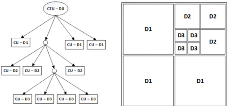
HEVC prodives an efficient quadtree partitioning, described in [12]. This partitioning defines a recursively structure called quadtree. The top of this quadtree contains the CTU, which can be subdivided into Coding Units (CU). Each of these CUs
can be subdivided again, until a depth limit is reached (depth = 3). For each CU, a Prediction Unit (PU) can be defined to mention information related to prediction. Another unit called Transform Unit (TU) and related to transformation can also be defined. In Figure 1, we can observe an example of partitioning in HEVC. This depth aspect is crucial since sev-eral encoding parameters will be collected and used per-depth in the proposed algorithm.
Fig. 1: An illustration of quadtree partitioning in HEVC, with a depth-3 recursive structure.
2.2. Laplacian Distribution
In [9], a particular mixture of Laplacian distribution for inter residual is provided. It was demonstrated that transformed coefficients are distributed separatly depending on the depth. In Equation 1, the Laplacian probability density function is defined with the distribution parameter λdepth. The variance
of a sample can be computed as σ2= 2/λ2depth
fdepth(x) = λdepth
2 ∗ e
−λdepth∗x (1)
In Figure 2-a, we can observe an example of multi-depth dis-tribution that is observed in HEVC. This disdis-tribution is rel-evant since the parameter computation through variance is known and simple.
2.3. Lagrange Multiplier
Several algorithms are based on Lagrange multiplier in or-der to minimize the perceived distorsion for a given targeted number of bits. This method comes under an unconstrained optimization problem (Equation 2) so as to minimize the rate distorsion cost J. The parameters are: the perceived distorsion D, the number of bit used R and the Lagrange multiplier Λ.
J = D + Λ∗ R (2)
This type of approach increases the algorithm complexity since it introduces the computation of visual quality met-rics. Thus, we avoid Lagrange multiplier in the proposed algorithm.
2.4. ρ-Domain and Dead-zone boundary
As mentioned previously, ρ-Domain for video coding was in-troduced in [6], linking ρ the rate of non zero coefficients af-ter transformation and quantization with the resulting bitrate R. Experiments show that this ρ-Domain is linear for a given picture, where θ denotes the slope parameter.
R = θ∗ (1 − ρ) (3)
This behaviour was noticed for HEVC in [7]. Our experi-ments have confirmed this assumption. By measuring the per-centage of non-zero coefficients ρ and the related bitrate (in bits per pixel), we can observe the linear behaviour, as we can notice in Figure 2-b.
Fig. 2: a) Multi-depth Laplacian. b) ρ-Domain in HEVC. To achieve a certain ρ in the quantized residual coefficients, we have to find the threshold value which sets ρ rate of co-efficients to zero. This threshold value is called the dead-zone boundary (DZB). With the ρ-Domain linear approach, we can easily compute the ρ we have to reach for a given bi-trate target. By combining it with Laplacian distribution, we can determine the DZB producing this ρ, and eventually the related quantization parameter. To link ρ with this DZB value, we have to integrate the Laplacian distribution in the interval [−DZB, +DZB]; thus we have: ρdepth= ∫ +DZB −DZB fdepth(x)dx = 1− e−λdepth∗|DZB| (4) 2.5. Summary
The features we keep in the proposed algorithm are the ρ-Domain approach, the depth-dependent Laplace distribution and the DZB computation. However, we have to avoid La-grange multiplier because of potential complexity rising. In the following Section, we combine these features with an en-coding parameters CTU level prediction for QP estimation scheme.
3. PROPOSED METHOD
In this Section, we describe the algorithm proposed in this paper. We will introduce the encoding parameters and their
derivation. Then, we will describe the QP computation steps and the related restrictions.
3.1. Parameters
First of all, we have to collect some information while encod-ing, as follows:
• θ, the ρ-Domain slope.
• λdepth, the Laplacian distributions parameters (with depth
= 0 to 3).
• Ndepth, the number of coded per depth residuals (with
depth = 0 to 3).
• N′
size, the number of coded per size residuals (32x32,
16x16, 8x8 and 4x4).
All these parameters are collected per CTU, after encoding. We eventually have one array per parameter. All these pa-rameters will be used to predict encoding papa-rameters of future CTU.
3.2. Parameters Derivation
The ρ-Domaine slope θ is computed with the resulting num-ber of bits produced after CTU encoding and the measured ρ (Equation 5).
θ = R
1− ρ (5)
The Laplacian parameter λdepthshould be computed with the
variance estimator, but to limit the complexity we use a biased estimator. Indeed, we only measure the number of zero coef-ficients, that we divide by the whole number of coefcoef-ficients, in order to get the central value (equal to λ/2). We will ob-serve in Section 4 that this biased approach does not impact the whole performances. The two others parameters Ndepth
and Nsize′ are simply measured while encoding. 3.3. QP Estimation
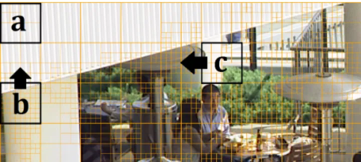
When a new CU has to be processed by the encoder, the first step is the estimation of three major indicators, based on direct neighborhood. These three indicators are: the most probable residual size, the most probable ρ-Domain slope, the most probable depth and the most probable λ. In Figure 3, we can observe several cases for CTU based prediction. Deriva-tion of these indicators is only performed from neighbor’s value. If left neighbor is available, it is used for reference (c), otherwise the above CTU is used (b). Regarding the first CTU, we use predetermined initial values (a). If a CTU has no indicators due to a lack of residual, we assign the last valid measure.
This way, we estimate for the current CTU: the residual size N , the ρ-Domain slope θ and the depth D. After com-puting these indicators and retrieving targeted bitrate R, the first step is the ρ computation, with Equation 6.
ρ = 1− R θest
(6)
Fig. 3: Different possible prediction configurations, a⇒ no predictor, b⇒ above CTU, c ⇒ left CTU.
Once ρ is available, it can be combined with the most proba-ble λ to obtain the dead-zone boundary, derived from Equa-tion 4:
DZB =−1
λ∗ log(1 − ρ) (7)
The final step consists in computing the quantization param-eter which allows to reach this DZB on residuals. The HEVC standard specification gives the following Equation for scal-ing process:
D[x][y] =T [x][y]∗ S[x][y] ∗ L[QP %6] ∗ 2 QP /6
2bdShif t +
1 2 (8) With (x,y) the coefficient position in the residual, T[x][y] the scaled coefficient, D[x][y] the transformed coefficient, S[x][y] a scaling factor (equal to 16 if no scaling list is used), bdShift described in Equation 9 and a scaling factor L[k] =
{40,45,51,57,64,72} for k=0 to 5. All these parameters are
defined in the HEVC specifications.
bdShif t = BitDepth + Log2(N )− 5 (9) When D[x][y]=DZB is reached, T[x][y]=1. Assuming that we use a 8-bit depth, without using a scaling list, we have:
F (QP ) = ( DZB−1 2 ) ∗ 2Log2(N )−1 (10) With: F (QP ) = L[QP %6]∗ 2QP /6 (11) The function F has to be inverted to get the appropriate QP. In Figure 4, we plot this function for QP = 1 to 51. To make the inversion easier, we choose to approximate this function as F (QP ) = 40∗ 2QP /6. This way, the chosen QP is slightly
increased and produces a lower bitrate. Hence, we can com-pute the appropriate QP as:
QP = 6∗ Log2 ( 1 40∗ ( DZB−1 2 ) ∗ 2Log2(N )−1 ) (12) We also hold the QP value in the interval described in Equa-tion 13, with ∆QP = 5.
Fig. 4: F(QP) function and its envelope.
3.4. Summarized Algorithm
First of all, encoding parameters are derived from neighbor-hood as described in Section 3.2. Then, the related targeted
ρ is computed as well as the dead-zone boundary, based on
Equation 6 and 7. Lastly, the quantization parameter is com-puted with Equation 12 by fulfilling the interval described in Equation 13. In order to have feedback for the next CTU en-coding, we collect the parameters described in Section 3.1.
4. EXPERIMENTAL RESULTS 4.1. Configuration
In order to check the algorithm, we have implemented it in the HM 13.0 Reference Software [5]. In Figure 5, we can observe the experimental procedure we have used. The configuration used for both encoders is the Random-Access (RA) configu-ration. This configuration is based on a succession of hier-archical structures called group of pictures (GOP). In a RA stream, pictures called random access points (RAP) appear periodically in order to clean dependencies on previously en-coded frames. In RA configuration, a base QP is defined, and a fixed δQP is added to encode a frame. The value of δQP de-pends on the frame hierarchy in the GOP and does not change while encoding. This way, the same QP is used in frames sharing the same GOP hierarchy. In our procedure, a video input feeds the two encoders. The Reference encoder com-presses the video sequence following the RA configuration. After each CTU encoding, the bitrate produced is measured and sent to the customized encoder. The customized encoder receives a targeted bitrate from the reference encoder for each CTU. Then, the algorithm described in Section 3 is performed and the chosen QP is used for CTU encoding.
We have selected the Class A test sequences for measure-ment. Class A contains five different sequences with differ-ent frame rates, and contdiffer-ents, but with the same resolution (1920x1080p). These sequences are detailed in [13]. This choice is justified by our use-case target which is high defini-tion content for broadcasting environment.
The quantization parameters used to generate bit targets are 22, 27, 32 and 37. For each sequence, all frames are en-coded and in order to compare results, we measure achieved bitrates and PSNR on all frames excepting RAP, since the Laplacian model is only defined for inter residuals.
Fig. 5: Experimental procedure. The reference encoder feeds our customized encoder with the targeted bitrate per CTU.
4.2. Results
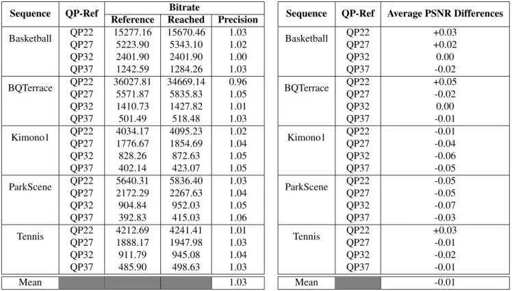
The bitrate results are reported in Table 1. In Column 2, the base QP for RA encoding is defined, and the resulting bitrate is printed in Column 3. In Column 4, the reached bitrate is displayed. The related accuracy Reached/Ref erence is computed and placed in Column 4. We can notice that the average 103% accuracy is satisfying considering the approx-imations and choices made. There is a slight bitrate over-load since there is not any correction while encoding. This is not an issue since the aim of the proposed algorithm is only to estimate the QP. The budget management will be stud-ied in our future work, as a complementary algorithm. Re-garding visual quality, we may expect an improvement of PSNR, since the bitrate tends to increase. However, we can notice in Table 2 that the proposed algorithm does not change PSNR with a -0.01dB average difference. This unexpected behaviour is explained by the fact that several syntax ele-ments (cu qp delta abs and cu qp delta sign flag) are added in order to signal the QP variations among CTUs. This extra signalisation increases the bitrate without increasing quality.
5. CONCLUSION
In this paper, we propose an innovative QP estimation scheme for the HEVC standard, with reduced complexity. The re-sults show a satisfaying bitrate error of 3% without correc-tion, and no PSNR deterioration. Our future work will aim at linking this CTU-based approach with a CTU bit allocation algorithm, in order to make a complete low complexity rate control algorithm for the HEVC standard.
REFERENCES
[1] Rec. ITU-T H.265, High Efficicency Video Coding, http://www.itu.int/rec/T-REC-H.265-201304-I.
Sequence QP-Ref Bitrate
Reference Reached Precision Basketball QP22 15277.16 15670.46 1.03 QP27 5223.90 5343.10 1.02 QP32 2401.90 2401.90 1.00 QP37 1242.59 1284.26 1.03 BQTerrace QP22 36027.81 34669.14 0.96 QP27 5571.87 5835.83 1.05 QP32 1410.73 1427.82 1.01 QP37 501.49 518.48 1.03 Kimono1 QP22 4034.17 4095.23 1.02 QP27 1776.67 1854.69 1.04 QP32 828.26 872.63 1.05 QP37 402.14 423.07 1.05 ParkScene QP22 5640.31 5836.40 1.03 QP27 2172.29 2267.63 1.04 QP32 904.84 952.03 1.05 QP37 392.83 415.03 1.06 Tennis QP22 4212.69 4241.41 1.01 QP27 1888.17 1947.98 1.03 QP32 911.79 945.08 1.04 QP37 485.90 498.63 1.03 Mean 1.03
Table 1: Achieved Bitrate Precision
[2] P. Bordes, G. Clare, F. Henry, M. Raulet, and J. Vieron, “An Overview of the Emerging HEVC Standard,” in
IEEE International Symposium on Signal, Image, Video and Communications, 2012.
[3] H. Choi, J. Nam, J. Yoo, D. Sim, and I.-V. Bajic, “Rate Control based on Unified RQ Model for HEVC,” In-put Document to JCT-VC H0213, San Jose (USA), July 2012.
[4] B. Li, H. Li, and J. Zhang, “Rate Control by R-Lambda Model for HEVC,” Input Document to JCT-VC K0103, Shangai (China), October 2012.
[5] High Efficiency Video Coding (HEVC) Test Model 13, http://hevc.hhi.fraunhofer.de/svn/svn HEVCSoftware/. [6] Zhihai He and Sanjit K. Mitra, “Optimum Bit Alloca-tion and Accurate Rate Control for Video Coding via
ρ-Domain Source Modeling,” IEEE Transactions on Circuits and Systems for Video Technology, vol. 12, no.
10, October 2002.
[7] Shanshe Wang, Siwei Ma, Shiqi Wang, Debin Zao, and Wen Gao, “Quadratic ρ-Domain Based Rate Control Algorithm for HEVC,” in IEEE International
Con-ference on Acoustics, Speech, and Signal Processing,
2014.
[8] Shanshe Wang, Shiqi Wang, Debin Zhao, and Wen Gao, “Rate-GOP Based Rate Control for High
Effi-Sequence QP-Ref Average PSNR Differences Basketball QP22 +0.03 QP27 +0.02 QP32 0.00 QP37 -0.02 BQTerrace QP22 +0.05 QP27 -0.02 QP32 0.00 QP37 -0.01 Kimono1 QP22 -0.01 QP27 -0.04 QP32 -0.06 QP37 -0.05 ParkScene QP22 -0.05 QP27 -0.05 QP32 -0.07 QP37 -0.03 Tennis QP22 +0.03 QP27 -0.01 QP32 -0.02 QP37 -0.01 Mean -0.01 Table 2: PSNR Differences
ciency Video Coding,” IEEE Journal of Selected Topics
in Signal Processing, vol. 7, no. 6, December 2013.
[9] Bumshik Lee and Munchurl Kim, “Modeling Rates and Distorsions Based on a Mixture of Laplacian Distribu-tions for Inter-Predicted Residues in Quadtree Coding of HEVC,” IEEE Signal Processing Letters, vol. 18, no. 10, October 2011.
[10] Dong-Il Park, Haechul Choi, Jin soo Choi, and Jae-Con Kim, “LCU-Level Rate Control for Hierarchical Pre-diction Structure of HEVC,” in International
Confer-ence on Consumer Electronics, 2013.
[11] Junjun Si, Siwei Ma, Shiqi Wang, and Wen Gao, “Laplace Distribution Based CTU Level Rate Control For HEVC,” in IEEE Visual Communications and
Im-age Processing Conference, 2013.
[12] Il-Koo Kim, Junghye Min, Tammy Lee, Woo-Jin Han, and JeongHoon Park, “Block Partitioning Structure in the HEVC Standard,” IEEE Transactions on Circuits
and Systems for Video Technology, vol. 22, no. 12,
De-cember 2012.
[13] T. Suzuki, R. Cohen, T.-K. Tan, and S. Wenger, “Test Sequence Material (AHG22),” Input Document to JCT-VC O0022, Geneva (Switzerland), November 2013.