HAL Id: hal-03207037
https://hal.inria.fr/hal-03207037
Submitted on 23 Apr 2021HAL is a multi-disciplinary open access
archive for the deposit and dissemination of sci-entific research documents, whether they are pub-lished or not. The documents may come from teaching and research institutions in France or abroad, or from public or private research centers.
L’archive ouverte pluridisciplinaire HAL, est destinée au dépôt et à la diffusion de documents scientifiques de niveau recherche, publiés ou non, émanant des établissements d’enseignement et de recherche français ou étrangers, des laboratoires publics ou privés.
Combining Data Assimilation and Machine Learning to
build data-driven models for unknown long time
dynamics - Applications in cardiovascular modeling
Francesco Regazzoni, Dominique Chapelle, Philippe Moireau
To cite this version:
Francesco Regazzoni, Dominique Chapelle, Philippe Moireau. Combining Data Assimilation and Machine Learning to build data-driven models for unknown long time dynamics - Applications in cardiovascular modeling. International Journal for Numerical Methods in Biomedical Engineering, John Wiley and Sons, inPress, �10.1002/cnm.3471�. �hal-03207037�
DOI: xxx/xxxx
RESEARCH ARTICLE - FUNDAMENTAL
Combining Data Assimilation and Machine Learning to build
data-driven models for unknown long time dynamics –
Applications in cardiovascular modeling
Francesco Regazzoni*
1,2,3| Dominique Chapelle
2,3| Philippe Moireau
2,31MOX - Mathematics Dept., Politecnico di
Milano, Italy
2Inria, France
3LMS, Ecole Polytechnique, CNRS, Institut
Polytechnique de Paris, France Correspondence
*Corresponding author. Email: [email protected]
Summary
We propose a method to discover differential equations describing the long-term dynamics of phenomena featuring a multiscale behavior in time, starting from measurements taken at the fast-scale. Our methodology is based on a synergetic combination of Data Assimilation (DA), used to estimate the parameters associated with the known fast-scale dynamics, and Machine Learning (ML), used to infer the laws underlying the slow-scale dynamics. Specifically, by exploiting the scale sep-aration between the fast and the slow dynamics, we propose a decoupling of time scales that allows to drastically lower the computational burden. Then, we propose a ML algorithm that learns a parametric mathematical model from a collection of time series coming from the phenomenon to be modeled. Moreover, we study the interpretability of the data-driven models obtained within the black-box learning framework proposed in this paper. In particular, we show that every model can be rewritten in infinitely many different equivalent ways, thus making intrinsically ill-posed the problem of learning a parametric differential equation starting from time series. Hence, we propose a strategy that allows to select a unique representative model in each equivalence class, thus enhancing the interpretability of the results. We demonstrate the effectiveness and noise-robustness of the proposed methods through several test cases, in which we reconstruct several differential models starting from time series generated through the models themselves. Finally, we show the results obtained for a test case in the cardiovascular modeling context, which sheds light on a promising field of application of the proposed methods.
KEYWORDS:
Machine Learning, Data Assimilation, Artificial Neural Networks, Data-driven Modeling, Multiscale Problems, Cardiovascular Modeling
1
INTRODUCTION
Mathematical models are built upon two types of sources, namely a priori information (physics principles, simplifying assump-tions, empirical laws, etc.) and experimental data. The relative weight of the two sources should be properly balanced: the fewer data are available, the stronger a priori assumptions are needed. By moving towards the Big Data era, mathematical models are
fed with more and more data, reducing the necessity of strong a priori assumptions. The asymptote of this process is data-driven
modeling, that is to say the construction of a mathematical model for a given phenomenon solely on the basis of experimental
data, as opposed to physics-based modeling, that on the other hand makes use of data only to tune the parameters appearing in equations written on the basis of a detailed study of the phenomenon by the modeler. Between pure physics or pure data, hybrid approaches allow to circumvent the uncertainties inherent to physics-based models by making full use of the data available on the system. This is particularly the case when developing estimation strategies of dynamical models1,2, with a particular concern in identification - i.e. parameter estimation - of such systems3,4,5,6. Note that these strategies are also known as Data Assimilation (DA) approaches in the engineering community since their introduction in environmental sciences in the late 70s7.
Data-driven modeling appears particularly advantageous when traditional modeling encounters limitations. A representative case is given by systems whose behavior is well understood and accurately modeled, but for which the model parameters them-selves feature a long-term evolution that is difficult to predict because the underlying mechanisms are not fully elucidated. This motivates the idea of resorting to a data-driven approach to apprehend the slow-scale parameter evolution, while still relying on the mathematical model at the fast scale. This is the specific focus of this paper. Examples are given by the long-term remodel-ing of biological systems and by the development of diseases under the influence of factors such as lifestyle or environmental conditions that are hardly within reach of mathematical modeling. In Sec. 1.3 we consider an example model inspired by the development of hypertension.
Data-driven modeling poses the problem of finding the laws governing the evolution of a given phenomenon (a natural phe-nomenon, an engineering process, a system of agents, etc.) starting from its observation. Here comes the challenge of leveraging the information contained in large amounts of data to extract knowledge, by finding the principles hidden in data.
In the past few years, several algorithms have been proposed to automate the process – historically a human prerogative – of discovering the laws hidden in experimental data. In this paper we consider data-driven modeling of time-dependent phenomena. With respect to most Machine Learning (ML) techniques that are designed to learn the steady-state relationship between two quantities, the introduction of the time variable dramatically increases the complexity of the problem since the object to be learned is not a function, but, typically, a differential equation.
1.1
Learning time-dependent models from data
Data-driven algorithms capable of building black-box time-dependent models have been developed with the two following goals: • Data-driven modeling: in this case data come from experimental measurements of a given phenomenon that one wants to
understand and possibly predict (this is the case considered in this paper);
• Data-driven model order reduction (MOR): in this case data are generated by an high-fidelity model and the goal is to obtain a different model (hopefully with fewer variables and with a lower computational complexity) reproducing – up to some error – the same input-output map8,9,10,11.
In most cases, the algorithms developed for one goal are also suited for the other one. Hence, in this section, we review the algorithms proposed in the literature for either goal.
Symbolic regression12,13,14is a technique to find a model, written as a differential equation in symbolic form, by means of an iterative process consisting in the generation of candidate symbolic differential equations and in the selection of the best ones.
In15the authors propose a data-driven MOR technique for systems with linear state dependence, based on the idea of inferring the frequency-domain response of the linear system from a collection of trajectories and to apply the Loewner framework16to interpolate the transfer function measurements at a collection of interpolation points.
Sparse Identification of Nonlinear Dynamics (SINDy, see17) is an algorithm that infers a dynamical system from a collection of measurements on the system – the state, the time derivative of the state and the input at different times – under the assumption that the right-hand side of the model depends on a few combination of predetermined functions of the input and the state (linear combinations, products and trigonometric functions). In18 a similar ML technique is employed to predict metabolic pathway dynamics from time series multiomics data. In19a nonlinear differential equation is learned from data, by assuming a polynomial form with sparse coefficients by compressive sensing. In20the authors proposed a method to infer an ODE (Ordinary Differential Equation) representation of a model from time-dependent output data. The right-hand side of the ODE is represented as a linear combination of multivariate polynomials of (at most) quadratic order in each state variable.
In21 an S-system (a class of models inspired by the mass-action kinetics) is trained by Bayesian model selection to learn a time-dependent dynamics.
Dynamic Mapping Kriging (DMK, see22) is an extension to the time-dependent case of Kriging23or Gaussian Process (GP) regression24,25. Kriging is a regression method that uses a GP, with a covariance function dependent on hyper-parameters to be tuned from data, as prior for the outcome of a function. DMK consists in performing Kriging on a difference equation, where the independent variables are the state and the input of a system at the current time step, and the dependent variable is the state at the next time step.
In26a technique based on Artificial Neural Networks (ANNs) to learn a time-dependent differential equation from a collection of input-output pairs has been proposed. The authors also provided a universal approximation result stating that these ANN models can approximate any time-dependent model with arbitrary accuracy. In27this method has been extended by informing the learning machine with some a priori knowledge on the system to learn, moving from a purely black-box framework to a semi-physical (or grey-box) one. A similar ANN model is proposed in28, where an efficient algorithm for sensitivities computation is discussed.
Learning algorithms for data-driven discovery of PDEs, either based on ANNs (see e.g.29,30,31) or GP32,33have been proposed. Those methods require the knowledge of the form of the equations and are thus better suited for the identification of parameters. In34the authors proposed an ANN-based algorithm to discover nonlinear time-dependent models from a collection of snapshots of the state of the system, by minimizing the residual of some given multi-step time-stepping scheme. In35the authors proposed an ANN-based method to build a surrogate model, using the physical knowledge as a constraint. In36the method of31has been applied to the identification of the constitutive relationship underlying a PDE, starting from snapshots of the solution.
1.2
Accounting for inter-individual variability
The above mentioned methods seek a unique model capable of describing the evolution of some quantities, based on a training set composed of observed trajectories. In many applications, however, each trajectory is referred to a different individual of some group (e.g. human beings). Since each individual is different, one should thus look for a family of models, rather than a unique model; or, from another perspective, for a single model dependent on some parameters, accounting for inter-individual variability.
Whereas parametric models are widely used in traditional physics-based modeling, the introduction of parameters raises conceptual difficulties when dealing with data-driven modeling since, in a black-box framework, parameters cannot be measured. Moreover, assuming that the learning algorithm is capable of assigning to each training individual a parameter value, then the problem of interpretability comes into play. What is the physical meaning of such learned parameters? The lack of interpretability also hampers the use of the learned models for predictive purposes since, without a clear physical meaning of the parameters, one cannot easily determine the parameters associated with an individual not included in the training set.
In this paper we show how a wise interplay between ML and DA techniques can help to deal with those issues. We define in such a way a framework to perform data-driven modeling of phenomena featuring inter-individual variability, without renouncing to interpretability and predictivity of the learned model.
1.3
A motivating example: arterial network remodeling
To motivate the approach and to help fix the ideas with the notation, we provide in this section an example that can be treated with the framework proposed in this paper. In Sec. 3.4 we consider again this example, by showing some numerical results. Specifically, we consider the slow development of diseases related to the remodeling of the arterial network (such as hyper-tension). Even if the dynamics at the fast scale (order of seconds) of the circulation of blood through the network has been deeply studied and relatively well understood (different mathematical models, from lumped-parameters models37 to complex three-dimensional fluid-structure interaction models38,39are available), the mechanisms driving the long-term evolution of the arterial network are not fully elucidated. Indeed, in spite of some important steps towards the understanding of the determinants of vascular remodeling40,41, a comprehensive mathematical model capable of predicting the development and evolution of this phenomenon is still missing.
FIGURE 1Visual representation of the two-stage Windkessel model of Eq. (1). In this electrical analogy, current represents
blood flux, while voltage represents blood pressure. The heart is represented as a current generator, while the arterial network comprises dissipative and compliant elements, represented by resistances and capacitors, respectively.
For the sake of simplicity, we consider a simple model to describe the evolution in the fast-scale dynamics, namely the two-stage Windkessel model (see Fig. 1), which reads37
⎧ ⎪ ⎪ ⎪ ⎪ ⎨ ⎪ ⎪ ⎪ ⎪ ⎩ d d𝑡𝑃p(𝑡) = 𝑃d(𝑡) − 𝑃p(𝑡) 𝑅p𝐶p + 𝑄(𝑡) 𝐶p 𝑡∈ (0, 𝑇 ], d d𝑡𝑃d(𝑡) = 𝑃p(𝑡) − 𝑃d(𝑡) 𝑅p𝐶d + 𝑃vs− 𝑃d(𝑡) 𝑅d𝐶d 𝑡∈ (0, 𝑇 ], 𝑃p(0) = 𝑃p,0, 𝑃d(0) = 𝑃d,0, (1)
where we denote by 𝑥(𝑡) = (𝑃p(𝑡), 𝑃d(𝑡))the state of the model, given by the proximal and distal pressures; we denote the parameters of the fast-scale model by 𝜃 = (𝑅p, 𝐶p, 𝑅d, 𝐶d), respectively the proximal and distal resistance and compliance; 𝑄(𝑡) is the blood flux. We suppose then to be able to measure the proximal pressure at a collection of time instants (𝑡1,… , 𝑡𝐾)and we collect all the measurements into the observation vector 𝑧 = (𝑃p(𝑡1), … , 𝑃p(𝑡𝐾)).
When considering the fast time scale (i.e. the typical time scale of a heartbeat), the value of 𝜃, describing the properties of the arterial network, is fixed. However, if we consider a longer time scale (days and above), 𝜃 may evolve, possibly associated with some disease. For instance, hypertension is linked to an increase of the arterial resistance 𝑅𝑑, which requires a higher systolic pressure to preserve the cardiac output. We thus introduce a slow time variable 𝜏 and we write 𝜃(𝜏), assuming that the fast-scale parameters are in fact functions of the slow-scale time variable.
We consider the following scenario. Suppose that we have a set of 𝑁𝑃 patients, periodically monitored over the long-term horizon at times (𝜏1 < 𝜏2 < ⋯ < 𝜏𝑁𝑆). At each time 𝜏𝑗 (for 𝑗 = 1, … , 𝑁𝑆), the arterial pressure of the 𝑖-th patient (for
𝑖 = 1, … , 𝑁𝑃) is measured for a few seconds, collecting the observation vector 𝑧 𝑖
𝑗. More precisely, we denote the measured observation vector by ̃𝑧𝑖 𝑗= 𝑧 𝑖 𝑗+ 𝜒 𝑖 𝑗, where 𝜒 𝑖
𝑗is the measurement error. The measurement ̃𝑧 𝑖
𝑗reflects the value of the fast-scale parameters of the 𝑖-th patient at the slow-scale time 𝜏𝑗, which we define as 𝜃
𝑖 𝑗 ∶= 𝜃
𝑖(𝜏
𝑗), where 𝜃𝑖(𝜏)denotes the slowly evolving
𝑖-th patient’s parameters of the fast-scale model.
The goal is to learn a model for the slow-scale evolution of 𝜃(𝜏) from the collection of noisy measurements {̃𝑧𝑖 𝑗}
𝑖=1,…,𝑁𝑃 𝑗=1,…,𝑁𝑆. As
mentioned before, all patients are different, and thus inter-individual variability must be taken into account.
1.4
Paper outline
The paper is organized as follows. In Sec. 2, we state in mathematical terms the problem that we deal with in this paper and we introduce the associated notation. Then, we present the methods that we propose to solve such a problem, based on a decoupling of the time scales. In Sec. 3, we show the effectiveness and the noise-robustness of the proposed methods by means of several numerical test cases. Finally, in Sec. 4, we critically discuss the results obtained and we draw our conclusions.
2
PROBLEM STATEMENT AND PROPOSED METHODS
In this section, motivated by the example of Sec. 1.3, we state the setting of the problem that we consider in this paper, in which the example of Sec. 1.3 can be recast, before introducing and analysing our proposed methods.
We consider a collection of 𝑁𝑃 individuals, such that the 𝑖-th individual is associated with 𝜃𝑖(𝜏) ∈ ⊂ ℝ𝑁𝜃, which evolves with a slow dynamics driven by an equation of the form
⎧ ⎪ ⎨ ⎪ ⎩ d d𝜏𝜃 𝑖 (𝜏) = 𝑔(𝜃𝑖(𝜏), 𝛼𝑖) 𝜏∈ (0,T], 𝜃𝑖(0) = 𝜃𝑖 0, (2) where 𝛼𝑖 ∈ A ⊂ ℝ𝑁𝛼 are parameters characterizing the 𝑖-th individual at the slow-scale, accounting for inter-individual
variability. In this paper, we always assume that
𝑔∈ ∶= {𝑔 ∈ 0(ℝ𝑁𝜃×𝑁𝛼; ℝ𝑁𝜃), Lipschitz continuous in 𝜃},
so that the models admit a unique solution for each initial state and parameter.
This slow-scale model is coupled with a fast-scale dynamics, for which 𝜃𝑖(𝜏)can be considered as a constant. Specifically, we consider a collection of times (𝜏1 < 𝜏2 <⋯ < 𝜏𝑁𝑆)over the long-term horizon, and we write 𝜃
𝑖 𝑗 ∶= 𝜃
𝑖(𝜏
𝑗), for 𝑗 = 1, … , 𝑁𝑆 and 𝑖 = 1, … , 𝑁𝑃. We consider a model for the fast-scale dynamics with the following form
⎧ ⎪ ⎨ ⎪ ⎩ d d𝑡𝑥 𝑖 𝑗(𝑡) = 𝑓 (𝑥 𝑖 𝑗(𝑡), 𝜃 𝑖 𝑗, 𝑡) 𝑡∈ (0, 𝑇 ), 𝑥𝑖 𝑗(0) = 𝑥 𝑖 𝑗,0, (3) where 𝑥𝑖 𝑗(𝑡) ∈ ⊂ ℝ
𝑁𝑥 is the fast-scale state. We recall that 𝜃𝑖
𝑗 are considered as constant parameters at this scale (we assume
𝑇 ≪ 𝜏𝑗− 𝜏𝑗−1). On this system, we consider an observation process given at the fast scale, namely
𝑧𝑖𝑗= 𝑇 ∫ 0 ℎ(𝑥𝑖𝑗, 𝑡) d𝑡, (4) where 𝑧𝑖 𝑗 ∈ ⊂ ℝ
𝑁𝑧and we define the measured observations as ̃𝑧𝑖 𝑗 = 𝑧 𝑖 𝑗+ 𝜒 𝑖 𝑗, where 𝜒 𝑖
𝑗 ∼ (0, 𝑊 ) are the measurement errors that we assume to be i.i.d. and Gaussian with covariance matrix 𝑊 . In the example of Sec. 1.3, the observation vector contains direct measurements of the first entry of the state 𝑥 at a collection of discrete times 𝑡𝑘, for 𝑘 = 1, … , 𝐾. This can be written in the form of Eq. (4) by defining the observation map as ℎ(𝑥, 𝑡) ∶= ∑𝐾
𝑘=1𝑥⋅ 𝑒1𝛿(𝑡 − 𝑡𝑘) 𝑒𝑘, where 𝑒𝑘denotes the 𝑘-th element of 𝑘-the canonical basis of ℝ𝑛and where 𝛿 denotes the Dirac delta function (in fact, given a function 𝑓(𝑡), we have ∫0𝑇𝑓(𝑡)𝛿(𝑡 − 𝑡𝑘) d𝑡 = 𝑓 (𝑡𝑘)).
We assume that we have perfect knowledge about the equation driving the fast-scale evolution and that we want to identify a model to describe the slow-scale evolution. Specifically, we assume that we know:
(K1) 𝑓, ℎ: the fast-scale evolution and observation laws; (K2) {̃𝑧𝑖
𝑗} 𝑖=1,…,𝑁𝑃
𝑗=1,…,𝑁𝑆: the fast-scale measurements;
whereas we do not know:
(U1) 𝑔: the slow-scale evolution law;
(U2) {𝛼𝑖}𝑖=1,…,𝑁𝑃: the slow-scale parameters of individuals;
(U3) {𝜃𝑖 0}
𝑖=1,…,𝑁𝑃: the slow-scale initial states of individuals, for which we assume a prior distribution ( ̄𝜃, 𝛱 𝜃); (U4) {𝑥𝑖
𝑗,0} 𝑖=1,…,𝑁𝑃
𝑗=1,…,𝑁𝑆: the fast-scale initial states of individuals, for which we assume a prior distribution ( ̄𝑥, 𝛱𝑥).
The goal is to identify the unknown objects (U1)–(U4) from the known ones (K1)–(K2). We notice that this task is situated in an intermediate position between the fields of DA, as we here seek to identify the parameters and the state for a known dynamics, and ML, as we seek to discover the law driving the slow-scale (unknown) dynamics. We remark that the setting considered in this paper differs from that of a standard parameters identification problem, in which one aims to identify unknown parameters
of a known model from time series data (see e.g.3,4,42), for two main reasons. First, the observations ̃𝑧𝑖
𝑗are taken at the fast-scale, while we are interested in inferring knowledge at the slow-scale. Secondly, we assume that we are agnostic of the model whose parameters we aim to identify. As a matter of fact, we aim at simultaneously learning the parameters 𝛼𝑖 and the differential equation (2).
2.1
General strategy
In this paper we propose to combine ML and DA concepts in order to address the problem presented above. Specifically, con-cerning the task of learning the law 𝑔 given the measurements {̃𝑧𝑖
𝑗} 𝑖=1,…,𝑁𝑃
𝑗=1,…,𝑁𝑆, we extend the strategy proposed in
26. Hence, we select a set of candidate laws 𝑛 (where 𝑛 indicates that the set is parametrized by a finite number of parameters), such that 𝑛 ⊂ , and we look for the model, inside the family 𝑛, that best fits the available data. This can be interpreted, by assum-ing Gaussian distribution of the measurement errors, as the maximum-likelihood estimation of the evolution law 𝑔 inside the family 𝑛. This formalism allows to write the problem of identifying/learning the objects (U1)–(U4) in a unified minimization framework, as we show in the next section.
2.1.1
A unified minimization framework
The maximum likelihood estimation of the unknown objects is found by minimizing the negative log-likelihood ( ̂ 𝑔,{̂𝛼𝑖}𝑖,{̂𝜃0𝑖}𝑖,{̂𝑥𝑖𝑗,0}𝑖𝑗)= argmin 𝑔∈𝑛 {𝛼𝑖}𝑖∈A𝑁𝑃 {𝜃𝑖 0} 𝑖∈𝑁𝑃 {𝑥𝑖 𝑗,0} 𝑖 𝑗∈𝑁𝑃 𝑁𝑆 𝑁𝑃 ∑ 𝑖=1 (∑𝑁𝑆 𝑗=1 (1 2|𝑧 𝑖 𝑗− ̃𝑧 𝑖 𝑗| 2 𝑊−1+ 1 2|𝑥 𝑖 𝑗,0− ̄𝑥| 2 𝛱−1 𝑥 ) +1 2|𝜃 𝑖 0− ̄𝜃| 2 𝛱−1 𝜃 ) , (5) such that (2), (3) and (4) hold true. Here and in what follows, given a vector 𝑤 ∈ ℝ𝑛and a symmetric positive-definite matrix
𝑄∈ ℝ𝑛×𝑛, we denote by |𝑤|
𝑄 ∶= (𝑤𝑇𝑄𝑤)1∕2the energy norm. Moreover, for the sake of brevity, we denote by {⋅} 𝑖 𝑗and {⋅}
𝑖 sets indexed by 𝑗 = 1, … , 𝑁𝑆and 𝑖 = 1, … , 𝑁𝑃, where the values taken by the indexes 𝑗 and 𝑖 are left implicit.
Problem (5) can be interpreted as that of finding the slow-scale law, the slow-scale parameter for each individual, and the initial state at both scales such that the resulting outputs 𝑧𝑖
𝑗best approximate the measured outputs ̃𝑧 𝑖
𝑗. The last two terms of the loss functional can be regarded as regularization terms.
2.1.2
Decoupling the two scales
Despite its solid foundation, the solution of Problem (5) may be unaffordable in practice, because of the huge number of differ-ential equations that serve as constraints for the minimization problem. Indeed, Problem (5) is constrained by the 𝑁𝑃 slow-scale differential equations (2) and the 𝑁𝑃× 𝑁𝑆differential equations (3). Moreover, Problem (5) attempts to simultaneously identify objects related to both the slow scale and the fast scale for each 𝑗 = 1, … , 𝑁𝑆and 𝑖 = 1, … , 𝑁𝑃.
To lower the complexity of Problem (5), we propose to exploit the scale separation between the fast and the slow dynamics, and to split the problem into two steps:
(P1) The first step consists in finding an estimate for 𝜃𝑖
𝑗, for each 𝑗 = 1, … , 𝑁𝑆 and 𝑖 = 1, … , 𝑁𝑃, on the basis of the measurements ̃𝑧𝑖
𝑗, by solving the problem ( ̂ 𝜃𝑖𝑗, ̂𝑥𝑖𝑗,0 ) = argmin 𝜃𝑖 𝑗∈ 𝑥𝑖 𝑗,0∈ (1 2|𝑧 𝑖 𝑗− ̃𝑧 𝑖 𝑗| 2 𝑊−1+ 1 2|𝑥 𝑖 𝑗,0− ̄𝑥| 2 𝛱−1 𝑥 + 1 2|𝜃 𝑖 𝑗− ̄𝜃| 2 𝛱−1 𝜃 ) , (6) such that (3) and (4) hold true.
(P2) Once the estimates {̂𝜃𝑖 𝑗}
𝑖=1,…,𝑁𝑃
𝑗=1,…,𝑁𝑆are available, we consider the problem
( ̂ 𝑔,{̂𝛼𝑖}𝑖,{̂𝜃𝑖 0} 𝑖)= argmin 𝑔∈𝑛 {𝛼𝑖}𝑖∈A𝑁𝑃 {𝜃𝑖 0} 𝑖∈𝑁𝑃 𝑁𝑃 ∑ 𝑖=1 𝑁𝑆 ∑ 𝑗=1 1 2|𝜃 𝑖(𝜏 𝑗) − ̂𝜃𝑗𝑖| 2 𝛱−1 𝜃 , (7) such that (2) holds true.
We notice that (P1) involves only the fast-scale dynamics, whereas (P2) only the slow-dynamics. Indeed, the two scales have been decoupled. As a consequence, in (P1), each individual and each slow-scale instant 𝜏𝑗can be treated separately; the problem can be solved for each 𝑗 = 1, … , 𝑁𝑆and 𝑖 = 1, … , 𝑁𝑃 independently of each other. This allows for a possibly parallel solution of (P1). Moreover, differently from Problem (5), in Problems (P1) and (P2) objects related to the fast and slow scales are never simultaneously identified. In other words, the complex Problem (5) has been split into (𝑁𝑃𝑁𝑆+ 1)simpler problems.
A further effect of splitting Problem (5) into two steps, is that Problems (P1) and (P2) feature different natures. While the former is a purely DA problem, as it consists in the identification of the state and the parameters for System (3), the latter is a learning problem, as the laws governing the slow-scale dynamics need to be discovered. This is a consequence of the decoupling between the fast-scale, driven by a known dynamics, from the slow-scale, whose dynamics is governed by unknown laws.
Several identifications procedures are available in the literature for the solution of problems written in the form of (P1) (see e.g.3,4,5,6). In this paper, we restrict our scope to measurements sampled in time, instead of continuous signals, and we consider a state and parameter sequential estimation strategy43,2,6based on the extended Kalman filter (EKF), an extension of the Kalman filter (KF) algorithm to nonlinear systems, performed at each step, of Eq. (3)43,7. We recall that whereas KF is equivalent to least square estimation for linear dynamics, EKF only gives an approximation of the least square estimation (P1) with, however, the benefit of being “on the fly”. This is particularly adapted to the fast-scale dynamics where we can typically face real-time monitoring constraints.
2.1.3
Interpretation of the learned model
Before presenting an algorithm for the solution of Problem (P2) (which is treated in Sec. 2.2), we deal with the problem of interpreting the solution of Problem (P2) itself. This is instrumental to the presentation of the proposed methods. Therefore, in this section we assume the existence of an algorithm capable of solving Problem (P2) and we speculate about the interpretation of its solution. Solving Problem (P2) serves indeed different purposes, which we list in what follows.
Understanding.
First, the function ̂𝑔 provides insight into the phenomenon under exam. Indeed, ̂𝑔 yields a description of the underlying laws written in mathematical terms and as such it can provide understanding of the phenomenology. Moreover, an analysis of the features of the function ̂𝑔 may reveal properties such as states of equilibrium, symmetry properties and relationships among the variables that may not be immediatly identifiable from the observation of the experimental data.
Classification of training individuals.
By solving Problem (P2), a (possibly vector-valued) parameter ̂𝛼𝑖is assigned to each individual. However, the physical meaning of such parameters is not clear, as they are learned in a black-box manner. Moreover, the value of such parameters in the solution of Problem (P2) is not unique: given a solution of Problem (P2), one can always find an equivalent solution with different values of the parameters (we will deal extensively with this issue in Sec. 2.3).
Nonetheless, even if we cannot interpret such parameters in physical terms, we know that they characterize the variability among the individuals. Indeed, one may be tempted to conclude that similar parameters reveal similarities among individuals (that is to say, if ̂𝛼𝑖 ≃ ̂𝛼𝑘, then the 𝑖-th and the 𝑘-th individuals are similar). In Sec. 2.3 we will show under which conditions this conclusion is licit. In that case, the learned parameters {̂𝛼𝑖}𝑖allow to classify the individuals.
For instance, in the example of Sec. 1.3, the parameter 𝛼 may describe how the arterial network of a given patient remodels in time, and thus it can be regarded as an indication of the severity of related pathologies.
Predictions.
The ultimate aim of mathematical models is making predictions. However, the lack of physical meaning of the parameter 𝛼 apparently undermines this possibility for the learned model ̂𝑔. In fact, let us consider a new individual (i.e. not employed to train the model), which we denote as the (𝑁𝑃 + 1)-th individual; to solve Problem (P2) with the learned model ̂𝑔, in order to predict the evolution of 𝜃𝑁𝑃+1(𝜏), one needs to know 𝛼𝑁𝑃+1. However, unlike the parameters of physics-based models that, having a
physical meaning, can be measured in practice, the parameters of data-driven models cannot be measured.
This inconvenience can be overcome by combining once again ML with DA (the latter acting this time at the slow-scale). All we need is to observe the (𝑁𝑃 + 1)-th individual for a (short) interval of time, on the slow-scale, 𝜏 ∈ [0,Tobs], with
Tobs<T. During this observation time interval, we collect the observations ̃𝑧𝑁𝑃+1
𝑗 , associated with the slow-scale time instants 0 = 𝜏1 < 𝜏2 < … 𝜏𝑁obs𝑆 = Tobs, and we find the estimates, by solving (P1), for the associated fast-scale parameters ̂𝜃
𝑁𝑃+1 𝑗 .
Then, by the slow-scale evolution of such parameters, we estimate the value of ̂𝛼𝑁𝑃+1, by solving the following DA problem ( ̂ 𝛼𝑁𝑃+1, ̂𝜃𝑁𝑃+1 0 ) = argmin 𝛼𝑁𝑃 +1∈A 𝜃𝑁𝑃 +10 ∈ (𝑁𝑆obs ∑ 𝑗=1 1 2|𝜃 𝑁𝑃+1(𝜏 𝑗) − ̂𝜃 𝑁𝑃+1 𝑗 | 2 𝑈−1+ 1 2|𝜃 𝑁𝑃+1 0 − ̄𝜃| 2 𝛱−1 𝜃 + 1 2|𝛼 𝑁𝑃+1− ̄𝛼|2 𝛱−1 𝛼 ) , (8)
subject to the constraint
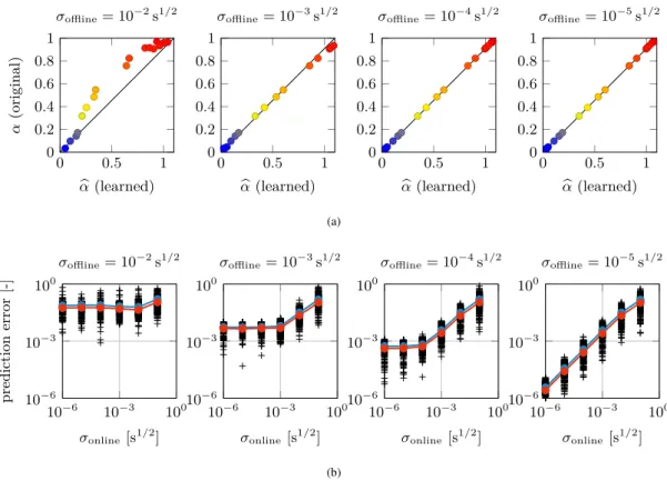
⎧ ⎪ ⎨ ⎪ ⎩ d d𝜏𝜃 𝑁𝑃+1(𝜏) = ̂𝑔(𝜃𝑁𝑃+1(𝜏), 𝛼𝑁𝑃+1), 𝜏∈ (0,Tobs] 𝜃𝑁𝑃+1(0) = 𝜃𝑁𝑃+1 0 . (9) In Eq. (8), 𝑈 denotes the covariance matrix associated with the error introduced during the resolution of the DA Problem (P1). We remark that 𝑈 can be estimated whenever Problem (P1) is solved, e.g., by an algorithm of the Kalman Filter family. Alternatively, assuming that the error introduced by the DA algorithm can be considered as a white noise of magnitude 𝜎𝑑𝐵(𝜏)
𝑑𝜏 (𝐵(𝜏) being a Wiener process), we set 𝑈 = 𝜎2∕Δ𝜏 𝐼, where 𝐼 is the 𝑁
𝜃× 𝑁𝜃 identity matrix. On the other hand, ̄𝛼 and 𝛱𝛼respectively denote the expected value and the covariance matrix associated with the slow-scale parameter 𝛼, estimated from the parameters {𝛼𝑖}𝑖=1,…,𝑁𝑃 learned during the step (P2). Specifically, we set ̄𝛼 equal to the arithmetic mean of these parameters and 𝛱
𝛼equal to their sample covariance.
We can finally employ the estimated slow-scale parameter ̂𝛼𝑁𝑃+1 to predict the evolution of 𝜃𝑁𝑃+1(𝜏)in the time interval
(Tobs,T], by solving ⎧ ⎪ ⎨ ⎪ ⎩ d d𝜏 ̂ 𝜃𝑁𝑃+1(𝜏) = ̂𝑔(𝜃𝑁𝑃+1(𝜏), ̂𝛼𝑁𝑃+1), 𝜏∈ (Tobs,T] ̂ 𝜃𝑁𝑃+1(Tobs) = ̂𝜃𝑁𝑃+1 𝑁𝑆obs . (10) To summarize, in a preliminary offline phase, we learn Model (2) from the observation of a set of training individuals, by combining DA at the fast-scale with ML at the slow-scale. Then, in the online phase, we employ DA on both the fast-scale and, for a short interval, on the slow-scale [0,Tobs]to characterize the features of a new individual, so that the previously learned model can be used to predict the evolution of this individual. The interplay that takes place, at different levels, between DA and ML is summarized in Fig. 2.
2.2
Learning a differential equation from data
In this section we present an algorithm to numerically solve Problem (P2). The algorithm presented in this paper represents an extension of the algorithm presented in26, whose goal is learning a (possibly parametric) time-dependent differential equation from a collection of input-output time-series. However, in26, the parameters associated with the training data are assumed to be known, while in this paper we need to learn them simultaneously to learning the model. The backbone of the algorithm proposed in this paper is based on that presented in26. Therefore we recall here the main ideas and we highlight the differences, while we refer to26for the details common to both algorithms. The algorithm is based on a ANN-based representation of the function 𝑔, which is trained by computing sensitivities through the adjoint method44. A similar approach is presented in28under the name of Neural ODEs, in which the state equation is discretized by means of a Runge-Kutta method45. Our algorithm represents a generalization of this method to some extent, as it learns a parametric differential equation with unknown parameters, rather than assuming that all the samples share the same dynamics.
2.2.1
Solution strategy
Following26, we parametrize 𝑔 by a finite number of real parameters 𝜇 ∈ ℝ𝑛 and we define the set of candidate laws as 𝑛 = {(𝜃, 𝛼) → 𝑔(𝜃, 𝛼; 𝜇) ∶ 𝜇 ∈ ℝ𝑛}. For the moment, we do not detail how this parametrization is performed, in order to not restrict ourselves to a specific case. To fix ideas, the reader can think of 𝑔 as a polynomial in 𝜃 and 𝛼, where 𝜇 are the coefficients of the polynomial.
Slow-scale evolution
Artificial Neural Network
Training set of patients New patient
Period of observation Fas t-sc al e Slo w -sc al e Offline Online Fast-scale (physics-based) Mathematical Model ✓Classification ✓Prediction DA DA DA ML Slow-scale (data-driven) Mathematical Model
✓Understanding
FIGURE 2Interplay between ML (green arrow) and DA (blue arrows).
Problem (P2) can thus be rewritten as the following discrete constrained optimization problem ⎧ ⎪ ⎪ ⎪ ⎨ ⎪ ⎪ ⎪ ⎩ min 𝜇∈ℝ𝑛 {𝛼𝑖}𝑖∈A𝑁𝑃 {𝜃𝑖 0} 𝑖∈𝑁𝑃 𝑁𝑃 ∑ 𝑖=1 𝑁𝑆 ∑ 𝑗=1 1 2|𝜃 𝑖 (𝜏𝑗) − ̂𝜃 𝑖 𝑗| 2 𝛱−1 𝜃 s.t. d d𝜏𝜃 𝑖 (𝜏) = 𝑔(𝜃𝑖(𝜏), 𝛼𝑖; 𝜇), 𝜏∈ (0,T], 𝑖= 1, … , 𝑁𝑃 𝜃𝑖(0) = 𝜃𝑖 0, 𝑖= 1, … , 𝑁𝑃, (11) where {̂𝜃𝑖 𝑗} 𝑖=1,…,𝑁𝑃
𝑗=1,…,𝑁𝑆are given. To derive the gradient of the cost functional = ∑ 𝑁𝑃 𝑖=1 ∑𝑁𝑆 𝑗=1 1 2|𝜃 𝑖(𝜏 𝑗) − ̂𝜃𝑗𝑖| 2 𝛱−1 𝜃
under the constraint given by Eq. (2), we introduce a family of Lagrange multipliers 𝜎𝑖∈0([0,T];) and we write the Lagrangian associated with Problem (11) (𝜇,{𝛼𝑖}𝑖,{𝜃0𝑖}𝑖,{𝜃𝑖}𝑖,{𝜎𝑖}𝑖) = 𝑁𝑃 ∑ 𝑖=1 𝑁𝑆 ∑ 𝑗=1 1 2|𝜃 𝑖 (𝜏𝑗) − ̂𝜃 𝑖 𝑗| 2 𝛱−1 𝜃 − 𝑁𝑃 ∑ 𝑖=1 T ∫ 0 (d d𝜏𝜃 𝑖 (𝜏) − 𝑔(𝜃𝑖(𝜏), 𝛼𝑖; 𝜇))⋅ 𝜎𝑖(𝜏)𝑑𝜏 − 𝑁𝑃 ∑ 𝑖=1 ( 𝜃𝑖(0) − 𝜃0𝑖)⋅ 𝜎𝑖(0) = 𝑁𝑃 ∑ 𝑖=1 𝑁𝑆 ∑ 𝑗=1 1 2|𝜃 𝑖 (𝜏𝑗) − ̂𝜃 𝑖 𝑗| 2 𝛱−1 𝜃 + 𝑁𝑃 ∑ 𝑖=1 T ∫ 0 𝜃𝑖(𝜏)⋅ d d𝜏𝜎 𝑖 (𝜏)𝑑𝜏 + 𝑁𝑃 ∑ 𝑖=1 T ∫ 0 𝑔(𝜃𝑖(𝜏), 𝛼𝑖; 𝜇)⋅ 𝜎𝑖(𝜏)𝑑𝜏 − 𝑁𝑃 ∑ 𝑖=1 𝜃𝑖(T)⋅ 𝜎𝑖(T) + 𝑁𝑃 ∑ 𝑖=1 𝜃𝑖 0⋅ 𝜎 𝑖 (0),
where the last inequality is obtained by integrating by parts the time integral. By setting to zero the variation of the Lagrangian with respect to the variables {𝜃𝑖}𝑖we get the adjoint equations, valid for 𝑖 = 1, … , 𝑁
𝑃 ⎧ ⎪ ⎨ ⎪ ⎩ − d d𝜏𝜎 𝑖(𝜏) = ∇𝑇 𝜃𝑔(𝜃 𝑖(𝜏), 𝛼𝑖; 𝜇) + 𝑁𝑆 ∑ 𝑗=1 𝛱𝜃−1 ( ̂ 𝜃𝑖𝑗− 𝜃𝑖(𝜏))𝛿 𝜏𝑗(𝜏), 𝜏∈ [0,T) 𝜎𝑖(T) = 0, (12) Finally, by computing the variation of the Lagrangian with respect to the design variables we get the gradient of the cost functional with respect to the design variables themselves
∇𝜇 = 𝑁𝑃 ∑ 𝑖=1 T ∫ 0 ∇𝑇 𝜇𝑔(𝜃 𝑖(𝜏), 𝛼𝑖; 𝜇) 𝜎𝑖(𝜏)𝑑𝜏; ∇ 𝛼𝑖 = T ∫ 0 ∇𝑇 𝛼𝑔(𝜃 𝑖(𝜏), 𝛼𝑖; 𝜇) 𝜎𝑖(𝜏)𝑑𝜏; ∇ 𝜃𝑖 0 = 𝜎 𝑖(0). (13)
Given the gradient of the cost functional, any gradient-based optimization (or training) algorithm can be used to find an approx-imate solution of Problem (11). To produce the results shown in this paper, we employed the Levenberg-Marquardt algorithm (see e.g.46), which is specifically designed for least-squares problems, coupled with a line-search for the step length, as illustrated in26.
Following26, we discretize the state equations in (11) by means of the Forward Euler scheme. The choice of an explicit scheme is aimed at lowering the computational cost of the training phase. To find the discrete version of the adjoint equations (12), we write the Lagrangian associated with the fully discretized version of Problem (11) and we proceed as above (see26for further details).
2.2.2
Choice of the space of candidate models
The only missing ingredient to define the algorithm for the numerical solution of Problem (P2) is the definition of the set of candidate laws 𝑛. This choice is driven by the trade-off between two different desired features: on the one hand, the space 𝑛 should be rich enough to contain a law that can accurately explain the training data; on the the other hand, a too rich space would lead to overfitting, that is to say the learned law would fit very accurately the training data, while featuring bad generalization properties in new cases (see26for a detailed discussion on this topic).
A class of function approximators that accomplishes a good trade-off between the accuracy in fitting data and the generaliza-tion capability is that of ANNs47. As a matter of fact, ANNs are universal approximators in several function spaces, including that of continuous functions (see e.g. the density results contained in48,49,50). Moreover, ANNs provide an effective way of tuning the richness of the space 𝑛by suitably selecting the number of layers and of neurons.
Hence, we define 𝑛 = {(𝜃, 𝛼) → 𝑔(𝜃, 𝛼; 𝜇) ∶ 𝜇 ∈ ℝ𝑛}where 𝑔(𝜃, 𝛼; 𝜇) denotes an ANN where the input is given by (𝜃, 𝛼) and 𝜇 ∈ ℝ𝑛 represents the vector of ANN parameters, i.e. weights and biases47. The gradients ∇
𝜃𝑔(𝜃, 𝛼; 𝜇), ∇𝛼𝑔(𝜃, 𝛼; 𝜇)and ∇𝜇𝑔(𝜃, 𝛼; 𝜇), needed in Eqs. (12) and (13), are computed through the backward-propagation formulas, as given in47.
2.3
Learning an interpretable slow-scale dynamics
In Sec. 2.2 we have presented an algorithm for the solution of Problem (P2). In this section, we discuss the interpretation of the solution of such a problem. We recall that, as mentioned Sec. 2.1.3, the solution of Problem (P2) serves three different purposes, namely understanding the phenomenon though its mathematical description, classifying individuals and predicting the evolution of new (not yet observed) individuals. The discussion is conducted through two test cases. In all the tests presented in this paper, fully connected ANNs with hyperbolic tangent activation functions are employed.
2.3.1
Test Case 1: Non-uniqueness of representation of models
In order to assess the possibility of accomplishing the above mentioned purposes, we consider the following idealized situation. We consider only the slow-scale equation, given by
⎧ ⎪ ⎨ ⎪ ⎩ d d𝜏𝜃(𝜏) = 𝑔(𝜃(𝜏), 𝛼) 𝜏∈ (0,T], 𝜃(0) = 𝜃0. (14)
Model Learning
FIGURE 3Visual representation of the idealized situation considered in Sec. 2.3.
Hence, in this section we will simply denote 𝜃 as the state and 𝛼 as the parameter, without specifying the scale on which the dynamics occur. Moreover, we assume that we are in a maximal information situation: namely, we assume that we have a population of individuals (that we denote by Ω) such that all the possible values of initial condition and parameter are covered (i.e. {(𝜃0(𝜔), 𝛼(𝜔))}𝜔∈Ω= ×A) and that we observe the evolution of 𝜃(𝜏, 𝜔) for each 𝜔 ∈ Ω and 𝜏 ∈ [0,T], without noise (we denote the observed data as 𝜃obs(𝜏, 𝜔)). Finally, we assume that we are able to solve the following problem
( ̂ 𝑔,{̂𝛼(𝜔)}𝜔∈Ω,{̂𝜃0(𝜔)}𝜔∈Ω)= argmin 𝑔∈ {𝛼(𝜔)}𝜔∈AΩ {𝜃0(𝜔)}𝜔∈Ω T ∫ 0 ∫ 𝜔∈Ω 1 2|𝜃(𝜏, 𝜔) − 𝜃 obs(𝜏, 𝜔)|2 𝛱−1 𝜃 𝑑𝜔 𝑑𝜏, (15) subject to ⎧ ⎪ ⎨ ⎪ ⎩ d d𝜏𝜃(𝜏, 𝜔) = 𝑔(𝜃(𝜏, 𝜔), 𝛼(𝜔)) 𝜏∈ (0,T], 𝜔 ∈ Ω 𝜃(0, 𝜔) = 𝜃0(𝜔). (16)
More precisely, we assume that we are able to find a triplet (̂𝑔, {̂𝛼(𝜔)}𝜔∈Ω,{̂𝜃0(𝜔)}𝜔∈Ω)that is a global minimum of the loss functional of Problem (15). We notice that, indeed, this problem admits global minimizers, as the loss functional is bounded from below by the value zero, which is attained by the triplet (𝑔, {𝛼(𝜔)}𝜔∈Ω,{𝜃0(𝜔)}𝜔∈Ω)itself (namely, the exact solution).
The idealized situation above described is visually represented in Fig. 3. The triplet (𝑔, {𝛼(𝜔)}𝜔∈Ω,{𝜃0(𝜔)}𝜔∈Ω)generates the collection of data {𝜃obs(𝜏, 𝜔)}
𝜏∈[0,T ],𝜔∈Ω, from which the triplet (̂𝑔, {̂𝛼(𝜔)}𝜔∈Ω,{̂𝜃0(𝜔)}𝜔∈Ω)is inferred. Hence, one may tempted to conclude that we have 𝑔 ≡ ̂𝑔, 𝛼(𝜔) ≡ ̂𝛼(𝜔), 𝜃0(𝜔)≡ ̂𝜃0(𝜔)for any 𝜔 ∈ Ω. However, while the latter conclusion is clearly true (since 𝜃0(𝜔) = 𝜃(0, 𝜔)is part of the training dataset), the first two conclusions may be wrong. Consider, for instance, the following toy model
⎧ ⎪ ⎨ ⎪ ⎩ d d𝜏𝜃(𝜏) = 𝛼 𝜃(𝜏) 𝜏∈ (0,T], 𝜃(0) = 𝜃0, (17) where we have 𝑔(𝜃, 𝛼) = 𝛼 𝜃 and we set =A = ℝ. The data generated by Model (17) are given by 𝜃obs(𝜏, 𝜔) = 𝜃0(𝜔)𝑒𝛼(𝜔)𝜏 for any 𝜔 and 𝜏. Consider now the following model
⎧ ⎪ ⎨ ⎪ ⎩ d d𝜏𝜃(𝜏) = 1 2̃𝛼 𝜃(𝜏) 𝜏∈ (0,T], 𝜃(0) = ̃𝜃0, (18)
1 2 3 θ( τ ) 1 2 3 θ( τ ) 1 2 3 θ( τ ) 0 0.5 1 1 2 3 τ θ( τ ) 0 0.5 1 τ 0 0.5 1 τ 0 0.5 1 τ 0 0.5 1 τ
FIGURE 4Test Case 1: training data. Each plot represents a training individual, characterized by a given pair (𝜃0, 𝛼). where we have ̃𝑔(𝜃, ̃𝛼) = 1
2̃𝛼 𝜃 and ̃𝛼 ∈ ̃A = ℝ. If we set ̃𝛼(𝜔) = 2 𝛼(𝜔) and ̃𝜃0(𝜔) = 𝜃0(𝜔) for any 𝜔 ∈ Ω, then the data generated by Model (18) are given by 𝜃obs(𝜏, 𝜔) = ̃𝜃
0(𝜔)𝑒
1
2̃𝛼(𝜔)𝜏 = 𝜃
0(𝜔)𝑒𝛼(𝜔)𝜏 for any 𝜔 and 𝜏. Therefore, the triplet (̃𝑔,{̃𝛼(𝜔)}𝜔∈Ω,{̃𝜃0(𝜔)}𝜔∈Ω)and the triplet (𝑔, {𝛼(𝜔)}𝜔∈Ω,{𝜃0(𝜔)}𝜔∈Ω)generate the same data.
More generally, given any invertible and sufficiently regular function 𝜓 ∶ A → ̃A, and by setting ̃𝑔(𝜃, ̃𝛼) = 𝑔(𝜃, 𝜓−1(̃𝛼)),
̃
𝛼(𝜔) = 𝜓(𝛼(𝜔))and ̃𝜃0(𝜔) = 𝜃0(𝜔)for any 𝜔 ∈ Ω, the two triplets generate the same data. Hence, the two models 𝑔 and ̃𝑔 are indistinguishable solely on the basis on their output. This entails that Problem (15) (and, thus, Problem (P2)) is intrinsically ill-posed, as it features many solutions. In other terms, even in the idealized case considered in this section, we do not have any guarantee that the learned model ̃𝑔 and the learned parameters ̃𝛼(𝜔) coincide with the original ones (𝑔 and 𝛼(𝜔)). We remark that this is a more subtle issue than the case when different combinations of parameters lead to the same dynamics, which makes the parameters identification problem ill-posed. In the case considered here, indeed, different combinations of models
and parameterslead to the same dynamics. This makes the problem of learning the model itself ill-posed.
Nonetheless, we remark that, in the previous example, Model (17) and Model (18) are both valid mathematical descriptions of the phenomenon and there is no apparent reason why the former should be preferable to the latter. As a matter of fact, due to the black-box nature of Problem (15), the solution is totally transparent to the specific representation of the parameters 𝛼. Indeed, the reformulation obtained through the invertible map 𝜓 is associated with a mere change of variables and the underlying model is essentially the same. Hence, we say that model ̃𝑔 is a trivial reformulation of model 𝑔, as it does not represent a substantially different model. In Sec. 2.3.3, we will give a more rigorous definition of this concept.
To illustrate the practical implications of the existence of trivial reformulations, we consider again the Problem (17), which we denote as Test Case 1. We consider 𝑁𝑃 = 20training individuals, for which we randomly generate an initial state 𝜃0𝑖 ∈ (1, 1.1) and a parameter 𝛼𝑖 ∈ (0, 1)by sampling from the two intervals with uniform probability, for 𝑖 = 1, … , 𝑁
𝑃. Then, for each individual, we synthetically generate the evolution 𝜃𝑖(𝜏)for 𝜏 ∈ (0,T](withT = 1 s), by numerically approximating the solution of (17). The obtained transients are represented in Fig. 4. Then, we subdivide the time interval [0,T]into equally distributed time instants (𝜏1 < 𝜏2 <⋯ < 𝜏𝑁𝑆)with a time step of Δ𝜏 = 1 ⋅ 10
−2s, and we apply the algorithm of Sec. 2.2 in order to solve Problem (P2), where we set ̂𝜃𝑖
𝑗= 𝜃 𝑖(𝜏
𝑗)(i.e. we assume, for simplicity, that the slow-scale states can be estimated without error). Specifically, we train an ANN (endowed with a single hidden layer with three neurons) starting from the collection of observations {̂𝜃𝑖
𝑗} 𝑖=1,…,𝑁𝑃
𝑗=1,…,𝑁𝑆, which, in this case, are not affected by noise. In this manner, we obtain a model ̂𝑔 and a parameter
̂
𝛼𝑖for each of the training individuals. We remark that the proposed method is not restricted to single-layer ANNs, but more complex ANN architectures can be employed.
In Fig. 5(a) we plot the value of the original parameter 𝛼𝑖against the value of the corresponding learned parameter ̂𝛼𝑖, for each of the 𝑁𝑃 = 20training individuals (colored circles). We notice that, even if we do not have ̂𝛼𝑖= 𝛼𝑖, a one-to-one relationship
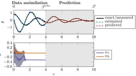
−0.5 0 0.5 0 0.2 0.4 0.6 0.8 1 b α(learned) α (original) b αNP+1 αNP+1 (a) 0 0.2 0.4 0.6 0.8 1 1 1.5 2 θ exact estimated predicted 0 0.2 0.4 0.6 0.8 1 −1 0 1 τ α b αNP+1
0Data assimilationTobs Prediction T
(b)
FIGURE 5Test Case 1. In (a), the colored circles represent the original parameters 𝛼𝑖plotted against the corresponding learned parameters ̂𝛼𝑖for the training individuals (𝑖 = 1, … , 𝑁
𝑃). Conversely, the black crosses represent the original parameters 𝛼𝑁𝑃+𝑘 plotted against the corresponding estimated parameters ̂𝛼𝑁𝑃+𝑘for the testing individuals. In the first row of (b) we show the
evolution of 𝜃𝑁𝑃+1(𝜏)(blue solid line), while the black dashed line represent the value of ̂𝜃𝑁𝑃+1(𝜏)estimated by means of the
EKF algorithm (for 𝜏 ∈ [0,Tobs]) and its predicted value (for 𝜏 ∈ (Tobs,T]). In the second row of (b), we show the evolution of the estimation of the value of ̂𝛼𝑁𝑃+1, with the ±3𝜎 bands, where 𝜎 denotes the standard deviation of the estimate.
between the two classes of parameters is easily detectable. Hence, we can conclude that the ANN-based model, learned from the data, is based on a different (but, possibly, equivalent) parametrization of the space of parameters.
In order to test the capabilities of the learned model to be used for classification and prediction purposes, we apply the procedure introduced in Sec. 2.1.3. Specifically, we consider a new individual, for which we randomly generate an initial state
𝜃𝑁𝑃+1
0 and a parameter 𝛼
𝑁𝑃+1. Similarly to what was done for the training individuals, we synthetically generate the evolution
of the state 𝜃𝑁𝑃+1(𝜏), for 𝜏 ∈ (0,T]by means of the original model (17). Then, we introduce an intermediate time instant
Tobs= 0.5 sand we imagine to observe the evolution of the new individual in the interval [0,Tobs]. In this time interval, we apply the EKF algorithm through the learned model ̂𝑔: more precisely, we solve Problem (8), in order to estimate the value of the parameter ̂𝛼𝑁𝑃+1 and of the state 𝜃𝑁𝑃+1(𝜏)(see Fig. 5(b)). We repeat the same protocol multiple times: we generate a
random initial state 𝜃𝑁𝑃+𝑘
0 and a random parameter 𝛼
𝑁𝑃+𝑘, for 𝑘 = 1, … , we generate the corresponding synthetic data, from
which, by means of DA, we estimate the values of ̂𝛼𝑁𝑃+𝑘. In Fig. 5(a), we plot the obtained pairs (̂𝛼𝑁𝑃+𝑘, 𝛼𝑁𝑃+𝑘). We notice
that the estimated values of ̂𝛼 are compliant with the one-to-one relationship between the parameters 𝛼 and the parameters ̂𝛼 that emerged in the training phase. Therefore, since in practical applications one cannot observe 𝛼𝑁𝑃+𝑘, while ̂𝛼𝑁𝑃+𝑘 can be
estimated, this provides a way of classifying the new individual. Indeed, the mere observation ̂𝛼𝑁𝑃+𝑘allows to conclude that the
(𝑁𝑃 + 𝑘)-th individual features characteristics similar to those of the individuals with a similar ̂𝛼.
As mentioned in Sec. 2.1.3, by exploiting the estimated value of ̂𝛼𝑁𝑃+1, the model ̂𝑔 can be exploited to predict the evolution
of 𝜃𝑁𝑃+1(𝜏)for 𝜏 ∈ (Tobs,T]. In Fig. 5(b) we report the prediction of 𝜃𝑁𝑃+1(𝜏)obtained by numerically approximating the
solution of Problem (10). We repeat the same protocol for 1000 synthetically generated testing individuals, obtaining an overall normalized 𝐿2error between the prediction and the exact solutions of 3.8 ⋅ 10−3.
In conclusion, even if the learned model does not coincide with the original one (it is indeed a trivial reformulation of it), thanks to the interplay between ML and DA, it can still be employed to classify individuals and to make predictions. In Sec. 2.3.4 we will deal with the problem of unequivocally selecting a unique representative model within a class of trivially reformulations of the same underlying model. However, before dealing with this topic, we show that something more subtle than a trivial reformulation may hinder the interpretability of the results.
−0.5 0 0.5 0 0.2 0.4 0.6 0.8 1 b α(learned) α (original) b αNP+1 αNP+1 (a) 0 0.2 0.4 0.6 0.8 1 1 1.5 2 2.5 3 θ exact estimated predicted 0 0.2 0.4 0.6 0.8 1 −1 0 1 τ α αb NP+1
0Data assimilationTobs Prediction T
(b)
FIGURE 6Test Case 2: (a) original parameters 𝛼𝑖plotted against the corresponding learned parameters ̂𝛼𝑖and (b) evolution of
𝜃𝑁𝑃+1(𝜏), of ̂𝜃𝑁𝑃+1(𝜏)and of the estimation of ̂𝛼𝑁𝑃+1. See caption of Fig. 5 for the notation.
2.3.2
Test Case 2: Non-trivial reformulations
Let us consider the following model, which we denote as Test Case 2, where the state is given by the two-dimensional vector
𝜃= (𝜃1, 𝜃2) ∈ ℝ2, while the parameter is one-dimensional ⎧ ⎪ ⎪ ⎨ ⎪ ⎪ ⎩ d d𝜏𝜃1(𝜏) = 𝛼 𝜃1(𝜏) 𝜏∈ (0,T], d d𝜏𝜃2(𝜏) = 0 𝜏∈ (0,T], 𝜃1(0) = 𝜃1,0, 𝜃2(0) = 𝜃2,0. (19) Test Case 2 is obtained from Test Case 1 by introducing a further state variable, with a trivial dynamics (𝜃2is clearly constant in 𝜏). However, even if the modification is only minimal, the results (shown in Fig. 6(a)) are significantly different from those obtained for the Test Case 1 (see Fig. 5(a)). Indeed, for Test Case 2 the parameters of the original model 𝑔 are not related with those of the learned one ̂𝑔 by a one-to-one relationship.
At first sight, we are tempted to conclude that the algorithm of Sec. 2.2 failed its goal of finding a good description of the training individuals. However, if we employ the learned model, as for Test Case 1, to predict the evolution of a new individual (by observing it over the time interval [0,Tobs], whereTobs= 0.5 s, and by estimating the parameter ̂𝛼𝑁𝑃+1through the EKF
algorithm), we still obtain good results (see Fig. 6(b)). As a matter of fact, by repeating the above mentioned protocol for 1000 synthetically generated individuals, we obtain an overall relative error of 3.7 ⋅ 10−3.
Since the obtained error is similar to that obtained for Test Case 1, we conclude that also for Test Case 2 the learned model is a faithful mathematical description of the original one. However, the model learned in Test Case 2 cannot be obtained from the original one simply by a change of variable in 𝛼. Hence, we say that model ̃𝑔 is a non-trivial reformulation of model 𝑔.
To provide an example that shows how a non-trivial reformulation of Model (19) can be obtained, we consider the following model ⎧ ⎪ ⎪ ⎨ ⎪ ⎪ ⎩ d d𝜏𝜃1(𝜏) = (̃𝛼+ 𝜃2(𝜏)) 𝜃1(𝜏) 𝜏∈ (0,T], d d𝜏𝜃2(𝜏) = 0 𝜏∈ (0,T], 𝜃1(0) = ̃𝜃1,0, 𝜃2(0) = ̃𝜃2,0. (20) If we set ̃𝛼(𝜔) = 𝛼(𝜔) − 𝜃2,0(𝜔), ̃𝜃1,0(𝜔) = 𝜃1,0(𝜔)and ̃𝜃2,0(𝜔) = 𝜃2,0(𝜔)for any 𝜔 ∈ Ω, then it follows that Models (19) and (20) generate the same data (i.e. 𝜃1(𝜏, 𝜔) = 𝜃1,0(𝜔)𝑒𝛼(𝜔)𝜏and 𝜃1(𝜏, 𝜔) = 0).
A less trivial example, where we do not have a constant state as in Model (19), is given by the following model ⎧ ⎪ ⎪ ⎨ ⎪ ⎪ ⎩ d d𝜏𝜃1(𝜏) = 𝛼 𝜃1(𝜏) 𝜏∈ (0,T], d d𝜏𝜃2(𝜏) = −𝛼 𝜃2(𝜏) 𝜏∈ (0,T], 𝜃1(0) = 𝜃1,0, 𝜃2(0) = 𝜃2,0. (21) A non-trivial reformulation of Model (21) is given by
⎧ ⎪ ⎪ ⎨ ⎪ ⎪ ⎩ d d𝜏𝜃1(𝜏) = (̃𝛼+ 𝜃1(𝜏)𝜃2(𝜏)) 𝜃1(𝜏) 𝜏∈ (0,T], d d𝜏𝜃2(𝜏) = −(̃𝛼+ 𝜃1(𝜏)𝜃2(𝜏)) 𝜃2(𝜏) 𝜏∈ (0,T], 𝜃1(0) = ̃𝜃1,0, 𝜃2(0) = ̃𝜃2,0, (22)
and by setting ̃𝛼(𝜔) = 𝛼(𝜔) − 𝜃1,0(𝜔)𝜃2,0(𝜔), ̃𝜃1,0(𝜔) = 𝜃1,0(𝜔)and ̃𝜃2,0(𝜔) = 𝜃2,0(𝜔)for any 𝜔 ∈ Ω. It easy to check that, due to the fact that the product 𝜃1(𝜏)𝜃2(𝜏)is constant in time, the two models produce the same data.
We notice that in both cases (Models (19) and (21)) there is a quantity 𝐶(𝜃) that is constant in time (we have 𝐶(𝜃) = 𝜃2and
𝐶(𝜃) = 𝜃1𝜃2, respectively). This quantity is a constant value characterizing individuals, as much as the parameters 𝛼: in both the above considered examples, indeed, the map between (𝛼, 𝐶(𝜃0))and (̃𝛼, 𝐶(̃𝜃0))is one-to-one. Conversely, in the formulations considered above, the constant 𝐶(𝜃) is embedded into the state, which could be reduced to a single variable. In other words, we are trying to model more than necessary: the state could be reduced to the first variable 𝜃1(𝜏), and the second variable 𝜃2(𝜏) can be obtained by solving 𝐶(𝜃(𝜏)) = 𝐶(𝜃0). For this reason, we say that a model that admits (respectively, does not admit) a non-trivial reformulation is non-minimal (respectively, minimal). In Sec. 2.3.3 we state rigorous definitions of these concepts.
To motivate the importance of model minimality, we recall that the parameter ̂𝛼𝑁𝑃+1estimated through a non-trivial
reformu-lation 𝑔 of a model ̂𝑔 is not related to the original parameter 𝛼𝑁𝑃+1by a one-to-one relationship. Hence, it cannot be employed
to infer knowledge on the 𝑁𝑃 + 1individual (classification purposes) and it hampers the intepretability of the learned model.
2.3.3
Definition of reformulation
In what follows, we identify a model written in the form of Eq. (14) with the triplet (𝑔, ,A). Moreover, we denote the solution map associated with such a model as 𝑠𝑔∶ ×A × [0, +∞) →, defined as 𝑠𝑔(𝜃0, 𝛼, 𝜏) = 𝜃(𝜏), where 𝜃(𝜏) is the solution of Eq. (14). We introduce the following definitions.
Definition 1. We say that a function ̃𝐴∶ ×A → ̃A is:
• trivial, if it is constant in its first argument; non-trivial, otherwise;
• non-pathological, if { ̃𝐴(𝜃0, 𝛼) ∶ 𝛼 ∈A} = ̃A for any 𝜃0∈; pathological, otherwise.
Definition 2. We say that (̃𝑔, , ̃A)is a reformulation of (𝑔, ,A)if there exists a non-pathological function ̃𝐴∶ ×A → ̃A
such that:
𝑔(𝑠𝑔(𝜃0, 𝛼, 𝜏), 𝛼) = ̃𝑔(𝑠𝑔(𝜃0, 𝛼, 𝜏), ̃𝐴(𝜃0, 𝛼)) ∀ 𝜃0∈, 𝛼 ∈A, 𝜏 ≥ 0. (23) Moreover, we say that (̃𝑔, , ̃A)is a
• non-trivial reformulation of (𝑔, ,A), if (23) holds for some non-trivial non-pathological function ̃𝐴;
• trivial reformulation if all the non-pathological functions ̃𝐴satisfying (23) are trivial.
Definition 3. A model (𝑔, ,A)is minimal if it does not admit any non-trivial reformulation.
We remark that the hypothesis that the function ̃𝐴be non-pathological is needed to avoid pathological situations, such as
the case when a reformulation if obtained by a mere piece-wise redefinition of the coefficient. Moreover, we remark that the definition of reformulation is motivated by the following result, for which the proof is given in A.
Proposition 1. Let (̃𝑔, , ̃A)be a reformulation of (𝑔, ,A)through the map ̃𝐴∶ ×A → ̃A. Then we have
We remark that minimality is an intrinsic property of models: it is not affected, for instance, by invertible transformations of either the inputs, the outputs or the parameters (such as scaling or nondimensionalization). Even if, as shown in Test Case 2, the methods proposed in this paper can be applied to any model (minimal and non-minimal ones), working with minimal models enhances the quantity of information that can be extracted from the learned model. This leads to the issue of devising tests to check minimality of models. Clearly, since the original model is not known in practical applications, the minimality of the model to be learned cannot in practice be analytically checked through the Def. 3. In the case that some a priori knowledge about the physical phenomenon is available, minimality could be deduced by means of physics-based considerations. The development of a posteriori numerical tests aimed at checking model minimality will be the subject of future works.
We recall an important concept, that is identifiability of models51,52.
Definition 4. Two parameters 𝛼1, 𝛼2∈A are said indistinguishable for the model (𝑔, ,A)if
∃ 𝜃0∈ ∀𝜏≥ 0 𝑠𝑔(𝜃0, 𝛼1, 𝜏) = 𝑠𝑔(𝜃0, 𝛼2, 𝜏). (25) Moreover, we define 𝐼(𝛼) = {𝛼∗s.t. 𝛼 and 𝛼∗are indistinguishable}.
Definition 5. We say that a model (𝑔, ,A)is identifiable if 𝐼(𝛼) = {𝛼} for any 𝛼 ∈A, that is
∀𝜃0∈, 𝛼1≠ 𝛼2∈A ∃𝜏∗>0 𝑠𝑔(𝜃0, 𝛼1, 𝜏∗)≠ 𝑠𝑔(𝜃0, 𝛼2, 𝜏∗) (26) In fact, if a model is identifiable, then the map from the parameter-trajectory map 𝛼 → {𝑠𝑔(𝜃0, 𝛼, 𝜏)}𝜏≥0is one-to-one, for each
𝜃0 ∈ . Conversely, if a model is not identifiable, then, for some choices of the initial condition 𝜃0 ∈ the DA assimilation problem of identifying the parameter 𝛼 from the trajectory {𝑠𝑔(𝜃0, 𝛼, 𝜏)}𝜏≥0is ill-posed. Hence, in this paper we assume that we work with identifiable models. We remark that for linear models identifiability can be assessed by standard criteria (e.g. by studying the spectral properties of the observability matrix43). Nonetheless, in this paper we consider the more general case of nonlinear parametric dynamical models.
2.3.4
Uniqueness of representation of models
Clearly, every model (even the minimal ones) admit trivial reformulations. Indeed, the parameter 𝛼 is never measured and so it is subject to changes of variables. This is linked to the black-box structure of the model learning Problem (P2). As a consequence, the solution of Problem (P2) is not unique. In order to transform such a problem into a problem with a unique solution, we need to select a representative model inside each class of trivial reformulations. In this section, we suggest a strategy to accomplish this goal. Specifically, we restrict the space of candidate models 𝑛by imposing some a priori constraints on the dependence of
𝑔on 𝛼.
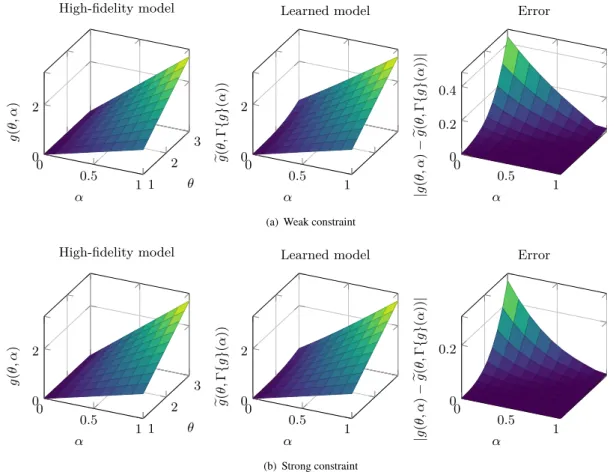
Let us suppose that there exists a function, Γ{𝑔(⋅, 𝛼)}(𝛼), expressed as a combination of 𝑔 and of its derivatives in 𝜃 (of any order) evaluated at some given points of , invertible in 𝛼. Then, we perform learning by restricting the search space to functions
𝑔 satisfying the constraint Γ{𝑔}(𝛼) = 𝛼. In what follows we will show that, in this way, the solution of the model learning
problem is unique.
This strategy can be interpreted as that of giving a physical meaning to the parameter 𝛼, which would be otherwise a black-box object. As a matter of fact, the constraint Γ{𝑔}(𝛼) = 𝛼 provides a definition of the parameter 𝛼. Let us consider the following example.
Example 1. Select some 𝜃∗ ∈ , and set Γ{𝑔}(𝛼) = 𝑔(𝜃∗, 𝛼). In this case, performing optimization under the constraint
𝑔(𝜃∗, 𝛼) = 𝛼is equivalent to defining the parameter as the time rate of change of the state at 𝜃∗.
The effectiveness of the proposed strategy is supported by the following proposition (the proof is given in A).
Proposition 2. Let (𝑔, ,A)be an identifiable model. Suppose that there exists an operator Γ{𝑔(⋅, 𝛼)}(𝛼), which acts on 𝑔 as a function of 𝜃, which is injective in 𝛼. Then, there exists a unique trivial reformulation of (𝑔, ,A)(that we denote by (̃𝑔, , ̃A)) such that Γ{̃𝑔}(̃𝛼) = ̃𝛼 for any ̃𝛼 ∈ ̃A.
From an implementative viewpoint, the constraint can be imposed in two alternative ways. The first (that we denote as weak
constraint) consists in adding to the loss function of Problem (P2) the following penalization term 𝑤2
2 ∫ A