Globis final report on Integrated Scenarios D30

(1)

HAL Id: hal-01300545

https://hal.archives-ouvertes.fr/hal-01300545

Submitted on 11 Apr 2016

HAL is a multi-disciplinary open access

archive for the deposit and dissemination of sci-entific research documents, whether they are pub-lished or not. The documents may come from teaching and research institutions in France or

L’archive ouverte pluridisciplinaire HAL, est destinée au dépôt et à la diffusion de documents scientifiques de niveau recherche, publiés ou non, émanant des établissements d’enseignement et de recherche français ou étrangers, des laboratoires

Globis final report on Integrated Scenarios D30

Florian Leblanc, C. Cassen, Thierry Brunelle, Patrice Dumas, Aurélie Méjean

To cite this version:

Florian Leblanc, C. Cassen, Thierry Brunelle, Patrice Dumas, Aurélie Méjean. Globis final report on Integrated Scenarios D30. [Research Report] Smash. 2014. �hal-01300545�

(2)

Globis final report on Integrated Scenarios D30

F. Leblanc, C. Cassen, T. Brunelle,P. Dumas, A.Mejean1

March 17, 2015

1_{Researchers at Centre International de Recherche sur l’Environnement et le}

D´eveloppement (CIRED,ParisTech/ENPC & CNRS/EHESS) - 45 bis avenue de la Belle Gabrielle 94736 Nogent sur Marne CEDEX, France. The authors wish to thankRuben Bibas

for his contributions on the energy/land-use coupling methodology within the Imaclim-R

(3)

Introduction

Since the Stockholm conference in 1972, the international community is seeking ways to better integrate development patterns and environmental issues. This is a huge challenge and an uneasy task given the complexity of underlying issues and geopolit-ical interests. The concept of sustainable development elaborated in the aftermath of the Brundtland report (United Nations World Commission on Environment and Development,1987) has been used as an inclusive narrative to take up the challenge. The European Union for instance has mainstreamed sustainable development in a broad range of its policies. Although regularly criticized for being too vague and not providing concrete solutions enough, this concept remains at the core of the agenda of international negotiations, in particular in the current process of Sustainable De-velopment Goals (SDGs)1_{. In parallel, the acceleration of the globalization process} over the last twenty years has been accompagnied by a redefinition of geopolitical balances. Most of economic sectors are impacted and new sources of tensions have emerged particularly on natural resources. A comprehensive approach that is able to encompass these multi-dimensional issues is then necessary to build sustainable development pathways.

The Globis project started by clarifying both concepts of sustainable develop-ment and globalization in WP1 and 2. The four case studies (energy/transport/landuse-food/ecoinnovation) elaborated in WP3 have shed lights on some key sustainability issues regarding the interactions between globalization and sustainable development, with a specific focus on long term trends. (Waisman et al.,2014) shows the sensi-tivity of long-term growth patterns at the global level and in an oil-importing and highly carbon emitting region like Europe2 to the features of long-term oil markets and to the implementation of climate policies. According to (Brunelle et al.,2014a), the production system may catch up with its biophysical asymptotes (in terms of

1

At the Rio+20 Conference in 2012 member States agreed to launch a process to develop a set of Sustainable Development Goals (SDGs), in view of the 2015 development agenda, see more information on http://sustainabledevelopment.un.org/?menu=1300

2

Indeed, given that imports supply 40% of European primary energy, corresponding to 2.8% of the EU GDP (Growth Domestic Product), energy security is a policy priority for the EU and its member states as put forward in recent official texts (see, e.g., the 2013 G&P)

(6)

availability of high quality lands) in case of subsequent shifts in food diets converging towards Western lifestyles while (K¨ohler et al., 2014) focuses on the conditions of the development of a second generation of biofuels in developing countries. (K¨ohler,

2014) envisages at least several pathways for green logistics and sustainable supply chain management to move toward sustainable transport (international shipping and long-haul aviation).

The final objective of the project is to provide an integrated vision of these four case studies in WP4. This deliverable will specifically analyze the conflicts and synergies between various sustainability issues that stem from these four cross sec-tors linkages under different visions of globalization and development pathways. The challenge is thus to integrate sector-based analysis in a common economic framework capturing the interplay between innovation, the evolution of life styles, macroeco-nomic constraints (investments, trade...) in a world experiencing strong ecomacroeco-nomic transitions.This report will then develop a set of comprehensive scenarios at the World and European levels. These numerical experiments will aim at analyzing i) the mechanisms that explain the tensions and synergies between various sustainabil-ity issues (climate change, land availabilsustainabil-ity, energy secursustainabil-ity) under various views of the future of economic globalization and ii) ways to mitigate these tensions within the framework of each scenario. We will specifically assess the implementation of cli-mate policies. CO2 emissions have indeed continued to grow in the past decade even more rapidly than predicted (Peters et al.,2011;Raupach et al.,2007;IPCC,2014). This context is the result of both the difficulty to decouple growth and carbon emis-sions in developed regions, where development styles cannot be changed overnight, and the rapid carbon-intensive growth patterns of emerging countries (IEA,2012). It also highlights the necessity to implement ambitious measures to trigger a strong bifurcation away from carbon-intensive development paths (IPCC,2007,2014)3. De-spite this scientific consensus, the implementation of ambitious global carbon emis-sion reduction targets remains highly uncertain as shown by the difficulties to reach a global climate agreement under the United Framework Convention on Climate Change (UNFCCC), in particular since the failure of the Copenhagen Conference in 2009. This is essentially due to the concerns about (a) significant welfare and economic losses consecutive to carbon restrictions and (b) the interplay of climate measures with other sensitive political issues such as the financial crisis, poverty al-leviation, job creation, energy and food security, or health and local environmental protection (e.g., see the dilemma of the climate development Gordian knot discussed in (Hourcade et al.,2008)). An integrated vision between sustainable development and the globalization process can be a precondition to overcome this dilemma in view of post 2015 climate policies.

To do that, we use the computable general equilibrium (CGE) model IMACLIM-R, which provides an innovative framework to organize the dialogue between

eco-3

At stabilization levels around 400 ppm CO2eq or below, global mean temperatures are likely to stay below 2°C, and there is a 50% probability of exceeding a 2°C temperature increase at levels of around 450 ppm CO2eq (IPCC,2007,2013)

(7)

nomics (to capture the general interdependences between sectors, issues and policy decisions), and engineering sciences (to capture the technical constraints and margins of freedom). It provides a multisectoral, dynamic modeling approach for thinking the link between growth, globalization, and energy constraints given the limited avail-ability of fossil resources and carbon mitigation policies. This framework captures four crucial determinants of the interplay between the energy sector, sustainability objectives, and globalization processes: (a) non marginal deviations with respect to current socioeconomic trends produce room for deep technical change over the course of the century 4 ; (b) beyond technological improvements, the integration of lifestyles, consumption patterns, and preferences in driving the material content of economic activity is captured (Mitchell, 2012); (c) limitations in the flexibility of technicoeconomic adjustments during transition processes affect the adaptability of the economy to sustainability constraints because of market imperfections, tech-nical inertias, and imperfect expectations; and (d) the competitiveness of opened economies on international markets impacts the balance of goods and capital. The IMACLIM modeling platform has been complemented by linking a specific module (the Nexus Land-Use model) to assess the feedbacks between land use dynamics and the rest of the economy.

Chapter2presents the set of storylines of the integrated scenarios and Chapter3 the rationale of the modeling approach. Chapter 4 quantifies the long term effect on the scenarios and highlights the main elements of discussions.

4_{Technical change is a change in the amount of output produced from the same inputs. Such a}

change is not necessarily technological but might include organizational transformations or be the result of a change in a constraint such as regulation, prices, or quantities of inputs.

(8)

Chapter 2

Definition of storylines

The first step of our methodology consists in building storylines which include the main features of the case studies. The challenge is to embark in a comprehensive manner detailed qualitative information in a quantitative/numerical model. To that end, we need to adapt the modeling platform but also include part of the qualitative information to inform relevant parameters. In this study, we build storylines around two main dimensions to integrate the four main issues of the project and we then assess the impact of a climate policy (see Fig.2.2).

The first dimension encompasses different features regarding development styles: energy consumption behaviors (that are directly linked to housing and people’s way/habit of consumption of goods) and the food diets (which directly impact agri-cultural practices and land use management). The second dimension captures the financial and trade aspects of the globalization process. Well-informed readers will see some similarities with the SRES scenarios (IPCC,2000) that assessed the main drivers of emissions, in particular the pursuit of the globalization process (although the SRES report considers only scenarios without climate policies)1. This work has not the ambitious to provide a new SRES exercise but tries to better understand the impact of some mechanisms of the globalization process related to trade and finance that were poorly considered in the SRES exercices.

For each dimension, we consider two extreme assumptions:

• Low intensive vs high intensive use of energy, transport and calory/meat in-tensive diets.

• Globalized vs regionalized trade (trade is gradually re-directed to regional markets) and capital markets.

By combining the two dimensions, we define four main scenarios representing four visions of development pathways:

1

Special Report on Emissions Scenarios. Published in 2000, the SRES scenarios cover a wide range of the main driving forces of future emissions, from demographic to technological and economic developments. Each scenario corresponds to one out four main storylines and was produced by modeling IIASA team (IPCC,2000)

(9)

Figure 2.1: Scenarios dimensions

• Scenario G1 (Glob HighCons) can be viewed as a benchmark case in the sense that it assumes a pursuit of current trends in energy consumption, food diets and international trade of goods and capital.

• Scenario G2 (Glob LowCons) describes a world wherein the globalization of trade and capitals continues but with a shift in terms of development path-ways, low energy consumption and a convergence toward sustainable feeding conditions (see section 3.2.1 for a detailed presentation of theses assumptions) • Scenario G3 (Frag HighCons) assumes a pursuit of current trends in energy consumption in a “fragmented” world. In this “fragmented” world, measures are undertaken to regulate the capital flows at the international scale in order to limit the risks of new financial crunch similar to 2008. Trade flows are also regulated at the international and regional level to protect local production in developing countries for harsh competition through feed in tariffs and also industrial productions in developed countries such as Europe.

• In Scenario G4 (Frag LowCons), the same shift in development pathways as observed in G2 senario occurs in a ”fragmented” world.

We then assess the impact of a climate policy. For the comparability of results, this article considers a unique climate objective. It consists of limiting the tem-perature increase with respect to preindustrial levels to +2.5°C, which is commonly believed to be more realistic than the +2°C 2_.

2_{The adoption of an ambitious global agreement on climate reduction emissions by 2015 and}

strong assumptions on technical change are indeed necessary to comply with the 2°C objective, which leaves little flexibility in terms of action (Edenhofer et al.,2010;Guivarch et al.,2011)

(10)

Figure 2.2: The four Scenarios

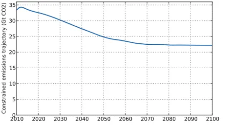
Following (Barker et al.,2007), this objective is translated into a carbon emission profile characterized by a peak of world CO2 emissions between 2010 and 2030 and a stabilization in 2050 with respect to 2000 levels (Fig.3.3).

(11)

Chapter 3

Methodology

The objective of this study is to integrate the energy, transport and land-use sectors in the same analytical framework. To cover these three sectors, we use two types of modelling tools: the IMACLIM-R model for the energy and transport sectors, and the Nexus Land-Use model for the land-use sector. This section describes the func-tioning of both models, as well as the methodology used for establishing a dialogue between these numerical tools.

3.1 IMACLIM-R

The risk of non-sustainable development stems ultimately from the joint effect of issues as diverse as climate change, energy and food security, land cover changes and social dualism in urban and rural areas. These issues in turn depend on the dynamics of consumption and technologies in sectors such as energy, transportation, construction and food production and on the hazards caused by shortages of pri-mary resources or by the transformation of our global environment. The challenge is thus to integrate sector-based analysis in a common economic framework capturing their interplay in a world experiencing very rapid demographic and economic transi-tions. The IMACLIM model was built in an attempt to address three methodological challenges through an integrated modelling approach (Weyant et al.,1996) to incor-porate knowledge from economics and engineering sciences, to support the dialogue with and between stakeholders and to produce scenarios with a strong consistency, concerning especially the interplay between development patterns, technology and growth. It adopts a dynamic, multiregion, and multisector representation of the world economy on the backbone1 _{of a CGE framework (see (}_{Waisman et al.}_,_2012a₎ for a detailed description). It provides a consistent vision of economic and energy

1_{The version of the IMACLIM-R model used in this study divides the world in 12 regions (the}

United States, Canada, Europe, Organisation for Economic Cooperation and Development [OECD] Pacific, former Soviet Union, China, India, Brazil, Middle East, Africa, rest of Asia, and rest of Latin America) and 12 sectors (coal, oil, gas, liquid fuels, electricity, air transport, water transport, other transport, construction, agriculture, energy-intensive industry, and services and light industry)

(12)

trajectories in yearly steps from 2010 to 2100 through the recursive succession of a top-down annual static equilibrium providing a snapshot of the economy at each yearly time step and through bottom-up dynamic modules informing the evolution of technical parameters between two equilibria (Fig. 3.1). The IMACLIM model is built as a platform which can include different modules depending on the issues tack-led. In this report, the IMACLIM model will be linked to the nexus land use which represents the agricultural and land use dynamics (see section 3.2 for a detailed description of the model).

Figure 3.1: Scenarios dimensions

The static equilibrium represents short-run macroeconomic interactions at each date t under technology and capacity constraints. It is calculated assuming Leontief production functions with fixed unitary intermediate consumption, labor inputs, and mark-up in non-energy sectors. Households maximize their utility through a trade-off between consumption goods, mobility services, and residential energy uses considering fixed end-use equipment. The equilibrium is given by market clearing conditions on all markets (including energy), which provides a snapshot of the econ-omy at date t in terms of relative prices, wages, employment, production levels, and trade flows.

The dynamic modules are reduced forms of bottom-up models, which describe the evolution of structural and technical parameters between t and t+1 in response to past and current economic signals. Each year, the regional capital accumulation is given by firms investment, households savings (controlled by exogenous saving rates like in (Solow,1956), and international capital flows. On that basis, the distribution

(13)

of investments across sectors is governed by expectations on sector profitability and technical conditions as described in sector-specific reduced forms of technology-rich models (see details in (Bibas et al.,2014) or in the supplementary material of ( Wais-man et al.,2012a)). These modules represent the evolution of technical coefficients resulting from agents’ microeconomic decisions on technological choices, given the limits imposed by the innovation possibility frontier (Ahmad, 1966). The new in-vestment choices and technical coefficients are then sent back to the static module in the form of updated production capacities and input output coefficients to calculate the equilibrium at t+1.

This modeling framework differs from conventional Integrated Assessment Mod-els (IAMs) by several features that make it relevant to study important specificities of sustainability transitions. First, the consistency of the iteration between the static equilibrium and dynamic modules relies on hybrid matrices, which ensure an explicit representation of the material and technical content of production processes through a description of the economy in consistent money values and physical quan-tities (Sands et al., 2005). Second, the equilibrium does not necessarily correspond to economic optimality because inertias on capital stocks limit the pace of technical change, the stickiness of the labor market affects labor adjustments, and market power leads to departures from marginal cost pricing. This means that production factors (production capacity and labor force) are not fully used, which ensures the possibility to represent idle capacities and unemployment. Third, contrary to the conventional assumption of intertemporally optimizing models, agents have imper-fect knowledge about the future and may make investment decisions according to biased expectations. This allows representing bifurcations, lockins, and potential cobenefits in the course of sustainable trajectories. Fourth, the hybrid structure of the model allows making explicit the technical assumptions behind the trajecto-ries, which can be informed by sector-based information and expert views about, for example, asymptotes on ultimate technical potentials, learning-by-doing mech-anisms, saturation in efficiency progress, the impact of incentive systems, and the role of market or institutional imperfections. Given the uncertainty on the long-term dynamics of these dimensions, their explicit representation allows considering variants of scenarios suited to capture alternative views on these controversial pa-rameters. Finally, contrary to the common approach of a unique composite good, the detailed multisectoral structure distinguishes productive sectors (agriculture, heavy industries, manufacturing, and services) according to their economic char-acteristics and their exposure to international trade. This allows a more precise description of the determinants of international trade. The next sections detail the modeling options adopted for the three core dimensions of the present study, de-velopment styles/consumption pathways, climate policy (Climate Constraints and Carbon Price), and international trade (Specifications for International Trade).

(14)

3.1.1 Modeling the Long-Term Dynamics of Oil Markets

Market mechanisms in the oil sector are driven by the utilization rate of production capacities, given by the ratio of total demand to production capacities: the higher the utilization rate, the higher the scarcity rent and the profit margin for oil producers (Robert K. Kaufmann and Sanchez,2004). We model the oil price formation through an explicit description of its geopolitical, technical, and economic determinants on both supply and demand. We represent (a) the heterogeneity of oil reserves as a function of their cost of production and conventional versus nonconventional nature; (b) the limitations on the short-term adaptability of oil supply due to the geological nature of reserves; (c) the market power of Middle East producers until the depletion affects the deployment of their production capacities; (d) technical change affecting the demand for liquid fuels in industry, residential, transport, and power sectors; and (e) the potentials and obstacles to the diffusion of biofuels and coal-to-liquid fuels as oil substitutes. These features of the representation of oil supply and demand dynamics are more extensively described in (Waisman et al.,2012b). In this report, we adopt median assumptions on the crucial determinants of oil price dynamics, namely the amount of reserves, geological inertias (assumed to be the same for conventional and nonconventional reserves), and the short-term price targeted by Middle East producers (assumed to be stabilized around its 2010 level).

3.1.2 Modeling development patterns

One of the scenario dimension concentrates on a few main drivers of development patterns, which are understood as constraints on behaviours and households’ pref-erences that impact energy consumption.

3.1.2.1 Private buildings

We introduce assumptions on the evolution of households’ preferences in housing. The ’Housing and Buildings’ module of Imaclim-R represents the dynamics of energy consumption as a function of the energy service level per housing square meter (heating, cooling, etc.) and the total housing surface. The former is represented by coefficients encompassing the technical characteristics of the existing stock of end-use equipment and buildings and the increase in demand for energy services: heating, cooking, hot water, lighting, air conditioning, refrigeration and freezing and electrical appliances. Housing surface per capita is driven by an income elasticity that drives the pace of convergence towards region-specific asymptotes of the floor area per capita.This limit reflects spatial constraints, cultural habits as well as assumptions about future development styles (including the lifestyles in emerging countries vis-` a-vis the US, European or Japanese way of life). For low consumption pathways (say G2 Glob LowCons and G4 Frag LowCons), a lower limit of the floor area per capita is taken for developing countries, as well as a lower income elasticity of building stock growth (including Former Soviet Union and Japan for constrasting scenarios). Finally, all scenarios include a household’s fuel price threshold that represents an

(15)

exit of fuel in private buildings heating. High Consumption pathways scenarios (G1 Glob HighCons and G3 Frag LowCons) stop using fuel in buldings from 1300$ within 20 years, while lower energy intensive scenarios (G2 Glob LowCons and G4 Frag LowCons) stop using fuel in buldings from 1000$ within 10 years.

3.1.2.2 Industrial goods consumption

Households’ industrial goods consumption are caped to consider a switch from in-dustrial goods to services as households gradually reach satiety in inin-dustrial goods equipment. The industrial and services sectors are each represented in an aggregated manner in the model, covering a large variety of economic sub-sectors and products. Technical change then encompasses not only changes and technical progress in each sub-sector but also the structural effects across sectors. In addition to autonomous energy efficiency gains, the Imaclim-R model represents the structural drop in energy intensity related to a progressive transition from energy-intensive heavy industries to manufacturing industries, and the choice of new techniques which results in both energy efficiency gains and changes in the energy mix. The progressive switch from industry to services is controlled by saturation levels of per capita consumption of industrial goods (in physical terms, not necessarily in value terms) via an asymp-tote calibrated as a possible multiplier of 2001 levels. For developing countries, these saturation levels represent various types of catch-up to the consumption style in developed countries. Saturation levels are supposed lower in low energy intensive scenarios (G2 Glob LowCons and G4 Frag LowCons).

3.1.2.3 Freight content of industrial production

In the freight sector, total energy demand is then driven by freight mobility needs, in turn depending on the level of economic activities and their freight content. Even though the share of transportation in total costs is currently low, decoupling freight mobility demand and economic growth is an important determinant of long-term mitigation costs. In the absence of such a decoupling (constant input-output coeffi-cient), and once efficiency potentials in freight transportation have been exhausted, constraining sectoral carbon emissions from freight transportation would amount to constraining economic activity. We thus build alternative evolutions of freight content of industrial good production (which includes both transport to the con-sumer as well as transport needs for inputs for the industrial production) through the transportation requirement per unit good produced. The later is slowly reduced in all regions for the constrained behavior scenarios (say G2 Glob LowCons and G4 Frag LowCons), hypothesis that are kept only for China and India otherwise (G1 Glob HighCons and G3 Frag HighCons).

3.1.3 Specifications for international trade of capital and goods

The endogenization of capital flows has hardly been integrated in global-scale energy-economy models because of a lack of shared empirical evidence and unresolved

(16)

con-troversies in the economic literature.2.

Following this diagnosis we adopt exogenous assumptions on the dynamics of capital flows, defined by the net balance between capital exports and imports, in-cluding the return to foreign direct investments. Base year imbalances on capital flows are explicitly represented through the calibration of capital imports/exports at the initial date. Their dynamics are ruled by two alternative assumptions:

• A constant over-time share of exported capital to model the persistence of current international capital imbalances

• An exponential decrease of all capital flows to represent a progressive decrease of international capital imbalances by 2050. This assumption corresponds to a vision of fragmented capital markets which imposes the financing of local investments by local capital.

All intermediate and final goods can be traded internationally, and total demand for each type of goods is met by a mix of domestic production and imports. Domestic and international markets for all goods are cleared (i.e. no stock is allowed) by a unique set of endogenous relative prices (the terms of trade), which adjust to maintain the equilibrium of the balance of payments defined by the sum of trade flows and capital flows. Trade flows are represented in physical quantities for energy flows (MToe), whereas all other goods are described with Armington specifications to capture imperfect substitutability among goods produced in different regions. We consider two parametric options to capture alternative visions of trade globalization: • A high value of Armington elasticities representing high substitutability be-tween goods produced in different places. This assumption favors current trends of international trade with intense competition and large import/export flows in all world regions.

• A low value of Armington elasticities representing low substitutability between goods produced in different places and a preference for local goods. This assumption comes down to envisage a slowing down of international trade and a re-regionalization of production close to demand.

3.2 Modelling the agricultural intensification and the

land constraint: The NLU model

3.2.1 General description of the NLU model

The Nexus Land-Use model (NLU) simulates changes in the agricultural sector at the global level under various assumptions regarding biomass demand (Souty et al.,

2012). The model relies on resource-use balance of crop and livestock products expressed in kilocalories (kcal), the common unit used for nutrition (1 kcal=4.1868

(17)

kJ). At the model base year (2001), the resource-use balance is established on the basis of data from the global database Agribiom (Dorin,2011). Using calories makes it possible to deal with different types of biomass for human consumption. In NLU, plant food, ruminant and monogastric calories are thus separated, and each type of calorie is associated with a specific production process.

Based on the livestock model provided by (Bouwman et al.,2005), monogastric animals are fed by a mix of food crops, residues and fodder. The production of ruminants is either intensive or extensive. In the intensive system, ruminants are fed by a mix of food crops, residues, fodder and grass, while they are exclusively fed with grass in the extensive system. In the NLU model, the frontier between the intensive and extensive systems evolve according to relative profits in each system. Crop- and pastureland for producing food crops and grass are endogenously modeled in NLU. On the other hand, the evolution of fodder area is mainly exogenously set (see infra).

The production of plant food calories (for food and feed use) is represented using a representative crop, as follows: at the base year, a representative potential yield is computed on a 0.5°×0.5° grid from the potential yields given by the vegetation model LPJmL for 11 crop functional types (CFT). Land classes grouping together grid points with the same potential crop yield are set up. Actual crop yield in each land class is determined by a non-linear function of chemical inputs, such as fertilisers and pesticides. In each land class, consumption of chemical inputs and associated crop yields are determined by cost minimisation. In this ways, NLU makes it possible to represent the land-fertiliser substitution by taking into account the land heterogeneity.

Two categories of crops are distinguished in NLU: “dynamic” crops, correspond-ing to most cereals, oilseeds, sugar beet and cassava, with a small share of fodder crops and “other” crops including sugar cane, palm oil, vegetables and fruits, some fodder crops and remaining crops. “Dynamic” crop yield is endogenously deter-mined, taking into account biophysical constraints and the amount of fertiliser used. The share of “other” crops in total crop production is supposed to be constant over the projection period 2005-2050. The “other” crop yield is an exogenous parameter calculated based on the projections from (Alexandratos and Bruinsma,2012).

In 2001 (model base year), the model is based on the land-use map from ( Ra-mankutty et al., 2008). The total cropland area amounts to 1472 Mha, divided between 748 Mha of “dynamic” crops and 724 Mha of “other” crops. Production on “dynamic” cropland represents ∼80% of the global calorie production reported by the global database Agribiom.

In NLU, three categories of pastures are distinguished. The two first are inten-sive and exteninten-sive pastures, corresponding to the two livestock production systems represented in NLU. A third category, called “residual”‘, is considered. This latter use of land is assumed to be inefficient in the sense that production cost is not min-imised. The residual pastures may correspond in reality to lands extensively man-aged because of geographic and institutional limitations (e.g. high transport cost, inadequate topography or specific land property rights). Residual pastures have the

(18)

same yield as extensive pastures. In the model base year, the total pasture area amounts to 2694 Mha following (Ramankutty et al., 2008). The quantification of total permanent pasture area is however highly uncertain due to the unclear distinc-tion between rangeland and grassland pastures in nadistinc-tional inventories (Ramankutty et al.,2008). In this study, we choose theRamankutty et al. (2008) dataset, which is believed to be more reliable than the FAO statistics, as the authors use a specific method relying both on satellite data and national inventories.

Two types of biomass for energy are represented in NLU: (i) first generation biofuel and (ii) short-rotation woody crops for bioelectricity (willow or poplar). Bioenergy production is modelled as a production constraint. Production of first generation biofuel is shared between biodiesel and ethanol based on the 2008 pro-duction (OECD and FAO,2008). The share of the different crops in 1st gen biofuel production is based on the 2006 production (Balat and Balat,2009;Brasil, Minist´erio da Agricultura, Pecu´aria e Abastecimento,2013). China and India are supposed to use only jatropha for biodiesel, not in competition with croplands. Biodiesel in Eu-ropean Union is produced from sunflower (5% ) and rapeseed (95%). Biodiesel in Africa and Rest of Asia is produced exclusively from palm oil.

The yield of feedstock for biofuel is set on the representative crop yield for the plant included in the “dynamic crop” (corn, wheat, sorghum, soybean, rapdeseed, sunflower). Palm oil plus kernel oil yield and palmkernel cake yield are taken from the last ten years. Sugarcane yield is taken from last ten years too. Cotton and Jatropha are supposed to represent a constant share of the other crop area.

By-products energy per ton of crop is computed by considering that the total energy per unit of mass in crop is available for byproducts, after oil, as well as transesterification (biodiesel) or fermentation (ethanol) losses are removed. The by-products energy content is substracted from the total calorie demand as long as it does not exceed the regional feed demand.

Yields of short-rotation woody crops is set on the gross annual increment (gai) provided by (Smeets et al., 2007, 39GJ/ha/year or 9.3Gcal/ha/year). The global gai value is scaled over the NLU regions according to the mean potential yield of our representative crop, assuming it is a reliable index of the land fertility. To account for the technological changes that may affect the woody biomass sector (in terms of harvest and species selection), we assume that the gai converge towards the net primary productivity reported by (Smeets et al.,2007, ∼120 GJ/ha or ∼30Gcal/ha) The performances of the model have been investigated through a backcasting exercise over the period 1961-2006. Estimations of cropland areas (sum of areas for “dynamic” and “other” crops) in each region are evaluated against historical data in each region from (Ramankutty and Foley,1999). At the global scale, the simulated cropland area fit observations rather well. The root-mean-square errors (RMSE) amounts to 52.3 Mha p.y. in absolute terms and 3.6% p.y. in relative ones.

(19)

3.2.2 Modeling development styles in NLU

The development styles/consumption pathways can be studied with NLU by test-ing two contrasttest-ing food demand scenario. The first one is the scenario produced in the 2012 revision of the foresight exercise from the Food and Agriculture Or-ganization if the United Nations (FAO) “World Agriculture Towards 2030/2050” (Alexandratos and Bruinsma, 2012). This scenario can be viewed as a business as usual pathway. According to their narrative, changes in diet will be a significant driver of the growth in the demand for agricultural products. However, convergence of diets towards developed countries should not completely level out consumption styles across developed and developing countries. In particular, substantial differ-ences may remain in the consumption of meat and milk. Regional food habits, such as taboos on cattle meat in India or pig meat in Muslim countries, will slow the “livestock revolution” experienced by countries like China, Brazil or Malaysia.

In contrast to this business as usual vision, we consider an alternative scenario based on a convergence towards sustainable feeding conditions, through (i) the re-duction in malnutrition and in the excesses in nutritional intake, (ii) the rere-duction in the share of animal calories in diets, and (iii) the reduction of food waste throughout the consumption process. This scenario is taken from the “Agrimonde 1” scenario of the French foresight exercise “Agrimonde” (Paillard et al.,2011b,a).

3.2.3 Specifications for international trade of agricultural goods

The international trade is modelled by using a pool representation without any consideration of the geographic origin of goods. Imports and exports are determined by relative regional calorie prices, taking into account a simple representation of imperfect competition and food sovereignty considerations. Coefficients governing the trade volume are calibrated against the year 2001 using Agribiom data. The (regional) price-elasticities of exports are calibrated against the 1961-2006 period.

For this exercise, the fragmentation of goods market are represented by reducing the value of the price-elasticity of trade reflecting the imperfect competition on the international markets of agricultural goods.

3.3 The coupling methodology IMACLIM-NLU

The objective of the coupling is to incorporate into the IMACLIM-R framework a representation of the land constraint which is consistent with biophysical potentials and farmer’s optimization behavior3. The coupling between IMACLIM and NLU is made in two steps. First, we implement a one-directional soft linking, in which IMACLIM feeds NLU with energy prices and a demand for bioenergy. Then, the hard coupling between the two models is implemented in a second step. We detail

3_{For a detailed description on bioenergy supply in IMACLIM-R, and its implications on CO} 2

(20)

in this report the whole coupling methodology, but the results will focus only on the first step.

3.3.1 One-directional soft linking

The energy prices (oil and gas price) computed by IMALCIM-R drives the fertiliser price used in NLU, and thus the level of intensification. At each timestep t, fertiliser price in NLU is computed at the world level based on an econometric relation with oil and gas price as follows:

log(P_f,tN LU) = α + β · log(P_f,t−1Obs ) + γ · log(PEner,t−1) + δ · log(PEner,t) (3.1)

With PEner=SN· Pgas+ (SP + SK) · Poil

SN, SP and SK correspond respectively to the share of N, P and K in the total NPK consumption. The index PEner, defined as the weighted sum of Pgas and Poil, is used to circumvent the colinearity issues between oil and gas prices. PObsf,t−1 refers to the observed fertilizer price values, and α, β, γ and δ denote the estimated parameters. More details are provided in (Brunelle et al.,2014b). The projection of the fertiliser price to 2100 is made based on the gas and oil price (secondary energy) coming from IMACLIM-R.

In this soft linking, IMACLIM computes the quantities of bioenergy (biofuel + woody biomass energy) that are necessary to reach a given emissions target, and send these quantites to NLU, which calculates the intensification level (mainly crop yield, share of extensive ruminant production and calorie price, as well as the corresponding CO2 and non CO2 emissions) to meet the demand for bioenergy.

3.3.2 Hard coupling

The basic functioning of the hard coupling between IMACLIM and NLU is described on Fig.3.2. To carry out this coupling, NLU has been modified to be driven by an exogenous price trend, rather than by a demand trend. The calorie price that equalizes the profitability of biofuel against the oil price (augmented by a carbon tax in the mitigation scenario) from IMACLIM-R is computed. NLU calculates the biofuel production which is economically profitable given this calorie price, and the other types of biomass that should be addressed.

The modelling of biomass for electricity relies on an different scheme. In this case, IMACLIM-R computes the quantities of biomass electricity that are economically profitable compared to other production options given the emissions target. These quantities are homogenously shared on the distribution of land used in the NLU model using the GAI as a proxy of the woody biomass yield (see section3.2).

To update the input-output coefficients in IMACLIM-R with the values com-puted in NLU, we need to disaggregate the agricultural sector of IMACLIM-R as it includes both the feedstock production sector (=agriculture, denoted “agri”) and the

(21)

(22)

food processing industry (=agroalimentary, not modelled in NLU, denoted “agro”). To do so, we use the GTAP database to split at the base year the hybrid matrix of the agricultural sector of IMACLIM into two subsectors, agri and agro. The agri sector is condsidered to be entirely determined by NLU, while the agro sector acts as a residue between the whole agricultural sector of IMACLIM-R and the agri sector. Thus, the coefficients of the agri sector are updated according to the evo-lutions computed in NLU, while the coefficients of the agro sector are deduced by substracting the updated coefficients of the agri sector from the coefficients of the whole agricultural sector computed by IMACLIM-R. Then the production and the profit margin of the agroalimentary subsector are deduced by considering a fixed share of labor and profit in the added value. In the same logic, the markup of the agricultural sector of IMACLIM-R evolves according to the land rent trajectories calculated by NLU.

A last step of the coupling consists in updating the intermediary coefficient of gas consumption in the industrial sector of IMACLIM-R to correctly account for the gas-intensive production process of fertilizers. To do so, we use the quantity of fertilizers used in agriculture provided by NLU, and we distinguish in the industrial sector of IMACLIM-R a subsector corresponding to the fertilizers production sector. The input-output coefficient of the two new sub-sectors (fertilizers production and other industrial sectors) are calibrated using the GTAP database.

3.3.3 Climate constraints and carbon price

Carbon emissions arising from the production and use of coal, oil, and gas are accounted for via coefficients capturing their respective carbon content.4_{. When} climate policies are implemented, a constraint on the profile of carbon emissions is imposed as a function of the chosen climate stabilization target (Fig. 3.3). This constraint on carbon emissions is satisfied thanks to the introduction of a market-based instrument in the form of a carbon price, which is considered by economists as the most efficient way to tackle the diversity of emissions of greenhouses gases and abatement sources in the economy (Aldy and Stavins, 2012). The carbon price increases the cost of final goods and intermediate consumption as a function of the carbon content of the energy used, and favors the adoption of carbon mitiga-tion opmitiga-tions in carbon-intensive sectors (industry, residential, power generamitiga-tion, and transport). After 2010, the carbon price value is endogenously calculated to abarte carbon emissions according to the prescribed objective, and associated revenues are collected (by the government) which are then reallocated to households or firms through transfers. A uniform climate policy in all regions and sectors and relying on a world-level carbon price instrument is obviously a simplification of what can be reasonably expected in the future, and is chosen for the sake of simplicity. It poses in particular a number of questions that are far beyond the scope of this report but are worth noting here: (a) monetary transfers to gain compliance of emerging

4

Those coefficients only account for actual emissions, and exclude carbon captured either bio-logically (biofuels) or technobio-logically (carbon capture and sequestration)

(23)

countries;10 (b) tax exemptions to protect certain specific activities (on the pattern of the EU-ETS for industrial activities); and (c) the role of accompanying measures to climate policies such as fiscal reforms, specific labor market policies (Guivarch et al.,2011), or complementary infrastructure policies (Waisman et al.,2013).

2010 2020 2030 2040 2050 2060 2070 2080 2090 21000 5 10 15 20 25 30 35

Constrained emissions trajectory (Gt CO2)

Climate constrained scenarios

(24)

Chapter 4

Results

4.1 IMACLIM-R standalone

4.1.1 Long-Term Oil Profiles and Macroeconomic Trajectories

In this section, we first consider the case where climate policy is not implemented, i.e. no constraint on carbon emissions is imposed. We study the dynamics of oil mar-kets and their macroeconomic effects on the transition toward low-oil development patterns as imposed by constraints on oil availability.

4.1.1.1 Dynamics of Oil Markets

In all scenarios, the world oil production follows an inverted U-shape reaching a max-imum around 2035-2040 (the so-called Peak Oil) before a continuous decrease over the long term, as shown in Figure4.2 for the bechmark scenario (Glob HighCons). Oil prices trajectories are characterized by three disctinct phases in the Benchmark scenario (Fig.4.1). Oil prices follow a slightly increasing plateau around 100 USD per barrel followed by a continuous increase at the date of Peak Oil (2040) to more than 500 USD per barrel in the long-term.

To analyze the effects of different asumptions regarding globalization and con-sumption pathways, we compare oil price trajectories in the G2, G3 and G4 scenarios with the trend in the G1 scenario (Glob HighEner) (Fig.4.3).

4.1.1.2 Globalization effect

In the short (between 2010 and 2040) and medium term (after 2040, i.e. during the Peak Oil period), oil prices are lower in globalized scenarios (G1 Glob HighEner and G2 Glob LowEner in Fig.4.3). This illustrates a moderation of the demand for oil. This is the result of higher capital availability that fosters technical change in a globalized context. Waisman et al. (2014) indeed show that less capital fluidity in a context of fragmented globalization slows down the pace of technical change towards more efficient technologies and triggers a higher dependence on oil. This in

(25)

2010 2020 2030 2040 2050 2060 2070 2080 2090 21000 100 200 300 400 500 600

World oil price $/ (Million b/d)

G1 (Glob_HighCons)

Figure 4.1: World oil price in$2001 / (Million b/d)

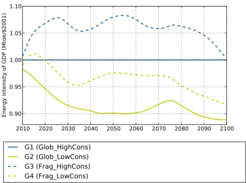
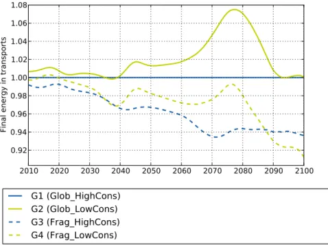
turn explains an increase of energy intensity of GDP after the peak oil (Fig. 4.4). In the long term, after 2080, however, energy intensity in G3 and 4 (Frag HighCons and Frag LowCons) tends to catch up with energy intensity in G1 (Glob HighCons) and G2 (Glob LowCons scenarios) scenarios. At that time, the economy is less dependent on international transport in the G3 and G4 scenarios, as shown by the lower energy content of transport, in particular for Europe in Figure4.5.

4.1.1.3 Consumption pathways effect

In the short term (between 2010 and 2040), assumptions behind low consumption pathways (G2 Glob LowCons and G4 Frag LowEner scenarios) favor a lower oil de-mand that results in lower oil prices as shown in Fig.4.3and lower energy intensity of GDP (Fig.4.4) compared to scenarios with business as usual development path-ways (G1 Glob HighCons and G3 Frag HighCons). This is the direct consequence of lower energy consumption in the residential sector, earlier saturation of consumers’ preferences for final goods and lower consumption of freight transport per unit of good produced (as described in chapter 2). During the Peak Oil period, lower con-sumption ascon-sumptions alleviate the impact of a lower technical change caused by less capital availability which result in higher energy intensity in Fragmented glob-alization scenarios.

(26)

2010 2020 2030 2040 2050 2060 2070 2080 2090 21000 20 40 60 80 100 120

World oil production (Million b/d)

G1 (Glob_HighCons)

Figure 4.2: World oil production (Million b/d)

We now study the consequences of the sustainability challenge posed by oil avail-ability on the stavail-ability of socioeconomic trajectories, as measured by the GDP trends. Differences in GDP among the four scenarios are relatively tenuous except in the G2 (Glob LowCons) scenario. However, when looking at different time periods, we observe more contrasted results. In the short and medium term (up to 2060), fragmented capital and good markets hurt the economy more significantly (scenar-ios G3 Frag HigCons and G4 Frag LowCons) than in globalized scenar(scenar-ios, whatever the assumptions regarding development styles. This is the result of the constraints these assumptions impose on both capital availability for investment in new tech-nologies and trade effects. Capital availability affects the resilience of the economy to rising oil prices, especially in oil importing economies such as Europe. A higher energy intensity of economic activity in a context of higher energy prices impacts households’ purchase power and firms’ production costs.The assumption on the re-gionalization of good markets has also crucial effects in driving the reaction of the European economy to the Peak Oil. In a context of high energy prices, the value of European energy imports significantly increases, resulting in a parallel increase of industrial exports to restore the equilibrium of the balance of payments. In a context of regionalized trade, which assumes preference for local goods, this can only occur through significant gains of competitiveness as measured by a decrease of the terms of trade and large real wage adjustments. Thus, these adjustments cause economic

(27)

2010 2020 2030 2040 2050 2060 2070 2080 2090 21000 500 1000 1500 2000 2500 3000 3500 4000 4500

World oil prices ($2001/Mtoe)

G1 (Glob_HighCons)

G2 (Glob_LowCons)

G3 (Frag_HighCons)

G4 (Frag_LowCons)

Figure 4.3: World oil price (normalized with benchmark G1)

losses as captured by 2030.

By contrast, at a longer horizon, the overall effect of the fragmentation is positive. The economy relies less on international trade, as local production mostly meets demand. This indeed entails lower oil demand and prices, which drives down energy dependency and production costs, and enhances household’s purchase power. This trend is strengthened in the case of low fossil energy consumption pathways (G4 Frag LowCons). Low energy consumption styles favor lower oil demand over the entire period and thus limit the impact of the Peak Oil, especially in a fragmented context (Table4.1) .

To conclude, assumptions on the nature of the globalization of capital and goods markets and behaviors impact the resilience of the economy faced with the oil con-straint. In particular, globalization impacts the pace of technical change and the dependence of the economy on international transport (in the long term), while the nature of development behaviors alleviate or strengthen the impact of the globaliza-tion assumpglobaliza-tions.

(28)

2010 2020 2030 2040 2050 2060 2070 2080 2090 2100 0.90 0.95 1.00 1.05 1.10

Energy intensity of GDP (Mtoe/$2001)

G1 (Glob_HighCons)

G2 (Glob_LowCons)

G3 (Frag_HighCons)

G4 (Frag_LowCons)

Figure 4.4: World energy intensity of GDP (normalized with benchmark G1)

4.1.2 The transition toward a low carbon society

4.1.2.1 Macroeconomic Effects of Climate Policies (World and Europe) The carbon price trajectory in Figure 4.6 displays three distinct phases. Between 2010 and 2030, the carbon price increases to reach 120$ per t/CO2 around 2030, with hardly any effect on oil prices that remain controlled by Middle East produc-ers. This carbon price level is necessary to tap most of mitigation potentials in the power, residential and industrial sectors, which represent the core of emissions reductions at that time (IPCC, 2007). Between 2030 and 2050, the carbon price decreases without hampering emissions reductions. Indeed, two mechanisms sustain the decarbonlization process: (i) the cost of low-carbon options decreases through learning by doing, and (ii) the oil price rise due to the Peak Oil although moderated further stimulates technical change in low carbon options, through the wider de-ployment of these technologies. After 2060, the increase in cabon prices is driven by the high cost of mitigation potentials in the transportation sector, which is weakly sensitive to energy prices.

(29)

2010 2020 2030 2040 2050 2060 2070 2080 2090 2100 0.92 0.94 0.96 0.98 1.00 1.02 1.04 1.06 1.08

Final energy in transports

G1 (Glob_HighCons)

G2 (Glob_LowCons)

G3 (Frag_HighCons)

G4 (Frag_LowCons)

(30)

2010 2020 2030 2040 2050 2060 2070 2080 2090 21000 50 100 150 200 250 300

Carbon tax ($2001/t CO2)

G1 (Glob_HighCons)

(31)

2010 2020 2030 2040 2050 2060 2070 2080 2090 21000 2000 4000 6000 8000 10000 12000

World coal production (Mtoe)

G1 (Glob_HighCons) G1 (Glob_HighCons_Clim) 2010 2020 2030 2040 2050 2060 2070 2080 2090 21000 1000 2000 3000 4000 5000 6000

World oil production (Mtoe)

G1 (Glob_HighCons) G1 (Glob_HighCons_Clim) 2010 2020 2030 2040 2050 2060 2070 2080 2090 21000 1000 2000 3000 4000 5000

World gas production (Mtoe)

G1 (Glob_HighCons) G1 (Glob_HighCons_Clim)

(32)

A climate policy significantly lowers the supply of oil, coal and gas (Figure4.7). More precisely, until 2030, the carbon price fosters lower oil and coal production, while gas demand increases as a substitute for oil and coal, due to lower carbon intensity of gas. Between 2030 and 2040, there is a return of coal (as a result of a decrease of the carbon price). After 2050, coal reaches a plateau (idem for gas). 4.1.2.2 Macroeconomic effects on Climate Policies on Europe

In Europe, on average, climate policies decrease the average growth rate from 1.37% to 1.28% for the benchmark scenario G1 (Glob HighCons) which is relatively mod-erate (0.01% losses on average per year) (Table4.2). Climate policies have however different macroeconomic effects depending on the time marker considered. In the short term (2010-2030), they slow down economic growth (from 2.03% to 1.76% per year). This is the result of the introduction of the carbon price, which impacts a carbon intensive European economy. In the medium term (between 2030 and 2050), climate policies trigger much faster economic growth (from 1.76% to 1.84% per year). This is a co-benefit of low carbon measures that foster a decreased oil dependency and lowers the effects of Peak Oil. This underlines the role of climate policies in preparing a sustainable future by hedging against the uncertainty on future oil sup-ply (Rozenberg et al.,2010). The picture changes in the long term, i.e. after 2050. Indeed, climate policies may then cause significant economic losses, due to the need to abate transport-related emissions, which requires a fast increase in carbon prices given the weak effect of price signals on this sector.

4.1.2.3 Impact of globalization and development styles

In the short to medium term, in Europe, GDP trends remain superior in a context of

globalization, whatever the assumptions on consumption pathways (G1 Glob HighCons Clim and G2 Glob LowCons Clim). Fragmented capital markets essentially undermine

growth until 2030 as shown in Table4.2. Indeed, this period requires fast technical change to start the decarbonization of the economy, which is hindered by the re-strictions on the availability of capital. By contrast, in the long term (after 2080), GDP is higher in fragmented scenarios (G3 + Clim Frag HighCons Clim and G4 + Clim Frag LowCons Clim) compared to globalized scenarios, as a result of a lower dependency to international transport.

Assumptions on consumption pathways tend to alleviate the impact of lower capital availability in the short term and after 2050. On the contrary, during the Peak Oil (between 2030 and 2050) scenario G4 + Clim (Frag LowCons Clim) shows a lower GDP growth rate compared to other scenarios. Indeed, low consumptions pathways limit the European industrial exports in order to offset the increase in Eu-ropean energy imports and thus restore the equilibrium of the balance of payments. A first conclusion from these results is that a carbon price may induce the risk of large economic downturns when the environmental constraints (depletion of fos-sil fuel resources and carbon constraint) force drastic but unanticipated economic

(33)

changes. For Europe, the cost of climate policies are also particularly dependent on the assumptions on globalization. Regarding capital flows, fragmented markets limit the access to capital and delay technical change. This affects the resilience of the economy to rising oil prices, especially in oil-importing economies such as Europe. This effect is persistent in the long term because of the cumulative effectss on technical change. This is partially counterbalanced by the reduction of trade volumes which has the advantage of reducing transport-related energy and carbon uses. Secondly, low energy pathways (as represented in the model) are insufficient to comply with the 2.5°C target and avoid transition costs in the short and long term, even in a globalized context.

4.2 One-directional soft linking

When NLU is forced by exogenous trajectories of bionergy demand (biofuel + woody biomass for electricity) and energy price from IMACLIM-R, the biophysical limits represented in the model (potential crop yield and land availability) are rapidly reached. In 2035, the model is not able to find a solution anymore.

As shown on Fig. 4.2, the demand for bioenergy coming from IMACLIM-R amounts to ∼50% of the total human demand for vegetal products in 2035, which has itself quite sharply risen since 2005. The bionergy demand is mainly composed of biofuel (¿95% in all scenario). This context of rapid growth in biomass demand triggers sizeable changes in the agricultural system. Between 2005 and 2035, the cropland area at the world scale expands by ∼+50% in all scenarios, reaching ∼2400 Mha in 2038. At the same time, the yield gap, defined as the gap between the po-tential yield and the actual yield divided by the gap between the popo-tential yield and the minimum yield, falls from 55% to 44% in the high food demand scenario and from 57% to 52% in the low food demand scenario.

In 2035, the bioenergy demand begins to rise sharply to reach ∼16 Pkcal (∼60 exajoules) in all scenarios in 2100, i.e. ∼200% of the total human demand for vegetal products. The rise in bioernegy demand is particularly strong in three regions : Latin America, USA, and Europe. In this scenario, Europe becomes the third biggest biofuel consumer in 2100, behind Latin America and USA.

Given the biophysical potential which is still available at this date, this rise in demand for biomass products requires an increase in crop yields and/or cropland which cannot be met by the NLU model, explaining why the model cannot find a solution beyond this date.

Biofuels in IMACLIM-R are represented using cost curves from (IEA, 2006). The penetration of biofuels on the liquid fuels market is based on these cost curves depending on their competitiveness and availability. Both aspects are calculated by equalling out the marginal production costs of each type of agrofuel and the price of fossil fuel, with an eventual increase due to a carbon tax in the case of climate policies.

(34)

Figure 4.8: Bioenergy demand from IMACLIM-R versus food demand to 2100

technological change and the maturation of so-called second-generation technologies: the cellulosic-lignite branch for ethanol and the biomass liquefaction branch for biodiesel. The land constraint is also taken into account but in a quite rough manner. In the NLU model, the land constraint is represent in much more detailed manner, with explicit links to actual biophysical data. In addition, the estimation of the land availability is consistent with the underlying scenarios in terms of demographic growth, per capita food consumption and deforestation.

The representation of the technological change is also different in NLU, as this model only considers technical options that are currently available. For this reason, 2nd generation bioful is not included in the study. Also, NLU does not consider any increase in potential yield due to modern varieties or improved agricultural practices. Thus, our results show that a detailed modelling of the land constraint is crucial for estimating the actual biofuel production. Also, the influence of technological change in the biofuel production sector appears to be determinant. In the NLU analytical framework, we see that the target of a 16 Petakcal (∼60 exajoules) bioen-ergy production in 2100 is not feasible given our scenarios on food consumption and forest areas.

Another data exchange between IMACLIM-R and NLU concerns the oil and gas price that are used to calculate the fertilizer price. The resulting index of nutrient price is displayed on Fig.4.2. In the climate scenarios, the fertiliser price are slightly lower than in the Baseline scenarios at the beginning of the simulation period, and

(35)

slightly higher at the end of it, mimicing the underlying evolution of the oil and gas prices. There is however little contrast among the different scenarios because of the relatively low value of the carbon price in the mitigation scenario (see section4.1). As a consequence, the influence of fertiliser price on farmer’s intensification is relatively homogenous among the different scenarios studied.

Figure 4.9: Fertiliser price index to 2100 in the 6 scenarios studied (base 100=2001).

4.3 A world without biofuel: Results from the

IMACLIM-R model

The one-directional soft linking between IMACLIM-R and NLU cast doubts upon the feasibility of large scale biofuel production. Another source of concerns about biofuel production relates to the emissions from indirect land-use changes (Searchinger et al., 2008, ILUC). Assuming that food demand is weakly elastic to price, any in-crease in the production of biomass fuel generates a rise of crop prices and creates an incentive to extend cultivated areas. From there, the ILUC concept refers to the displacement of crops (food and non-food) or pastures on uncultivated land, such as fallow or forest, resulting from the use of feedstock for agrofuels produc-tion, and generating emissions of organic carbon stored in the vegetation and the soils. Using the economic model FAPRI, and the life-cycle analysis model GREET, (Searchinger et al.,2008) estimated the ILUC emissions for an ethanol scenario in

(36)

the USA. Their results showed that, once ILUC emissions are taken into account, biofuel emits ∼50% more than the fossil fuel reference.

Following the study by (Searchinger et al.,2008), several evaluations have been made to confirm this diagnosis. Most of these studies converged towards a value of the ILUC emissions that puts into question the benefit of biofuel for mitigating climate change (De Cara et al.,2012).

Given these conclusions, we consider an extreme case wherein there is no devel-opment of biofuels, in particular for the G2 senario (Glob LowCons) which showed the strongest resilience among the others scenarios in the previous section. We then assess the impact on two indicators: energy intensity and GDP. In both sce-narios, energy intensity is lower when there is no biofuel after 2040 (at the time of the PO period). This is indeed the result in the baseline scenario of the ab-sence of other substitute than biofuel to oil all the more as oil prices are insufficient to foster the penetration CTL at that time. The economy is then constrained to use less energy. When a climate policy is applied, the moderation of the energy demand starts before 2040. In terms of macroeconomic impacts, less available en-ergy in the baseline without biofuels limits economic development and implies lower GDP growth. Lower GDP growth observed when a climate policy (compared to the scenario Glob LowCons Clim) is applied are also the result of the inertias of the transport sector after 2050.

Table 4.1: Europe mean GDP growth - baseline

2010-2100 2010-2040 2040-2080 2080-2100

G1 (Glob HighCons) 1.37% 2.08% 0.98% 1.1%

G2 (Glob LowCons) 1.43% 2.23% 0.96% 1.19%

G3 (Frag HighCons) 1.36% 1.95% 0.9% 1.39%

G4 (Frag LowCons) 1.39% 2.07% 0.86% 1.42%

Table 4.2: Europe mean GDP growth - climat

2010-2100 2010-2040 2040-2080 2080-2100

G1 (Glob HighCons Clim) 1.37% 2.08% 0.98% 1.1%

G2 (Glob LowCons Clim) 1.43% 2.23% 0.96% 1.19%

G3 (Frag HighCons Clim) 1.36% 1.95% 0.9% 1.39%

(37)

Chapter 5

Conclusion

This report is based on the view that the interplay between globalisation and sus-tainability should be studied within a comprehensive analytical framework that in-corporates two pivotal dimensions: market flexibility (for goods and capital) and changes in lifestyles and consumption pathways. Many social scientists consider the intensification of exchanges between countries as a strong driver for the standard-ization of people’s tastes and preferences through the spreading of Western lifestyles (Sklair,2002; Stephan et al., 2011). Thus, economic assessments of the impact of trade and capital openness on sustainable development require a consistent analysis of the changes in lifestyles and the subsequent evolution of consumption patterns.

To carry out this study, we developed an analytical framework that takes into account the market flexibility and different consumption patterns, using four sce-narios as inputs to the general equilibrium model IMACLIM-R and the land-use model NLU. Our results show that the transition to a low carbon economy is sig-nificantly affected by the globalization of capital and goods markets. Indeed, lower capital availability hinders technical change and the penetration of low energy and carbon technologies. On the contrary, a lower intensity of trade in a context of frag-mented globalization, by reducing the intensity of international freigth transport, limits the impacts of rising oil prices after the peak oil. Alternative consumption pathways can alleviate or worsen these impacts. Indeed, the globalization of capital and goods markets mainly determines the pace and the direction of the transition towards a low carbon economy. Consumption pathways influence the intensity of changes. For instance, assumptions on consumption pathways tend to alleviate the impact of lower capital availability. At a sectoral level, our findings reveal specifically the decisive role of transport dynamics. Indeed, the inertia of transport infrastruc-tures and logistic chains limits the transformation of this sector. Green logistics and sustainable supply-chain management, in part driven by the IT revolution, provide possible answers to this issue, as shown by (K¨ohler,2014) in the case of international shipping and long-haul aviation. Our scenarios also show that biofuels, as substi-tutes to oil in this sector, could have a significant impact on land-use dynamics. Linking the IMACLIM-R and NLU models reveals that the amount of biofuels

(38)

re-quired in all scenarios cannot be met because of land constraints. Indeed, restricted land availability and competition with food production, as well as the emissions related to indirect land-use changes, may hinder their development. Second genera-tion biofuels (from residues or crops growing on marginal land) may be an opgenera-tion to overcome these issues, but would require sustained eco-innovation efforts to become economically competitive with fossil fuels (see (K¨ohler et al., 2014) in particular for a detailed analysis of the economic and regulatory conditions for key developing countries).

From a research perspective, these findings show the importance of a detailed modeling of the land-use sector in integrated assessments of the globalization vs sustainability issue1. They also imply to pay a closer attention to the design of policies and their financing to support the transition towards a low oil and carbon society. In addition to the better integration of land use issues, these would be two major ways of improving our study. These are also main challenges on the scientific agenda of the wider Integrated Assessment Modeling community. First, by focusing only on the freight sector, our scenarios do not consider alternative assumptions on personal mobility, which is supposed to increase in the coming decades. The high costs entailed by the inertias of the transport sector could also be avoided by deploying infrastructures favoring sustainable cities, and low-transport production systems. Such infrastructure policies should be implemented early on (Waisman et al.,2013), which raises the crucial issue of their financing in the currently adverse context of high public debt. The IMACLIM model could yet be improved by ex-plicitly representing all determinants of capital allocation to analyze the conditions of an allocation of investments in accordance with sustainability objectives. ( Hour-cade and Shukla, 2013), building on (Hourcade et al., 2012), show the crucial role of organizing low-carbon finance that would be able to redirect capital funds to-wards low-carbon infrastructures. The redirection of investments still needs specific devices. For example, a social cost of carbon as part of a climate-friendly archi-tecture (possibly in a Post Kyoto framework) may enhance investors’ confidence in low-carbon projects and reduce the attractiveness of speculative investments.

From a perspective of sustainable development governance, this study has iden-tified possible tensions that relate to the combining process of globalization, con-sumption pathways and climate issues. These issues are to varying degrees on the agenda of multiple arenas of negotiations, such as the UNFCCC, the WTO (World Trade Organization) or the UN process of defining Sustainable Development Goals. Some see substantial progress of the internationalization of global challenges, others consider that the complex international architecture is unlikely to promote efficient issue-linkage among policies. This debate is beyond the scope of this report. We can simply conclude that one challenging issue for Europe is to try to make these agendas consistent by building a multi-level strategy in line with its own objectives: being a leader in the race of the upcoming so-called ”green industrial revolution”

1

For a model comparison of the importance of bioenergy supply modeling regarding long-run climate objectives, see (Rose et al.,2013).

(39)

in the fierce context of global competition, while allowing for inclusive development among all Member States. Given the internal political and social difficulties of the EU, this is without a doubt a daunting and exciting challenge of the coming years and decades.